On the Gibbs states of the noncritical Potts model on $\Z^{2}$

Abstract

We prove that all Gibbs states of the $q$-state nearest neighbor Potts model on $\mathbb{Z}^{2}$ below the critical temperature are convex combinations of the $q$ pure phases; in particular, they are all translation invariant. To achieve this goal, we consider such models in large finite boxes with arbitrary boundary condition, and prove that the center of the box lies deeply inside a pure phase with high probability. Our estimate of the finite-volume error term is of essentially optimal order, which stems from the Brownian scaling of fluctuating interfaces. The results hold at any supercritical value of the inverse temperature $\beta>\beta_{c}(q)=\log\left(1+\sqrt{q}\right)$.

Keywords: Potts model, Gibbs states, DLR equation, Aizenman-Higuchi theorem, translation invariance, interface flucutuations, pure phases
MSC2010: 60K35, 82B20, 82B24

1 Introduction

1.1 History of the problem

Since the seminal works of Dobrushin and Lanford-Ruelle [16, 29], the equilibrium states of a lattice model of statistical mechanics in the thermodynamic limit — the so-called Gibbs states — are identified with the probability measures $\mu$ that are solutions of the DLR equation,

$$\mu(\cdot)=\int\mathrm{d}\mu(\omega)\gamma_{\Lambda}(\cdot\,|\,\omega),\qquad\text{for all finite subsets $\Lambda$ of the lattice,}$$

where the probability kernel $\gamma_{\Lambda}$ is the Gibbsian specification associated to the system; see [19]. Under very weak assumptions (at least for bounded spins), it can be shown that the set $\mathcal{G}$ of all Gibbs states is a non-empty simplex. The analysis of $\mathcal{G}$ is thus reduced to determining its extremal elements. In general, this is a very hard problem which remains essentially completely open in dimensions $3$ and higher, for any nontrivial model, even in perturbative regimes.

The problem of determining all extremal Gibbs states amounts to understanding all possible local behaviors of the system. Pirogov-Sinaĭ’s theory [32, 35] often allows, at very low temperatures, to determine the pure phases of the model, i.e., the extremal, translation invariant (or periodic) Gibbs states, as perturbations of the corresponding ground states. However, it might be the case that suitable boundary conditions induce interfaces resulting in the local coexistence of different thermodynamic phases. That such a phenomenon can occur was first proved for the nearest-neighbor ferromagnetic (n.n.f.) Ising model on $\mathbb{Z}^{3}$ by Dobrushin [17], by considering the model in a cubic box with $+$ spins on the top half boundary of the box and $-$ spins on the bottom half (the so-called Dobrushin boundary condition). He proved that, at low enough temperatures, the induced interface is rigid — it is given by a plane with local defects — and the corresponding Gibbs state is extremal.

In two dimensions, the situation is very different. Gallavotti [18] proved, by studying the fluctuations of the corresponding interface, that the Gibbs state of the (very low temperature) n.n.f. Ising model on $\mathbb{Z}^{2}$ obtained using the Dobrushin boundary condition is the mixture $\tfrac{1}{2}(\mu^{+}+\mu^{-})$, where $\mu^{+}$ and $\mu^{-}$ are the two pure phases of the Ising model. This was refined by Higuchi [24], who proved that the interface, after diffusive scaling, weakly converges to a Brownian bridge at sufficiently low temperatures. These two results were then pushed to all subcritical temperatures by, respectively, Messager and Miracle-Sole [31] and Greenberg and Ioffe [22]. A weaker but very simple and general proof of the non-extremality of the state obtained using Dobrushin boundary condition can be found in [8].

The fact that the Dobrushin boundary condition gives rise to a translation invariant Gibbs state is a strong indication that all Gibbs states of the two-dimensional Ising model should be translation invariant: because of the large fluctuations of the interfaces, a small box deep inside the system should remain, with high probability, far away from any of the interfaces that are induced by the boundary condition. Thus the possible local behaviors of the system should correspond to the pure phases.

In the late 1970s, this phenomenology was established in the celebrated works of Aizenman [1] and Higuchi [25], based on important earlier work of Russo [34]. They proved that $\mathcal{G}=\{\alpha\mu^{+}+(1-\alpha)\mu^{-}\,:\,0\leq\alpha\leq 1\}$ for the n.n.f. Ising model on $\mathbb{Z}^{2}$. Their approaches relied on many specific properties of the Ising model (in particular, GKS, Lebowitz and FKG inequalities were used in the proof). A decade ago, Georgii and Higuchi [21] devised a variant of this proof with a number of advantages. In particular, their version only relies on the FKG inequality (and some lattice symmetries), which made it possible to obtain in the same way a complete description of Gibbs states in several other models: the n.n.f. Ising model on the triangular and hexagonal lattices, the antiferromagnetic Ising model in an homogeneous field and the hard-core lattice gas. It should be emphasized that all these works deal directly with the infinite-volume system, and have only very weak implications for large finite systems. In particular, the reasoning underlying these arguments (taking the form of a proof by contradiction) remains far from the heuristics of interfaces fluctuations.

A much more general result, restricted to very low temperatures, was established by Dobrushin and Shlosman [15]. They proved that, under suitable assumptions (finite single-spin space, bounded interactions, finite number of periodic ground states), all Gibbs states are periodic, and in particular are convex combinations of the pure phases corresponding to perturbations of the ground states of the model. Their approach deals with finite systems and is closer in spirit, if not fully in practice, to the above heuristics. Namely, even though interface fluctuations play a central role in the approach of [15], the authors resort to crude low temperature surgery estimates without developing a comprehensive fluctuation theory.

Very recently, a completely different approach to the Aizenman-Higuchi result was developed by two of us [13]. This new approach, although still restricted to the n.n.f. Ising model on $\mathbb{Z}^{2}$, presents several advantages on the former ones. Unlike [15] it does not require a very low temperature assumption, and actually holds for all sub-critical temperatures. Furthermore, it provides a quantitative, finite-volume version of the Aizenman-Higuchi theorem, with the correct rate of relaxation. Another interesting feature of the proof is that it closely follows the outlined heuristics and, consequently, should be much more robust.

In the present work, we extend the approach of [13] to n.n.f. Potts models on $\mathbb{Z}^{2}$. As will be seen below, two major factors make the proof substantially more difficult in this case. The first one is of a physical nature: In all previous non-perturbative studies, there were only two pure phases, and thus macroscopic interfaces were always line segments. In the Potts model with $3$ or more states, there are more than two phases and, consequently, interfaces are more complicated objects, elementary macroscopic interfaces being trees rather than lines. The second difficulty is of a technical nature: The positive association of Ising spins, manifested through the FKG inequality, simplified many parts of the proof in [13]. Unfortunately, this property does not hold anymore in the context of general $q$-state Potts models. We will therefore avoid this difficulty by reformulating the problem in terms of the random-cluster representation.

1.2 Statement of the results

Let $\Omega=\{1,\ldots,q\}^{\Z^{2}}$ be the space of configurations. Let $\Lambda$ be a finite subset of $\Z^{2}$, and $\Lambda^{c}=\Z^{2}\setminus\Lambda$ be its complement. The finite-volume Gibbs measure in $\Lambda$ for the $q$-state Potts model with boundary conditions $\sigma\in\Omega$ and at inverse-temperature $\beta>0$ is the probability measure on $\Omega$ (with the associated product $\sigma$-algebra) defined by

$$\mathbb{P}_{\beta,\Lambda}^{\sigma}(\eta)=\begin{cases}\frac{1}{Z^{\sigma}_{\beta,\Lambda}}{\rm e}^{-\beta H_{\Lambda}(\eta)}&\text{ if $\eta_{i}=\sigma_{i}$ for all $i\in\Lambda^{c}$}\\ 0&\text{ otherwise},\end{cases}$$

where the normalization constant $Z^{\sigma}_{\beta,\Lambda}$ is the partition function. The Hamiltonian in $\Lambda$ is given by

$$H_{\Lambda}(\eta)=-\sum_{\begin{subarray}{c}i\sim j\\ \{i,j\}\cap\Lambda\neq\varnothing\end{subarray}}\delta_{\eta_{i},\eta_{j}}$$

where $i\sim j$ if $i$ and $j$ are nearest neighbors in $\Z^{2}$. In the case of pure boundary condition $i\in\{1,\ldots,q\}$, meaning that $\sigma_{x}=i$ for every $x\in\Lambda^{c}$, we denote the measure by $\mathbb{P}_{\beta,\Lambda}^{(i)}$.

For an arbitrary subset $A$ of $\Z^{2}$, let $\mathcal{F}_{A}$ be the sigma-algebra generated by spins in $\Lambda$. A probability measure $\mathbb{P}$ on $\Omega$ is an infinite-volume Gibbs measure for the $q$-state Potts model at inverse temperature $\beta$ if and only if it satisfies the following DLR condition:

$$\mathbb{P}(\cdot|\mathcal{F}_{\Lambda^{c}})(\sigma)=\mathbb{P}^{\sigma}_{\beta,\Lambda}\qquad\text{ for $\mathbb{P}$-a.e. $\sigma$, and all finite subsets $\Lambda$ of $\mathbb{Z}^{2}$}.$$

Let $\mathcal{G}_{q,\beta}$ be the space of infinite-volume $q$-state Potts measures.

Non-emptiness of $\mathcal{G}_{q,\beta}$ can be proved constructively in this model. For $i\in\{1,\ldots,q\}$, ${(\mathbb{P}^{(i)}_{\beta,\Lambda})}_{\Lambda}$ converges when $\Lambda\nearrow\Z^{2}$ (in particular, the limit does not depend on the sequence of boxes chosen); this follows easily, e.g., from the random cluster representation. We denote by $\mathbb{P}^{(i)}_{\beta}$ the corresponding limit. It can be checked [20, Prop. 6.9] that the measures $\mathbb{P}^{(i)}_{\beta}$ ($i=1,\ldots,q$) belong to $\mathcal{G}_{q,\beta}$ and are translation invariant.

When $\beta$ is less than the critical inverse temperature $\beta_{c}(q)=\log(1+\sqrt{q})$ [6], it is known that there exists a unique infinite-volume Gibbs measure (in particular $\mathbb{P}^{(i)}_{\beta}=\mathbb{P}^{(j)}_{\beta}$ for every $i,j\in\{1,\ldots,q\}$). The relevant values of $\beta$ for a study of $\mathcal{G}_{\beta,q}$ are thus $\beta\geq\beta_{c}(q)$.

In the present work, we extend ideas of [13] in order to determine all infinite-volume Gibbs measures for the $q$-state Potts models at inverse temperature $\beta>\beta_{c}(q)$ on $\Z^{2}$. More precisely, we show that every Gibbs state is a convex combination of infinite-volume measures with pure boundary condition:

Theorem 1.1.

For any $q\geq 2$ and $\beta>\beta_{c}(q)$,

$$\mathcal{G}_{q,\beta}=\Bigl{\{}\sum_{i=1}^{q}\alpha_{i}\mathbb{P}_{\beta}^{(i)},\mbox{ where }\alpha_{i}\geq 0,\forall i\in\{1,\ldots,q\}\text{ and }\sum_{i=1}^{q}\alpha_{i}=1\Bigr{\}}.$$ (1)

A straightforward yet important corollary of this theorem is the fact that any Gibbs state is invariant under translations.

Corollary 1.2.

For any $q\geq 2$ and $\beta>\beta_{c}(q)$, all elements of $\mathcal{G}_{q,\beta}$ are invariant under translations.

A second important corollary is the fact that the extremal Gibbs measures (also called pure states) of the simplex $\mathcal{G}_{q,\beta}$ are the infinite-volume measures with pure boundary condition.

Corollary 1.3.

For any $q\geq 2$ and $\beta>\beta_{c}(q)$, the extremal elements of $\mathcal{G}_{q,\beta}$ are the $\mathbb{P}_{\beta}^{(i)},i\in\{1,\dots,q\}$.

This follows from Theorem 1.1: Define $\Delta(\beta)$ via $\mathbb{P}_{\beta}^{(i)}(\eta_{0}\neq i)=(q-1)\Delta$, and observe that in the decomposition (1) of $\mathbb{P}_{\beta}\in\mathcal{G}_{q,\beta}$, the coefficient $\alpha_{i}$ equals to $\frac{\mathbb{P}_{\beta}(\eta_{0}=i)-\Delta}{\mathbb{P}_{\beta}^{(i)}(\eta_{0}=i)-\Delta}.$

Actually, our main result is stronger than Theorem 1.1. As in [13], we obtain a finite-volume, quantitative version of the latter theorem, which, together with its proof, fully vindicates the heuristics given above. For a measure $\mu$ and an integrable function $f$, we write $\mu[f]=\int f\mathrm{d}\mu$.

Theorem 1.4.

Let $q\geq 2$ and $\beta>\beta_{c}(q)$, and set $\Lambda_{n}=\Z^{2}\cap[-n,n]^{2}$. For any $\varepsilon>0$ small enough, there exists $C_{\varepsilon}<\infty$ such that, for any boundary condition $\sigma$ on $\partial\Lambda_{n}$, we can find $\alpha_{1}^{n},\ldots,\alpha_{q}^{n}\geq 0$ depending on $(n,\sigma,\beta,q)$ only, such that

$$\bigl{|}\,\mathbb{P}_{\Lambda_{n},\beta}^{\sigma}[g]-\sum_{i=1}^{q}\alpha_{i}^{n}\,\mathbb{P}_{\beta}^{(i)}[g]\bigr{|}\leq C_{\varepsilon}\|g\|_{\infty}n^{-\tfrac{1}{2}+14\varepsilon},$$

for any measurable function $g$ of the spins in $\Lambda_{n^{\varepsilon}}$.

Note that the error term is essentially of the right order (which is $O(n^{-1/2})$); see [13] for a proof of this claim when $q=2$.

The strategy of the proof is the following. We consider the conditioned random-cluster measure on $\Lambda$ associated to the $q$-state Potts model with boundary condition $\sigma$. Boundary conditions for the Potts model get rephrased as absence of connections (in the random-cluster configuration) between specified parts of the boundary of $\Lambda$. In other words, boundary conditions for the Potts models correspond to conditioning on the existence of dual-clusters between some dual-sites on the boundary. Note that the conditioning can be very messy, since intricate boundary conditions correspond to microscopic conditioning on existence of dual-clusters. It will be seen that being a mixture of measures with pure boundary condition boils down to the fact that, with high probability, no dual-cluster connected to the boundary reaches a small box deep inside $\Lambda$ (which, in particular, implies that the same is true for the Potts interfaces).

The techniques involved in the proof are two-fold. First, we use positivity of surface tension in the regime $\beta>\beta_{c}$, which was proved in [6], in order to get rid of the microscopic mess due to the conditioning and to show that, deep inside the box, the conditioning with respect to $\sigma$ corresponds to the existence of macroscopic dual-clusters. The second part of the proof consists in proving that these clusters are very slim, and that they fluctuate in a diffusive way, so that the probability that they touch a small box centered at the origin is going to zero as the size of $\Lambda$ goes to infinity. The crucial step here is the use of the Ornstein-Zernike theory of sub-critical FK clusters developed in [10].

1.3 Open problems

Before delving into the proof, let us formulate some important open problems related to the present study.

$\blacktriangleright\;$Critical 2d Potts models. The behavior of two-dimensional $q$-state Potts models in the critical regime $\beta=\beta_{c}(q)$ is still widely open. It is conjectured that there is a unique Gibbs state when $q=3$ and $4$, but that, for $q\geq 5$, there is coexistence at $\beta_{c}$ of $q+1$ pure phases: the $q$ low-temperature ordered pure phases and the high temperature disordered phase. This is known to be true when $q$ is large enough [28, 30]. The extension of the latter result to every $q>4$ remains a mathematical challenge.

$\blacktriangleright\;$Finite-range 2d models. The extension of the present result, even in the Ising case $q=2$, to general finite-range interactions still seems out of reach today. There are, at least, two main difficulties when dealing with such models: On the one hand, it is difficult to find a suitable non-perturbative definition of interfaces (the classical definitions used, e.g., in Pirogov-Sinaĭ theory become meaningless once the temperature is not very low); on the other hand, interfaces will not partition the system into (random) subsystems with pure boundary conditions anymore, which implies that it will be necessary to understand relaxation to pure phases from impure boundary conditions. Of course, the general philosophy of the approach we use should still apply.

$\blacktriangleright\;$The question of quasiperiodicity. There is a general conjecture that two-dimensional models should always possess a finite number of extremal Gibbs states, all of which are periodic. In particular, this would imply that all Gibbs states are periodic, and thus that a two-dimensional quasicrystal cannot exist (as an equilibrium state).

$\blacktriangleright\;$Models in higher dimensions. Needless to say, the situation in higher dimensions is very different, due to the existence of translation non-invariant states. Even in the very low-temperature $3$-dimensional n.n.f. Ising model, the set of extremal Gibbs states is not known. Note, however, that it has been proved, in the case of a $d$-dimensional Ising model for any $d\geq 3$, that all translation invariant Gibbs states are convex combinations of the two pure phases at all temperatures [7]. A similar result also holds for large enough values of $q$ [30].

1.4 Notations

Each nearest-neighbor edge $e$ of $\Z^{2}$ intersects a unique dual edge of $(\Z^{2})^{*}=(\frac{1}{2},\frac{1}{2})+\Z^{2}$, that we denote by $e^{*}$. Consider a subgraph $G=(V,E)$ of $\Z^{2}$, with vertex set $V$ and edge set $E$. If $E$ is a set of direct edges, then its dual is defined by $E^{*}=\left\{e^{*}\,:\,e\in E\right\}$. Furthermore, if $G$ does not possess any isolated vertices, we can define the dual $V^{*}$ as the endpoints of edges in $E^{*}$. Altogether, this defines a dual graph $G^{*}=(V^{*},E^{*})$.

Let $\Lambda_{n}$ be the set of sites of $\Z^{2}\cap[-n,n]^{2}$ and $E_{n}$ be the set of all nearest-neighbor edges of $\Lambda_{n}$. The dual graph is denoted by $\left(\Lambda_{n}^{*},E_{n}^{*}\right)$. For $m<n$, the annulus $\Lambda_{n}\setminus\Lambda_{m}$ is denoted by $A_{m,n}$.

The vertex-boundary $\partial V$ of a graph $(V,E)$ is defined by $\partial V=\left\{x\in V:\exists y\sim x\ \text{such that $y\not\in V$}\right\}$.

The exterior vertex-boundary $\partial^{\rm ext}V$ of a graph $(V,E)$ is defined by $\partial^{\rm ext}V=\cup_{x\in V}\left\{y\not\in V:y\sim x\ \right\}$.

The edge-boundary $\partial E$ of a graph $(V,E)$ is the set of edges between two adjacent points of $\partial V$.

It will occasionally be convenient to think about $\partial E_{m}$ as a closed contour in $\mathbb{R}^{2}$ or, more generally, to think about subsets of $E$ (clusters, paths, etc) in terms of their embedding into $\mathbb{R}^{2}$; we shall do it without further comments in the sequel.

All constants in the sequel depend on $\beta$ and $q$ only. We shall use the notation $f=O(g)$ if there exists $C=C(\beta,q)>0$ such that $|f|\leq C|g|$. We shall write $f=\Theta(g)$ if both $f=O(g)$ and $g=O(f)$.

2 From Potts model to random-cluster model

In this section, we relate Potts and random-cluster models. We will assume throughout this article that the reader is familiar with the basic properties of the Fortuin-Kasteleyn (FK) representation. A very concise and clear exposition including derivation of comparison inequalities could be found in [2]. Mixing properties of random cluster measures were studied in [3, 4]. There is an extensive review [20] and a book [23] on the subject. More recent results [10, 6] play an important role in our approach.

Let $G=(V(G),E(G))$ be a finite graph. An element $\omega\in\{0,1\}^{E(G)}$ is called a configuration. An edge $e$ is said to be open in $\omega$ if $\omega(e)=1$ and closed if $\omega(e)=0$. We shall work with two types of boundary conditions: ${\sf f}$-free and ${\sf w}$-wired. Recall that the random-cluster measure with edge-weight $p$ and cluster-weight $q$ on $G$ with $*$-boundary condition ($*={\sf f},{\sf w}$) is given by

$$\mu_{G,p,q}^{*}(\omega)=\mu_{G}^{*}(\omega)=\frac{p^{\#\,\text{open edges}}(1-p)^{\#\,\text{closed edges}}q^{\#_{*}\,\text{clusters}}}{Z_{G,p,q}^{*}},$$

where $Z_{G,p,q}^{*}$ is a normalizing constant and a cluster is a maximal connected component of the graph $(V(G),\{e\in E(G)\,:\,\omega(e)=1\})$. The number $\#_{\sf f}\,\text{clusters}$ counts all the disjoint clusters, whereas the number $\#_{\sf w}\,\text{clusters}$ counts only those disjoint clusters which are not connected to the vertex boundary $\partial V$.

2.1 Coupling with a supercritical random-cluster model on $(\Z^{2})^{*}$

We consider the $q$-state Potts model on the graph $(\mathbb{Z}^{2})^{*}$ at inverse temperature $\beta>\beta_{c}(q)$. As the parameters $\beta$ and $q$ will always remain fixed, we drop them from the notation. Fix $\sigma\in\left\{1,\dots,q\right\}^{(\mathbb{Z}^{2})^{*}}$. For each $n$, we define the Potts measure $\mathbb{P}^{\sigma}_{\Lambda_{n}^{*}}$ on $\Lambda_{n}^{*}$ with boundary condition $\sigma$ on the vertex boundary $\partial\Lambda_{n}^{*}$.

It is a classical result (see, e.g., [2, 20]) that the Potts model can be coupled with a random-cluster configuration in the following way. From a configuration of spins $\eta\in\{1,\dots,q\}^{V(\Lambda_{n}^{*})}$, construct a percolation configuration $\omega^{*}\in\{0,1\}^{E_{n}^{*}}$ by setting each edge in $E_{n}^{*}$ to be

• closed if the two end-points have different spins,

• closed with probability ${\rm e}^{-\beta}$ and open otherwise if the two end-points have the same spins.

The measure thus obtained is a random-cluster measure on $(\Z^{2})^{*}$ with edge-weight $p^{*}=1-{\rm e}^{-\beta}$, cluster-weight $q$ and wired boundary condition on $\partial\Lambda_{n}^{*}$, conditioned on the following event, called ${\rm Cond}_{n}[\sigma]$: writing $S_{i}=\left\{x\in\partial\Lambda_{n}^{*}\,:\,\sigma(x)=i\right\}$, the sets $S_{i}$ and $S_{j}$ are not connected by open edges in $E_{n}^{*}$, for every $i\neq j$ in $\{1,\ldots,q\}$. We denote this measure by $\mu_{\Lambda_{n}^{*}}^{{\sf w}}(\cdot\;|\;{\rm Cond}_{n}[\sigma])$. When there is no conditioning, the random-cluster measure with wired (resp. free) boundary condition is denoted by $\mu_{\Lambda_{n}^{*}}^{{\sf w}}$ (resp. $\mu_{\Lambda_{n}^{*}}^{{\sf f}}$).

Reciprocally, the Potts measure can be obtained from $\mu_{\Lambda_{n}^{*}}^{{\sf w}}(\cdot\;|\;{\rm Cond}_{n}[\sigma])$ by assigning to every cluster a spin in $\{1,\ldots,q\}$ according to the following rule:

• For every $i\in\{1,\ldots,q\}$, sites connected to $S_{i}$ receive the spin $i$,

• The sites of a cluster which is not connected to $S_{i}$ receive the same spin in $\{1,\ldots,q\}$ chosen uniformly at random, independently of the spins of the other clusters.

Thanks to the connection between Potts measures and random-cluster measures, tools provided by the theory of random-cluster models can be used in this context. Note that the parameters of the corresponding random-cluster measure are supercritical ($p^{*}>p_{c}(q)$).

2.2 Coupling with the subcritical Random-Cluster model on $\Z^{2}$

Rather than working with the supercritical random-cluster measure on $(\Z^{2})^{*}$, we will be working with its subcritical dual measure on $\Z^{2}$ (this is the reason for choosing to define the Potts model on $(\Z^{2})^{*}$). There is a natural one-to-one mapping between $\left\{0,1\right\}^{E_{n}^{*}}$ and $\left\{0,1\right\}^{E_{n}}$. Namely, set $\omega(e)=1-\omega(e^{*})$. In this way, both direct and dual FK configurations are defined on the same probability space. In the sequel, the same notation will be used for percolation events in direct and dual configurations. For instance, $\omega\in{\rm Cond}_{n}[\sigma]$ means that $\omega^{*}\in{\rm Cond}_{n}[\sigma]$. The corresponding direct FK measure is $\mu^{{\sf f}}_{\Lambda_{n}}(\cdot\;|\;{\rm Cond}_{n}[\sigma])$.

It is well-known [11] that this defines an FK measure with parameters $q$ and $p$ satisfying $pp^{*}/[(1-p)(1-p^{*})]=q$.

Since we are working with the low temperature Potts model, the random-cluster model on $(\Z^{2})^{*}$ corresponds to $p^{*}>p_{c}(q)$ so that the random-cluster model on $\Z^{2}$ is subcritical ($p<p_{c}(q))$. For this measure, ${\rm Cond}_{n}[\sigma]$ is an increasing event which requires the existence of direct open paths disconnecting different dual $S_{i}$-s. This reduces the problem to the study of the stochastic geometry of subcritical clusters. In particular, this enables us to use known results on the subcritical model.

Let us recall the few properties we will be using in the next sections. First, there is a unique infinite-volume measure, denoted $\mu_{\mathbb{Z}^{2}}$. Second, there is exponential decay of connectivities in the random-cluster model with parameter $p<p_{c}(q)$. These two properties imply the following corollary.

Proposition 2.1.

There exists $c>0$ such that, for $n$ large enough and $2k\leq n\leq m$,

$$\mu_{A_{k,n}}^{\sf w}(\text{there exists a crossing of $A_{k,n}$})\leq{\rm e}^{-cn},$$

$$\mu_{\Lambda_{n}}^{\sf w}(\text{there exists a cluster of cardinality }m\text{ in }\Lambda_{n/2})\leq{\rm e}^{-cm},$$

where a crossing is a cluster of $A_{m,n}$ connecting the inner box to the outer box.

A cluster surrounding the inner box of $A_{m,n}$ inside the outer box of $A_{m,n}$ is said to be a circuit. Note that the existence of a dual circuit is a complementary event to the existence of a crossing between the inner and outer boxes.

Proposition 2.1 follows from the exponential decay of connectivities proved for any $p<p_{c}(q)$ in [6] together with the uniqueness of the infinite-volume measure (this is required to tackle wired boundary conditions, see [10, Appendix] for details). The result would not be true at criticality when $q$ is very large, despite the fact that there is exponential decay for free boundary conditions.

Surface tension

Surface tension in the supercritical dual model is the inverse correlation length in the primal sub-critical FK percolation. Let $p<p_{c}(q)$. The surface tension in direction $x$ is defined by

$$\tau(x)=\tau_{p}(x)=-\lim_{k\to\infty}\frac{1}{k}\log\mu_{\Z^{2}}(0\leftrightarrow[kx]),$$

where $y\leftrightarrow z$ means that $y$ and $z$ belong to the same connected component. We will also refer to it as the $\tau$-distance. By Proposition 2.1, $\tau$ is equivalent to the usual Euclidean distance on $\mathbb{R}^{d}$. Furthermore, by [10] it is strictly convex, and the following sharp triangle inequality of [26, 33] holds: There exists $\rho=\rho(p)>0$ such that

$$\tau(x)+\tau(y)-\tau(x+y)\geq\rho(|x|+|y|-|x+y|).$$ (2)

Define ${\rm d}_{\tau}(A,B)=\sup_{a\in A}\inf_{b\in B}\tau(a-b)$ to be the $\tau$-Hausdorff distance between two sets.

2.3 Reformulation of the problem in terms of the subcritical random-cluster model

Theorem 2.2.

Fix $p<p_{c}(q)$ and let $\varepsilon\in(0,1)$. Then, uniformly in all boundary conditions $\sigma$,

$$\mu_{\Lambda_{n}}^{\sf f}\bigl{(}{\mathsf{C}}\cap\Lambda_{n^{\varepsilon}}\neq\varnothing\;|\;{\rm Cond}_{n}[\sigma]\bigr{)}=O(n^{-\frac{1}{2}+14\varepsilon})$$ (3)

where $\mathsf{C}$ is the set of sites connected to the boundary $\partial\Lambda_{n}$.

The proof of this theorem will be the core of the paper. Before delving into the proof, let us show how it implies Theorem 1.4.

Lemma 2.3.

Let $\beta>\beta_{c}(q)$. Then,

$$\mathbb{P}^{\sf f}_{(\mathbb{Z}^{2})^{*}}=\frac{1}{q}\sum_{i=1}^{q}\mathbb{P}^{(i)}_{(\mathbb{Z}^{2})^{*}}.$$ (4)

Proof.

Fix $\beta>\beta_{c}$. Note that $\mathbb{P}^{(i)}_{(\mathbb{Z}^{2})^{*}}$ can be defined via the coupling with the random-cluster measure as follows. Let $\mu_{(\mathbb{Z}^{2})^{*}}$ be the unique infinite-volume random-cluster measure on $(\mathbb{Z}^{2})^{*}$. Since $p^{*}>p_{c}(q)$, this measure possesses a unique infinite cluster. The Potts measure $\mathbb{P}^{(i)}_{(\mathbb{Z}^{2})^{*}}$ is constructed by assigning spin $i$ to the infinite cluster, and a spin chosen uniformly at random for each finite cluster, independently of the spin of the other clusters. The Potts measure $\mathbb{P}^{\sf f}_{(\mathbb{Z}^{2})^{*}}$ can also be constructed from $\mu_{(\mathbb{Z}^{2})^{*}}$ by assigning to each cluster (including the infinite one) a spin chosen uniformly at random, independently of the spin of the other clusters. We deduce (4) immediately.

Note that in general, $\mathbb{P}^{(i)}_{(\mathbb{Z}^{2})^{*}}$ is constructed from the infinite-volume random-cluster measure $\mu_{(\Z^{2})^{*}}^{{\sf w}}$ while $\mathbb{P}^{\sf f}_{(\mathbb{Z}^{2})^{*}}$ is constructed from the infinite-volume random-cluster measure $\mu_{(\Z^{2})^{*}}^{{\sf f}}$. Therefore, if these two measures are different, (4) will not be valid. This is the case when $p=p_{c}(q)$ and $q$ is large enough. ∎

Lemma 2.4.

There exists $c>0$ such that, for any $n>0$ and any subdomain $\Omega^{*}$ of $(\Z^{2})^{*}$ containing $\Lambda_{2n}^{*}$,

$$\mathbb{P}^{\sf f}_{\Omega^{*}}[g]=\mathbb{P}^{\sf f}_{(\Z^{2})^{*}}[g]+O(\|g\|_{\infty}{\rm e}^{-cn}),$$ (5)

for any $g$ depending only on spins in $\Lambda_{n}^{*}$. The same holds for pure boundary conditions $i\in\{1,\ldots,q\}$.

Proof.

We treat the case of the free boundary condition. The other cases follow from the same proof. Since $p<p_{c}(q)$, the random-cluster model on $\Z^{2}$ has exponential decay of connectivities. Therefore, [4, Theorem 1.7(ii)] implies the so-called ratio strong mixing property for the dual random-cluster model: If a percolation event $A$ depends on edges from $E_{A}$ and if $B$ depends on edges from $E_{B}$, then,

$$\left|\frac{\mu^{{\sf f}}_{(\mathbb{Z}^{2})^{*}}(A\cap B)}{\mu^{{\sf f}}_{(\mathbb{Z}^{2})^{*}}(A)\mu^{{\sf f}}_{(\mathbb{Z}^{2})^{*}}(B)}-1\right|\leq\sum_{e_{A}\in E_{A},e_{B}\in E_{B}}{\rm e}^{-c\,{\rm d}(e_{A},e_{B})},$$ (6)

where ${\rm d}(e_{A},e_{B})$ is a distance between edges $e_{A}$ and $e_{B}$ (for instance the distance between their mid-points).

Together with the observation that $\mu^{{\sf f}}_{\Omega^{*}}=\mu_{(\Z^{2})^{*}}^{{\sf f}}(\cdot|\omega(e)=0,\forall e\notin E(\Omega^{*}))$, this leads to

$$\bigl{\lvert}\mu^{{\sf f}}_{\Omega^{*}}[f]-\mu_{(\Z^{2})^{*}}^{{\sf f}}[f]\bigr{\rvert}=O\bigl{(}{\rm e}^{-cn}\mu_{(\Z^{2})^{*}}^{{\sf f}}[f]\bigr{)}$$ (7)

for any function $f$ depending only on edges in $E_{3n/2}^{*}$. More generally, let $F$ be the event that there does not exist an open crossing in the annulus $A_{n,3n/2}$ (this corresponds to the existence of a dual circuit surrounding the origin). The complement $F^{c}$ of this event has exponentially small probability by Proposition 2.1. Consider a function $f$ depending a priori on every dual edges, but with the property that $f\mathbf{1}_{F}$ is measurable with respect to edges in $E_{3n/2}^{*}$. We immediately find that

$$\mu^{{\sf f}}_{\Omega^{*}}[f]=\mu^{{\sf f}}_{\Omega^{*}}[f\mathbf{1}_{F}]+O\big{(}||f||_{\infty}\mu^{{\sf f}}_{\Omega^{*}}(F^{c})\big{)}=\mu^{{\sf f}}_{\Omega^{*}}[f\mathbf{1}_{F}]+O(||f||_{\infty}{\rm e}^{-cn})$$

and similarly for $\mu^{\sf f}_{(\Z^{2})^{*}}[f]$, so that (7) is preserved for this class of functions.

Now, consider $g$ depending only on spins in $\Lambda_{n}^{*}$. Via the coupling with the random-cluster model, $\mathbb{P}^{\sf f}_{\Omega^{*}}[g]$ and $\mathbb{P}^{\sf f}_{(\Z^{2})^{*}}[g]$ can be seen as $\mu^{{\sf f}}_{\Omega^{*}}[f]$ and $\mu^{{\sf f}}_{(\Z^{2})^{*}}[f]$ for a certain function $f$, depending a priori on every edge, but for which $f\mathbf{1}_{F}$ depends on edges in $E_{3n/2}^{*}$ only (on the event $F$, the dual connections between vertices of $\Lambda_{n}^{*}$ are determined by edges in $E_{3n/2}^{*}$). We conclude that

$$\big{|}\mathbb{P}^{\sf f}_{\Omega^{*}}[g]-\mathbb{P}^{\sf f}_{(\Z^{2})^{*}}[g]\big{|}=\big{|}\mu^{{\sf f}}_{\Omega^{*}}[f]-\mu^{{\sf f}}_{(\Z^{2})^{*}}[f]\big{|}=O\big{(}||f||_{\infty}{\rm e}^{-cn}\big{)}.$$

∎

Figure 1: On the left (resp. center, right), the event $\mathcal{E}$ (resp. $\mathcal{F}^{\sf f}$, $\mathcal{F}^{(i)}$) is depicted.

Proof of Theorem 1.4.

Fix $n>0$ and a boundary condition $\sigma$ on $\partial\Lambda_{n}$. Fix $\varepsilon>0$ small.

We consider the coupling $(\eta,\omega)$ (the measure is denoted by $\mathbf{P}$) with marginals $\mathbb{P}^{\sigma}_{\Lambda_{n}}$ and $\mu^{\sf f}_{\Lambda_{n}}(\cdot\;|\;{\rm Cond}_{n}[\sigma])$ described in the previous section. Let $\mathcal{E}$ be the event that $\omega$ contains an open crossing in $A_{2n^{\varepsilon},n}$. Let $\mathcal{F}^{\sf f}$ be the event that $\omega$ contains an open circuit in $A_{2n^{\varepsilon},n}$. Let $\mathcal{F}^{(i)}$ be the event that $\omega$ contains neither an open crossing nor an open circuit in $A_{2n^{\varepsilon},n}$, and that $(\Lambda_{2n^{\varepsilon}})^{*}$ is connected in the dual configuration to $S_{i}$. Note that

$$\mathbf{P}(\mathcal{E})=\mu^{\sf f}_{\Lambda_{n}}(\mathcal{E}\;|\;{\rm Cond}_{n}[\sigma])=O(n^{-\frac{1}{2}+14\varepsilon}),$$

by applying Theorem 2.2.

• (conditioning on $\mathcal{F}^{\sf f}$). Let $\Gamma^{*}$ be the connected component of $\partial\Lambda_{n}^{*}$ in $\omega^{*}$. Denote the connected component of $\Lambda_{2n^{\varepsilon}}^{*}$ in $\Lambda_{n}^{*}\setminus\Gamma^{*}$ by $\Omega^{*}$. We have $\Lambda_{2n^{\varepsilon}}^{*}\subset\Omega^{*}$. Conditioning on $\Gamma^{*}$ we infer, using (5) and (4) that

  $$\mathbf{P}\bigl{(}g\bigm{|}\mathcal{F}^{\sf f}\bigr{)} =\mathbf{P}\bigl{(}\mathbb{P}^{\sf f}_{\Omega^{*}}[g]\bigm{|}{\mathcal{F}}^{\sf f}\bigr{)}=\mathbb{P}^{\sf f}_{(\Z^{2})^{*}}[g]+O(\|g\|_{\infty}{\rm e}^{-cn^{\varepsilon}})$$

  $$=\frac{1}{q}\sum_{i=1}^{q}\mathbb{P}^{(i)}_{(\Z^{2})^{*}}[g]+O(\|g\|_{\infty}{\rm e}^{-cn^{\varepsilon}}).$$

• (conditioning on $\mathcal{F}^{(i)}$). In this case, let us condition on the connected cluster $\Gamma$ of $\partial\Lambda_{n}$. We view $\Gamma$ as the set of bonds. Define $\Omega^{*}$ as the connected component of $\Lambda_{2n^{\varepsilon}}^{*}$ in $\left(E_{n}\setminus\Gamma\right)^{*}$. By construction, $\Lambda_{2n^{\varepsilon}}^{*}\subset\Omega^{*}$ and $\Omega^{*}\cap S_{i}\neq\varnothing$. Consequently, using (5) once again, we obtain

  $$\mathbf{P}\bigl{(}g\bigm{|}\mathcal{F}^{(i)}\bigr{)}=\mathbf{P}\bigl{(}\mathbb{P}^{(i)}_{\Omega^{*}}[g]\bigm{|}{\mathcal{F}}^{(i)}\bigr{)}=\mathbb{P}^{(i)}_{(\Z^{2})^{*}}[g]+O(\|g\|_{\infty}{\rm e}^{-cn^{\varepsilon}}).$$

By summing all these terms,

$$\mathbb{P}^{\sigma}_{\Lambda_{n}}[g] =\mathbf{P}[g]=\mathbf{P}[g|\mathcal{E}]\,\mathbf{P}[\mathcal{E}]+\mathbf{P}[g|\mathcal{F}^{\sf f}]\,\mathbf{P}[\mathcal{F}^{\sf f}]+\sum_{i=1}^{q}\mathbf{P}[g|\mathcal{F}^{(i)}]\mathbf{P}[\mathcal{F}^{(i)}]$$

$$=\sum_{i=1}^{q}\bigl{(}\tfrac{1}{q}\mathbf{P}[\mathcal{F}^{\sf f}]+\mathbf{P}[\mathcal{F}^{(i)}]\bigr{)}\mathbb{P}^{(i)}_{(\Z^{2})^{*}}[g]+O(\|g\|_{\infty}n^{-\frac{1}{2}+14\varepsilon}),$$

which implies the claim readily. ∎

3 Macroscopic flower domains

In the box $\Lambda_{n}$, the conditioning on ${\rm Cond}_{n}[\sigma]$ can be very messy. Indeed, as we mentioned before, it forces the existence of open paths separating the sets $S_{i}$. For instance, the number of such paths forced by an alternating boundary condition $1,2,\dots,q,1,2,\dots$ is necessarily of order $n$.

We first show that, no matter what the boundary condition $\sigma$ is, with high probability only a bounded number of such interfaces is capable of reaching an inner box $\Lambda_{m}$, where $m$ is a fraction of $n$. Furthermore, we shall argue that the number of sites in $\partial\Lambda_{m}$ which are connected to the original $\partial\Lambda_{n}$ is uniformly bounded. In terms of the original Potts model, this corresponds to the existence, with high probability, of a domain including the box $\Lambda_{m}$ for which the boundary condition contains a uniformly bounded number of spin changes. This will be called a flower domain below.

3.1 Definition of flower domains

Let $m<n$. For a configuration $\omega$, let ${\sf C}_{m,n}={\sf C}_{m,n}(\omega)$ be the set of sites connected to $\partial\Lambda_{n}$ in $\omega\cap(E_{n}\setminus E_{m})$. Define the set of marked vertices by

$$\mathbb{G}_{m,n}=\mathbb{G}_{m,n}(\omega)={\sf C}_{m,n}\cap\partial\Lambda_{m}.$$

The set $\mathbb{G}_{m,n}\cup\left(\Lambda_{n}\setminus{\sf C}_{m,n}\right)$ may have several connected components, exactly one of them containing $\Lambda_{m}$. Let us call the latter the flower domain $\mathcal{D}_{m,n}=\mathcal{D}_{m,n}(\omega)$ rooted at $m$. Note that $\mathbb{G}_{m,n}=\partial\mathcal{D}_{m,n}\cap\partial\Lambda_{m}$, that is marked sites are unambiguously determined by the corresponding flower domains.

Fix a configuration $\omega$. Let $\mathcal{C}={\sf C}_{m,n}(\omega)$ and let $\mathcal{D}=\mathcal{D}_{m,n}(\omega)$ be the corresponding flower domain. Let also $\mathbb{G}=\mathbb{G}_{m,n}(\omega)$. By construction, the restriction of the conditional measure $\mu^{{\sf f}}_{\Lambda_{n}}(\,\cdot\,|{\sf C}_{m,n}=\mathcal{C})$ to $\left\{0,1\right\}^{\mathcal{E}_{\mathcal{D}}}$, where $\mathcal{E}_{\mathcal{D}}$ is the set of edges of $\mathcal{D}$, is the FK measure with free boundary conditions on $\partial\mathcal{D}\setminus\mathbb{G}$ and wiring between sites of $\mathbb{G}$ inherited from connections in $\mathcal{C}$. We denote this restricted conditional measure as $\mu_{\mathcal{D}}^{\text{flower}}$. We also set ${\sf C}_{\mathbb{G}}$ for the connected component of $\mathbb{G}$ in the restriction of $\omega$ to $\mathcal{E}_{\mathcal{D}}$.

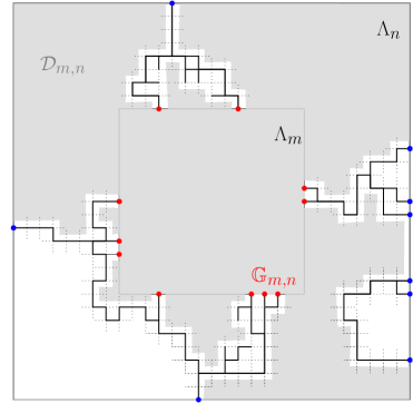
Figure 2: Description of a flower domain $\mathcal{D}_{m,n}$ (light grey area). The blue points are locations of spin changes (i.e. separation between sets $S_{i}$), the red points constitute $\mathbb{G}_{m,n}$, the solid black lines in the annulus $\Lambda_{n}\backslash\Lambda_{m}$ constitute ${\sf C}_{m,n}$.

3.2 Cardinality of $\mathbb{G}_{m,n}$

Flower domains have typically small sets $\mathbb{G}_{m,n}$, as the following proposition shows.

Proposition 3.1.

There exists $M>0$ such that for any $\delta>0$

$$\mu_{\Lambda_{n}}^{\sf f}\Bigl{(}\exists m\in\bigl{[}\tfrac{\delta n}{3},\delta n\bigr{]}:|\mathbb{G}_{m,n}|\leq M\Bigm{|}{\rm Cond}_{n}[\sigma]\Bigr{)}\geq 1-{\rm e}^{-\delta n},$$ (8)

uniformly in $\sigma$ and $n$ sufficiently large.

The notation $M$ will now be reserved for an integer $M>0$ satisfying the previous proposition. We shall prove this Proposition for $\delta=1$; the general case follows by a straightforward adaptation.

Definition 3.2.

Let $\mathcal{E}_{r}$ be the event that there exist $r$ disjoint crossings of $A_{n/3,n/2}$.

Lemma 3.3.

For all $r\geq 1$ and $n>0$,

$$\mu_{\Lambda_{n}}^{{\sf f}}(\mathcal{E}_{r})\leq{\rm e}^{-crn},$$

where $c>0$ is defined in Proposition 2.1.

Proof.

We prove that for all $r\geq 1$ and $n>0$,

$$\mu_{\Lambda_{n}}^{{\sf f}}(\mathcal{E}_{r})\leq\bigl{(}\mu^{{\sf w}}_{A_{n/3,n/2}}(\mathcal{E}_{1})\bigr{)}^{r}.$$ (9)

The conclusion will then follow easily, since Proposition 2.1 implies that $\mu^{{\sf w}}_{A_{n/3,n/2}}(\mathcal{E}_{1})\leq\exp(-cn)$.

In order to prove (9), we proceed by induction. First, note that $\mu_{\Lambda_{n}}^{{\sf f}}$ restricted to $A_{n/3,n/2}$ is stochastically dominated by $\mu_{A_{n/3,n/2}}^{{\sf w}}$.

Let $r\geq 1$ and consider $\mu_{\Lambda_{n}}^{{\sf f}}(\mathcal{E}_{r+1}|\mathcal{E}_{r})$. We number the vertices of $\partial\Lambda_{n}=\{x_{1},\ldots,x_{4n+4}\}$ in clockwise order, starting at the bottom right corner. Let $k$ be the smallest number such that there are $r$ crossings among the clusters containing $x_{1},\ldots,x_{k}$. Denote by $\mathcal{S}$ the union of these clusters (which may contain isolated vertices). Observe that all edges in $A_{n/3,n/2}\setminus\mathcal{S}$ which are incident to vertices of $\mathcal{S}$ are closed. Therefore, the conditional measure $\mu_{\Lambda_{n}}^{{\sf f}}(\cdot_{|A_{n/3,n/2}\setminus\mathcal{S}}|\mathcal{S})$ is stochastically dominated by $\mu^{\sf w}_{A_{n/3,n/2}}(\cdot_{|A_{n/3,n/2}\setminus\mathcal{S}})$. In both instances above, the symbol $\nu(\cdot_{|B})$ means the restriction of $\nu$ to edges of the graph with the vertex set $B$. As a result, the probability, under $\mu_{\Lambda_{n}}^{{\sf f}}(\cdot_{|A_{n/3,n/2}\setminus\mathcal{S}}|\mathcal{S})$, that there exists a crossing of $A_{n/3,n/2}$ is smaller than $\mu^{{\sf w}}_{A_{n/3,n/2}}(\mathcal{E}_{1})$. We obtain

$$\mu_{\Lambda_{n}}^{{\sf f}}(\mathcal{E}_{r+1}) =\mu_{\Lambda_{n}}^{{\sf f}}(\mathcal{E}_{r+1}|\mathcal{E}_{r})\mu_{\Lambda_{n}}^{{\sf f}}(\mathcal{E}_{r})=\mu_{\Lambda_{n}}^{{\sf f}}[\mu_{\Lambda_{n}}^{{\sf f}}(\mathcal{E}_{r+1}|\mathcal{S})]\mu_{\Lambda_{n}}^{{\sf f}}(\mathcal{E}_{r})$$

$$\leq\mu^{{\sf w}}_{A_{n/3,n/2}}(\mathcal{E}_{1})\mu_{\Lambda_{n}}^{{\sf f}}(\mathcal{E}_{r})\leq\mu^{{\sf w}}_{A_{n/3,n/2}}(\mathcal{E}_{1})^{r+1}.$$

∎

Proof of Proposition 3.1.

Obviously,

$$\mu_{\Lambda_{n}}^{\sf f}\bigl{(}\forall m\in\left[\tfrac{n}{3},\tfrac{n}{2}\right]:|\mathbb{G}_{m,n}|>M\bigm{|}{\rm Cond}_{n}[\sigma]\bigr{)}\leq\frac{\mu_{\Lambda_{n}}^{\sf f}\bigl{(}\forall m\in[\tfrac{n}{3},\tfrac{n}{2}]:|\mathbb{G}_{m,n}|>M\bigr{)}}{\mu_{\Lambda_{n}}^{\sf f}({\rm Cond}_{n}[\sigma])}.$$ (10)

Let us bound from below the denominator of (10). If all the edges of $\partial E_{n}$ are open, then ${\rm Cond}_{n}[\sigma]$ occurs. Moreover, the measure $\mu_{\Lambda_{n}}^{{\sf f}}$ stochastically dominates independent Bernoulli edge percolation on $\left\{0,1\right\}^{E_{n}}$ with $\tilde{p}=p/(p+(q-1)p)$, see [2, Theorem 4.1]. We deduce

$$\mu_{\Lambda_{n}}^{{\sf f}}({\rm Cond}_{n}[\sigma])\geq\mu_{\Lambda_{n}}^{{\sf f}}(\mbox{\rm all the edges in $\partial E_{n}$ are open})\geq\tilde{p}^{8n}.$$ (11)

Let us now bound from above the numerator of (10). First,

$$\mu_{\Lambda_{n}}^{{\sf f}}\bigl{(}\forall m\in\bigl{[}\tfrac{n}{3},\tfrac{n}{2}\bigr{]}:|\mathbb{G}_{m,n}|>M\bigr{)}\leq\mu_{\Lambda_{n}}^{{\sf f}}\bigl{(}|{\sf C}_{n/3,n}\cap A_{n/3,n/2}|\geq Mn/6\big{)}.$$

Fix $R>0$. If $|{\sf C}_{n/3,n}\cap A_{n/3,n/2}|\geq Mn/6$, either $A_{n/3,n/2}$ contains more than $R$ crossings or one of the crossings has cardinality larger than $Mn/(6R)$. Proposition 2.1 implies that the probability of having clusters with size larger than $Mn/(6R)$ in $\Lambda_{n/2}$ is smaller than $\exp[-cMn/(6R)]$ for $n$ large enough. Lemma 3.3 together with (10) implies that, for $n$ large enough,

$$\mu_{\Lambda_{n}}^{{\sf f}}\bigl{(}\forall m\in\bigl{[}\tfrac{n}{3},\tfrac{n}{2}\bigr{]}:|\mathbb{G}_{m,n}|>M\bigm{|}{\rm Cond}_{n}[\sigma]\bigr{)}\leq\tilde{p}^{-8n}[{\rm e}^{-cRn}+{\rm e}^{-cMn/(6R)}]\leq{\rm e}^{-n},$$

provided that $R$ and $M$ be sufficiently large. ∎

3.3 Reduction to FK measures on flower domains with free boundary condition

We define

$$\mathcal{M}_{n}=\max\{m\leq n:\left|\mathbb{G}_{m,n}\right|\leq M\},$$ (12)

where the maximum is set to be equal to $\infty$ if there is no $m\leq n$ such that $\left|\mathbb{G}_{m,n}\right|\leq M$. With this notation, we actually proved that $\mathcal{M}_{n}\in[\tfrac{n}{3},n]$ with probability bounded below by $1-{\rm e}^{-{n}}$.

Let $\mathcal{C}$ be a possible realization of ${\sf C}_{m,n}$ and $\mathcal{D}=\mathcal{D}_{m,n}$ be the corresponding flower domain. The restriction of $\mu_{\Lambda_{n}}^{{\sf f}}\left(\cdot~{}|~{}\mathcal{M}_{n}=m;{\sf C}_{m,n}=\mathcal{C}\right)$ to $\mathcal{D}$ is $\mu_{\mathcal{D}}^{\text{flower}}$. Furthermore,

$${\rm Cond}_{n}[\sigma]\cap\{\mathcal{M}_{n}=m\}\cap\{{\sf C}_{m,n}=\mathcal{C}\}$$

is a product event $\Omega_{\sigma,\mathcal{C}}\times\{\mathcal{M}_{n}=m;{\sf C}_{m,n}=\mathcal{C}\}$, where $\Omega_{\sigma,\mathcal{C}}\subset\left\{0,1\right\}^{\mathcal{E}_{\mathcal{D}}}$. Then

$$\mu_{\Lambda_{n}}^{{\sf f}}({\sf C}\cap\Lambda_{n^{\varepsilon}}\neq\varnothing\;|\;{\rm Cond}_{n}[\sigma];\mathcal{M}_{n}=m;{\sf C}_{m,n}=\mathcal{C})=\mu_{\mathcal{D}}^{\text{flower}}({\sf C}_{\mathbb{G}}\cap\Lambda_{n^{\varepsilon}}\neq\varnothing\,|\,\Omega_{\sigma,\mathcal{C}}).$$ (13)

The event $\Omega_{\sigma,\mathcal{C}}$ has an obvious structure. It corresponds to the existence of certain connections between different sites of $\mathbb{G}=\mathcal{C}\cap\partial\Lambda_{m}=\mathcal{D}\cap\partial\Lambda_{m}$. More precisely, let $\mathcal{P}_{\mathbb{G}}$ be the collection of different partitions of $\mathbb{G}$. Elements of $\mathcal{P}_{\mathbb{G}}$ are of the form $\underline{\mathbb{G}}=\left(\mathbb{G}_{1},\dots,\mathbb{G}_{\ell}\right)$. Define

$$\Omega_{\underline{\mathbb{G}}}=\bigcap_{i}\bigcap_{u,v\in\mathbb{G}_{i}}\{u\leftrightarrow v\}\subset\{0,1\}^{\mathcal{E}_{\mathcal{D}}}.$$

Let us say that a partition $\underline{\mathbb{G}}$ is compatible with $\Omega_{\sigma,\mathcal{C}}$ if $\Omega_{\underline{\mathbb{G}}}\subseteq\Omega_{\sigma,\mathcal{C}}$. Note that we do not rule out that some elements $\mathbb{G}_{i}$ of a partition $\underline{\mathbb{G}}$ are singletons. If $\mathbb{G}_{i}$ is a singleton, then $\bigcap_{u,v\in\mathbb{G}_{i}}\{u\leftrightarrow v\}$ is, of course, a sure event, which could be dropped from the definition of $\Omega_{\underline{\mathbb{G}}}$. In other words, only non-singleton elements of $\underline{\mathbb{G}}$ are relevant for $\Omega_{\underline{\mathbb{G}}}$. Also note that the events $\Omega_{\underline{\mathbb{G}}}$ do not have to be disjoint. Still, for any $\sigma$,

$$\Omega_{\sigma,\mathcal{C}}=\bigcup_{\underline{\mathbb{G}}\in\mathcal{P}^{\prime}_{\mathbb{G}}}\Omega_{\underline{\mathbb{G}}},$$

where the set $\mathcal{P}^{\prime}_{\mathbb{G}}$ corresponds to partitions which are compatible with the occurrence of the event $\Omega_{\sigma,\mathcal{C}}$, and which are maximal in the sense that one cannot find a finer partition which would be still compatible with $\Omega_{\sigma,\mathcal{C}}$.

The previous section implies the following reduction, which we will now consider for the rest of this work.

Proposition 3.4.

Fix $\delta>0$. Then, writing $B_{k}$ for the $k^{th}$ Bell number, which counts the number of partitions of a set of $k$ elements,

$$\mu_{\Lambda_{n}}^{{\sf f}}\bigl{(}{\sf C}\cap\Lambda_{n^{\varepsilon}}\neq\varnothing\bigm{|}{\rm Cond}_{n}[\sigma]\bigr{)}\leq{\rm e}^{-\delta n}+B_{M}q^{M}\max\mu_{\mathcal{D}}^{{\sf f}}\bigl{(}{\sf C}_{\mathbb{G}}\cap\Lambda_{n^{\varepsilon}}\neq\varnothing\bigm{|}\Omega_{\underline{\mathbb{G}}}\bigr{)},$$ (14)

for all boundary conditions $\sigma$ and $n$ sufficiently large. The above maximum is over all flower domains $\mathcal{D}$ rooted at $m\in[\tfrac{n}{3},n]$ with at most $\left|\mathbb{G}\right|\leq M$ marked points, and over all partitions $\underline{\mathbb{G}}\in\mathcal{P}^{\prime}_{\mathbb{G}}$.

Above the term $q^{M}$ comes from the fact that the elements of $\mathbb{G}$ are possibly wired together. It then bounds the Radon-Nikodym derivative between measures $\mu_{\mathcal{D}}^{\text{flower}}$ and $\mu_{\mathcal{D}}^{{\sf f}}$. The quantity $B_{M}$ bounds from above the number of sub-partitions of $\mathbb{G}$ (the events $\Omega_{\underline{\mathbb{G}}}$ being not necessarily disjoint).

4 Macroscopic structure near the center of the box

This section studies the macroscopic structure of the set ${\sf C}$ of sites connected to the boundary of $\Lambda_{n}$. Its main result, Proposition 4.2 below, implies that on a sufficiently small scale $\delta>0$, the intersection ${\sf C}\cap\Lambda_{k}$ for boxes with $k\in[\frac{\delta n}{3},\delta n]$ is with an overwhelming probability either empty, or close to a segment, or close to a tripod (three segments coming out from a point).

Before starting, note that Proposition 3.4 enables us to restrict attention to a flower domain $\mathcal{D}=\mathcal{D}_{m,n}$ with $m\in[\frac{n}{3},n]$ and $\left|\mathbb{G}_{m,n}\right|\leq M$. We set $\mathbb{G}=\mathbb{G}_{m,n}$. We now fix this flower domain and work under $\mu_{\mathcal{D}}^{{\sf f}}\left(\cdot~{}\big{|}~{}\Omega_{\underline{\mathbb{G}}}\right)$ for some $\underline{\mathbb{G}}\in\mathcal{P}_{\mathbb{G}}^{\prime}$. All constants in this section are independent of $\mathcal{D}_{m,n}$ and $\underline{\mathbb{G}}$ as long as $|\mathbb{G}_{m,n}|\leq M$. We will often recall this independence by using the expression “uniformly in $(\mathcal{D},\underline{\mathbb{G}})$ with $|\mathbb{G}|\leq M$”.

Define ${\sf C}_{k,\mathbb{G}}$ to be the set of edges connected to $\mathbb{G}$ in $\mathcal{D}\setminus\Lambda_{k}$ (which can consist of several connected components). Note that $\mathbb{G}_{k,n}={\sf C}_{k,n}\cap\partial\Lambda_{k}={\sf C}_{k,\mathbb{G}}\cap\partial\Lambda_{k}$. Given $v_{1},v_{2}\in\mathbb{R}^{2}$, we define $[v_{1},v_{2}]$ to be the line segment with endpoints $v_{1}$ and $v_{2}$, and $\measuredangle(v_{1},v_{2})$ to be the angle between $v_{1}$ and $v_{2}$, seen as vectors in the plane. We refer to Fig. 3 for an illustration of the following definitions.

Definition 4.1.

For $k<m$, $\nu>0$ and $\ell=1,2,3$, let us say that $E_{\nu,k}^{\ell}\subset\left\{0,1\right\}^{\mathcal{E}_{\mathcal{D}}}$ occurs if S$\ell$ below happens:

• $\mathbb{G}_{k,n}=\varnothing$.

• $\mathbb{G}_{k,n}=\mathbb{V}_{k,n}^{1}\cup\mathbb{V}_{k,n}^{2}$, where $\mathbb{V}_{k,n}^{1},\mathbb{V}_{k,n}^{2}$ are two disjoint sets of $\tau$-diameter less than or equal to $\nu k$. Moreover,

  • Each of the sets $\mathbb{V}_{k,n}^{1}$ and $\mathbb{V}_{k,n}^{2}$ is connected in ${\sf C}_{k,\mathbb{G}}$.

  • For any two vertices $v_{i}\in\mathbb{V}_{k,n}^{i}$; $i=1,2$, we have $[v_{1},v_{2}]\cap\Lambda_{k/2}\neq\varnothing$.

• $\mathbb{G}_{k,n}=\mathbb{V}_{k,n}^{1}\cup\mathbb{V}_{k,n}^{2}\cup\mathbb{V}_{k,n}^{3}$, where $\mathbb{V}_{k,n}^{1}$, $\mathbb{V}_{k,n}^{2}$ and $\mathbb{V}_{k,n}^{3}$ are disjoint sets with $\tau$-diameter less than or equal to $\nu k$. Moreover,

  • Each of the sets $\mathbb{V}_{k,n}^{1}$, $\mathbb{V}_{k,n}^{2}$ and $\mathbb{V}_{k,n}^{3}$ is connected in ${\sf C}_{k,\mathbb{G}}$,

  • For any choice of $v_{i}\in\mathbb{V}_{k,n}^{i};\ i=1,2,3$. there exists $x\in\Lambda_{k/2}$ such that $\mathcal{T}=\left\{v_{1},v_{2},v_{3};x\right\}$ is a Steiner tripod (see Definition 4.7 below). In particular, as it follows from P2 of Proposition 4.3 below, $\measuredangle(v_{i}-x,v_{j}-x)>\frac{\pi}{2}+\eta$ for every $i\neq j$ .

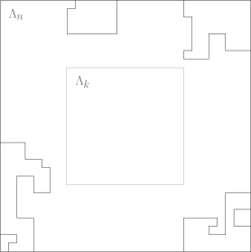
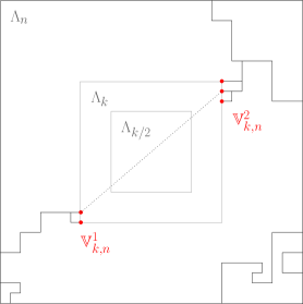
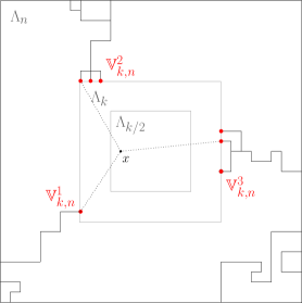
Figure 3: Description of the events $E^{\ell}_{\nu,k}$, $\ell=1,2,3$ from left to right. The set $\mathbb{G}_{k,n}$, partitioned into $\mathbb{V}^{\ell}_{k,n}$, $\ell=1,2,3$, is indicated in red.

We are now in a position to state the main proposition.

Proposition 4.2.

For any $\nu>0$, there exist $\delta=\delta(\nu,M)>0$ and $\kappa=\kappa(\nu,M)>0$ such that

$$\mu_{\mathcal{D}}^{{\sf f}}\Bigl{(}\ \bigcup_{k\geq\delta n}\big{(}E_{\nu,k}^{1}\cup E_{\nu,k}^{2}\cup E_{\nu,k}^{3}\big{)}\cap\big{\{}|\mathbb{G}_{k,n}|\leq M\big{\}}\ \Bigm{|}\ \Omega_{\underline{\mathbb{G}}}\ \Bigr{)}\geq 1-{\rm e}^{-\kappa n},$$ (15)

uniformly in $(\mathcal{D},\underline{\mathbb{G}})$ with $|\mathbb{G}|\leq M$.

The proof of Proposition 4.2 comprises two steps: First, we show that the implied geometric structure is characteristic of deterministic objects called Steiner forests. Then, we show that, with high $\mu_{\mathcal{D}}^{{\sf f}}(\,\cdot\,|\,\Omega_{\underline{\mathbb{G}}})$-probability, the cluster ${\sf C}_{\mathbb{G}}$ sits in the vicinity of one such forest.

4.1 Steiner forests

Note that for every $m$ the set $\mathcal{K}_{m}$ of all compact subsets of $\Lambda_{m}$ is a Polish space with respect to the ${\rm d}_{\tau}$-distance.

We now recall the concept of Steiner forest. Consider $E\subseteq\partial\Lambda_{m}$ with $|E|\leq M$. Let $\underline{E}=(E_{1},\dots,E_{i})$ be a partition of $E$ and $\Omega_{\underline{E}}$ be the set of compact subsets of $\mathbb{R}^{2}$ such that $E_{j}$ is included in one of their connected components for every $j\in\{1,\dots,i\}$. For the trivial partition $\underline{E}=\left\{E\right\}$, we shall write $\Omega_{E}$.

For a compact $\mathcal{S}\subset\mathbb{R}^{2}$, let $\tau(\mathcal{S})$ be the (one-dimensional) Hausdorff measure of $\mathcal{S}$ in the $\tau$-norm. Explicitly,

$$\tau(\mathcal{S})=\lim_{\varepsilon\to 0}\,\inf\Bigl{\{}\sum{\rm diam}_{\tau}(A_{i})\,:\,\mathcal{S}\subseteq\cup A_{i},\,{\rm diam}_{\tau}(A_{i})\leq\varepsilon\Bigr{\}},$$ (16)

where ${\rm diam}_{\tau}(A)=\sup\{\tau(x-y):x,y\in A\}$. Define the set of Steiner forests by

$$\Omega^{\rm min}_{\underline{E}}=\bigl{\{}\mathcal{F}\in\Omega_{\underline{E}}\,:\,\tau(\mathcal{F})=\min_{\mathcal{S}\in\Omega_{\underline{E}}}\tau(\mathcal{S})\bigr{\}}.$$

We set

$$\tau_{\underline{E}}=\min_{\mathcal{S}\in\Omega_{\underline{E}}}\tau(\mathcal{S})=\tau(\mathcal{F}),$$

for any Steiner forest $\mathcal{F}\in\Omega^{\rm min}_{\underline{E}}$.

In the sequel we shall work only with Steiner forests $\mathcal{F}\in\Omega^{\rm min}_{\underline{E}}$, when $\underline{E}$ is a partition of a set $E\subset\partial\Lambda_{m}$ of cardinality $\left|E\right|\leq M$. Let $\Omega^{\rm min}_{M,m}$ be the collection of all such forests.

Figure 4: A non trivial Steiner forest with a partition $\underline{E}=(E_{1},E_{2})$ with $E_{1}=\left\{u_{1},\dots,u_{4}\right\}$ and $E_{2}=\left\{u_{5},u_{6}\right\}$.

Proposition 4.3.

Fix $M>0$. The following properties hold uniformly in $m$, in finite subsets $E\subseteq\partial\Lambda_{m}$ with $|E|\leq M$ and in partitions $\underline{E}$ of $E$:

• (Number of Steiner forests and compactness of $\Omega^{\rm min}_{M,m}$) There exists $k=k(M)<\infty$ such that $|\Omega^{\rm min}_{\underline{E}}|\leq k$. The set $\Omega^{\rm min}_{M,m}$ is a compact subset of $\left(\mathcal{K}_{m},{\rm d}_{\tau}\right)$.

• (Structure of Steiner forests) The sets $\mathcal{F}\in\Omega^{\rm min}_{\underline{E}}$ are forests (that is collections of disjoint trees). Each inner node (that is not belonging to $E$) of such $\mathcal{F}$ has degree $3$. Furthermore, there exists an $\eta>0$ such that the angle between two edges incident to an inner node of $\mathcal{F}$ is always larger than $\tfrac{\pi}{2}+\eta$.

• (Well separateness of trees) There exists $\delta_{1}=\delta_{1}(M)>0$ such that any $\mathcal{F}\in\Omega^{\rm min}_{\underline{E}}$ satisfies:

  • for any Steiner tree $\mathcal{T}\in\mathcal{F}$, two different nodes of $\mathcal{T}$ in $\Lambda_{m/2}$ are at ${\rm d}_{\tau}$-distance at least $\delta_{1}m$ of each other;

  • if $\mathcal{T}_{1}$ and $\mathcal{T}_{2}$ are two disjoint trees of $\mathcal{F}$, then ${\rm d}_{\tau}\left(\mathcal{T}_{1}\cap\Lambda_{m/2},\mathcal{T}_{2}\cap\Lambda_{m/2}\right)\geq\delta_{1}m$ .

• (Stability) For any $\delta_{2}>0$, there exists $\kappa_{2}=\kappa_{2}(\delta_{2},M)>0$ such that, for any $\left|E\right|\leq M$, any partition $\underline{E}$ of $E$ and any $\mathcal{S}\in\Omega_{\underline{E}}$,

  $$\tau(\mathcal{S})\leq\tau_{\underline{E}}+\kappa_{2}m\quad\text{implies}\quad\min_{\mathcal{F}\in\Omega^{\rm min}_{M,m}}{\rm d}_{\tau}(\mathcal{S},\mathcal{F})<\delta_{2}m.$$ (17)

Proof.

We shall be rather sketchy since the arguments are presumably well understood. We shall consider the case $m=1$ (the general case follows by homogeneity).

Let us start with P4. The functional $\tau$ in (16) is lower semi-continuous on $(\mathcal{K}_{1},{\rm d}_{\tau})$ and has compact level sets (meaning sets of the form $\{\mathcal{S}:\tau(\mathcal{S})\leq R\}$). See, for instance, [14, Proposition 3.1], where these facts are explained for the inverse correlation length of sub-critical Bernoulli bond percolation.

Assume that P4 is wrong. Then there exists $\delta>0$ and two sequences; $\underline{E_{k}}$ and $\mathcal{S}_{k}\in\Omega_{\underline{E_{k}}}$, such that

$$\tau\left(\mathcal{S}_{j}\right)<\tau_{\underline{E_{k}}}+\frac{1}{k}\quad\text{but}\quad\min_{\mathcal{F}\in\Omega^{\rm min}_{M,m}}{\rm d}_{\tau}(\mathcal{S}_{j},\mathcal{F})>\delta.$$

Since $\left|E_{k}\right|\leq M$, the sequence $\tau_{\underline{E_{k}}}$ is bounded. Hence $\left\{\mathcal{S}_{j}\right\}$ is precompact. Possibly passing to subsequence we may assume that $\underline{E_{k}}$ converges to $\underline{E}$ (points might collapse, but this is irrelevant since this preserves $\left|E\right|\leq M$), and that $\mathcal{S}_{k}$ converges to $\mathcal{S}\in\Omega_{\underline{E}}$. Both convergence are, of course, in the sense of Hausdorff distance. By minimality it is evident that $\tau_{\underline{E}}=\lim\tau_{\underline{E_{k}}}$. By lower-semicontinuity $\tau(\mathcal{S})\leq\liminf\tau(\mathcal{S}_{k})$. Which means that $\mathcal{S}\in\Omega_{\underline{E}}^{\rm min}$. A contradiction.

A proof of the first assertion of P1 can be found in [12, Theorem 1]. Compactness of $\Omega_{M,1}^{\rm min}$ follows from compactness of level sets of $\tau$ and the fact that if $\mathcal{F}_{k}\in\Omega_{\underline{E_{k}}}^{\rm min}$ converges to $\mathcal{F}\in\Omega_{\underline{E}}$, then, as was already mentioned above, $\tau_{\underline{E}}=\lim\tau_{\underline{E_{k}}}$, and hence, by the lower-semicontinuity of $\tau$, $\mathcal{F}\in\Omega_{\underline{E}}^{\rm min}$.

A proof of P2 can be found in [5].

Let us turn to the proof of P3. For trivial partitions, Steiner forests are trees. Now, assume that there exists a sequence of Steiner trees $\mathcal{T}_{k}\in\Omega^{\rm min}_{{E}_{k}}$ such that $\mathcal{T}_{k}$ contains at least two inner nodes in $\Lambda_{1/2}$ at distance less or equal $\frac{1}{k}$. There is no loss of generality to assume that the sequence $\mathcal{T}_{k}$ converges to some $\mathcal{T}^{*}$ . As it follows from P4, $\mathcal{T}^{*}\in\Omega^{\rm min}_{{E}^{*}}$, where ${E}^{*}$ is the corresponding limit of ${E}_{k}$. Obviously, $|E^{*}|$ is still less or equal to $M$, since boundary points can only collapse under the limiting procedure.

The total number of nodes of each of $\mathcal{T}_{k}$ is uniformly bounded above. Hence by our assumption we can choose a number $\ell\geq 2$, a point $x\in\Lambda_{1/2}$, a radius $\varepsilon>0$ and a sequence $\nu(k)\to 0$, so that
(a) each of $\mathcal{T}_{k}$ contains $\ell$ nodes in $\Lambda_{\nu(k)}(x)=x+\Lambda_{\nu(k)}$;
(b) none of $\mathcal{T}_{k}$ contains nodes in the annulus $A_{\nu(k),\varepsilon}(x)$.
Then the restriction of $\mathcal{T}_{k}$ to $\Lambda_{\varepsilon}(x)$ is a Steiner tree, whereas the cardinality of the intersection ${|\partial\Lambda_{\varepsilon}(x)\cap\mathcal{T}_{k}|=\ell+2}$. By the minimality of $\mathcal{T}_{k}$ the points of $\partial\Lambda_{\varepsilon}(x)\cap\mathcal{T}_{k}$ are uniformly separated. Consequently, $|\partial\Lambda_{\varepsilon}(x)\cap\mathcal{T}^{*}|=\ell+2>3$. We infer that the degree of $x$ in the Steiner tree $\mathcal{T}^{*}$ is $\ell+2>3$, which is impossible by P2. This proves P3(a).

Consider now two disjoint Steiner trees $\mathcal{T}_{1}\in\Omega^{\rm min}_{{E}_{1}}$ and $\mathcal{T}_{2}\in\Omega^{\rm min}_{{E}_{2}}$, such that the forest $\left\{\mathcal{T}_{1},\mathcal{T}_{2}\right\}$ belongs to $\Omega^{\rm min}_{\left\{{E}_{1},E_{2}\right\}}$. By the strict convexity of $\tau$, the trees are confined to their convex envelopes: $\mathcal{T}_{i}\in{\rm co}\left(E_{i}\right)$ for $i=1,2$. Thus if both trees are disjoint and intersect $\Lambda_{1/2}$, it follows that ${\rm co}\left(E_{1}\right)\cap{\rm co}\left(E_{2}\right)=\varnothing$. Consequently, there exist $u_{1},v_{1}\in E_{1}$ and $u_{2},v_{2}\in E_{2}$, such that $\mathcal{T}_{1}$ lies below the interval $[u_{1},v_{1}]$ and $\mathcal{T}_{2}$ lies above the interval $[u_{2},v_{2}]$ (notions of above and below are with respect to the directions of normals). We are now facing two cases:

• $\mathcal{T}_{1}$ or $\mathcal{T}_{2}$ has an inner node in $\Lambda_{2/3}$. By P2, inner nodes are of degree three and angles between edges incident to inner nodes are at most $\pi-2\eta$. This pushes inner nodes of $\mathcal{T}_{i}$ away from $[u_{i},v_{i}]$ uniformly in $\mathcal{T}_{1}$ and $\mathcal{T}_{2}$. In such a case, P3 is satisfied.

• Both $\mathcal{T}_{1}$ and $\mathcal{T}_{2}$ do not contain nodes in $\Lambda_{2/3}$, but each contains an edge which crosses $\Lambda_{1/2}$. Having such edges close to each other (and hence running essentially in parallel across $\Lambda_{1/2}$) is easily seen to be incompatible with the minimality of $\mathcal{F}$.

This achieves the proof of P3(b). ∎

4.2 Forest skeleton of the cluster ${\sf C}_{\mathbb{G}}$

Let $\underline{\mathbb{G}}$ be a partition of $\mathbb{G}$. We now aim to show that, under $\mu_{\mathcal{D}}^{{\sf f}}(\,\cdot\,|\,\Omega_{\underline{\mathbb{G}}})$, the cluster ${\sf C}_{\mathbb{G}}$ stays typically close to one of the Steiner forests from $\Omega_{M,m}^{\rm min}$. In order to do that, we introduce the notion of forest skeleton of the cluster. This notion is a modification of the coarse-graining procedure developed in Section 2.2 of [10].

Let ${\mathbf{U}}_{\tau}$ be the unit ball in $\tau$-norm. Fix a large number $c>0$ and consider $K$ such that $c\log K<K$. For any $y\in\Z^{2}$, set

$${\mathbf{B}}_{K}(y)\,=\,\left(y+K\cdot{\mathbf{U}}_{\tau}\right)\cap\Z^{2}\quad\text{and}\quad\hat{\mathbf{B}}_{K}(y)\,=\,{\mathbf{B}}_{K+c\log K}(y).$$

If $x\in A\subset\Z^{2}$ and $y\in A\cup\partial^{{{\rm ext}}}A$, we shall use $\{x\stackrel{{\scriptstyle A}}{{\longleftrightarrow}}y\}$ to denote the event that $x$ and $y$ are connected by an open path from $x$ to $y$ whose vertices belong to $A$, with the possible exception of the terminal point $y$ itself.

Let us construct the forest skeleton $\mathcal{F}_{K}$ of the cluster ${\sf C}_{\mathbb{G}}$ (see Figure 5). Here and below, vertices in $\Z^{2}$ are ordered using the lexicographical ordering. In the following construction, we will often refer to the minimal vertex having some property.

Step 1. Set $r=1,i=1$. Set $x_{0}^{1}=u_{i_{1}}$ be the minimal vertex of $\mathbb{G}$. Set $V=\left\{x_{0}^{1}\right\}$ and $\mathcal{C}=\hat{\mathbf{B}}_{K}(x_{0}^{1})$. Go to Step 2.

Step 2. If there exists $x\in V$ and $u\in\mathbb{G}\setminus V$ such that $u\in\hat{\mathbf{B}}_{2K}(x)$, then choose $u^{*}\in\mathbb{G}\setminus V$ to be the minimal such vertex. Set $x^{r}_{i}=u^{*},{A_{i}^{r}={\mathbf{B}}_{K}(x_{i}^{r})}$ and go to Step 3. Otherwise, go to Step 4.

Step 3. Update $V\rightarrow V\cup\{x_{i}^{r}\}$, $\mathcal{C}\to\mathcal{C}\cup\hat{\mathbf{B}}_{K}(x_{i}^{r})$ and $i\to i+1$. Go to Step 2.

Step 4. If there is at least one vertex $y\in\partial^{{\rm ext}}\mathcal{C}$ such that

$$y\stackrel{{\scriptstyle{\sf C}_{\mathbb{G}}\setminus\mathcal{C}}}{{\longleftrightarrow}}\partial^{{\rm ext}}{\mathbf{B}}_{K}(y)\setminus\mathcal{C},$$

then choose $y^{*}$ to be the minimal such vertex, set $x_{i}^{r}=y^{*},A_{i}^{r}={\mathbf{B}}_{K}(x_{i}^{r})\setminus\mathcal{C}$, and go to Step 3. Otherwise, go to Step 5.

Step 5. If $\mathbb{G}\subset V$, then terminate the construction. Otherwise, choose $u^{*}$ to be the minimal vertex of $\mathbb{G}\setminus V$. Update $r\to r+1$ and set $x_{0}^{r}=u^{*}$. Update $V\to V\cup\left\{x_{0}^{r}\right\}$ and $i=1$. Go to Step 2.

Definition 4.4.

The above procedure produces $r$ disjoint sets of vertices $V^{1}=\left\{x_{0}^{1},x_{1}^{1},\dots\right\}$, $V^{2}=\left\{x_{0}^{2},x_{1}^{2},\dots\right\}$, $\dots$, $V^{r}=\left\{x_{0}^{r},x_{1}^{r},\dots\right\}$. The vertices $x_{i}^{j}$ constructed on Step 4 are equipped with sets $A_{i}^{j}$, $j=1\ldots r$. Exit paths through such $A_{i}^{j}$-s contribute multiplicative factors ${\rm e}^{-K}$ each. Sets $A_{i}^{j}$ for vertices $x_{i}^{j}$ constructed on Step 2 play no role and are introduced for notational convenience only (see (4.3) below). By construction, there are at most $M$ such vertices.

The edges within each group $\ell=1,\dots,r$ are constructed as follows: $x_{i}^{\ell}$ is connected to the vertex of

$$\bigl{\{}x_{j}^{\ell}\,:\,j<i\text{ and }x_{i}\in\hat{\mathbf{B}}_{2K}(x_{j})\bigr{\}}$$

which has smallest index $j$.

This produces a graph which is a set of $r$ trees $\mathcal{T}_{K}^{1},\ldots,\mathcal{T}_{K}^{r}$. The union of the trees is called the forest skeleton $\mathcal{F}_{K}=\cup_{\ell}\mathcal{T}_{K}^{\ell}$.

Note that we consider these graphs as compact subsets of $\mathbb{R}^{2}$. An example of forest squeleton is drawn on Figure 5. The following result follows trivially from the construction of the forest skeleton.

Proposition 4.5.

Let $\mathcal{F}_{K}$ be the forest skeleton of ${\sf C}_{\mathbb{G}}$, then

1. $\mathbb{G}$ is included in the vertices of $\mathcal{F}_{K}$.

2. Two vertices $u,v\in\mathbb{G}$ which were connected in ${\sf C}_{\mathbb{G}}$ are also connected in $\mathcal{F}_{K}$.

3. ${\sf C}_{\mathbb{G}}\subseteq\cup_{\ell,i}\hat{\mathbf{B}}_{2K}(x_{i}^{\ell})$.

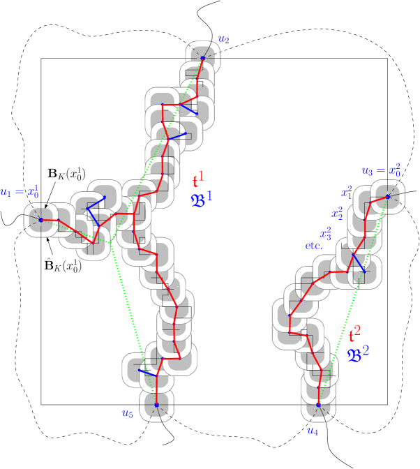
Figure 5: Construction of the forest skeleton $\mathcal{F}_{K}=\{\mathcal{T}_{K}^{1},\mathcal{T}_{K}^{2}\}$ of the cluster ${\sf C}_{\mathbb{G}}$ (in black), consisting of the trees $\mathcal{T}_{K}^{i}=\{\mathfrak{t}^{i},\mathfrak{B}^{i}\}$, $i=1,2.$ The Steiner forest corresponding to the partition $\underline{\mathbb{G}}=(\{u_{1},u_{2},u_{5}\},\{u_{3},u_{4}\})$ is drawn in dashed green.

4.3 Distance between ${\sf C}_{\mathbb{G}}$ and Steiner forests

Proposition 4.6.

For every $\delta_{3}>0$, there exists $\kappa_{3}=\kappa_{3}(M)>0$ such that for $n$ large enough,

$$\mu_{\mathcal{D}}^{\sf f}\Bigl{(}\min_{\mathcal{F}\in\Omega^{\rm min}_{M,m}}{\rm d}_{\tau}\bigl{(}{\sf C}_{\mathbb{G}},\mathcal{F}\bigr{)}>\delta_{3}n\Bigm{|}\Omega_{{\underline{\mathbb{G}}}}\Bigr{)}\leq{\rm e}^{-\kappa_{3}n},$$

uniformly in $(\mathcal{D},\underline{\mathbb{G}})$ with $|\mathbb{G}|\leq M$.

Proof.

Let $\mathcal{F}_{K}$ be the forest skeleton of ${\sf C}_{\mathbb{G}}$ at scale $K$ ($K$ will be chosen later). By the third item of Proposition 4.5,

$$\mathrm{d}_{\tau}\left({\sf C}_{\mathbb{G}},\mathcal{F}_{K}\right)\leq 2K+c\log 2K.$$

The proposition thus reduces to the following claim: for any $\delta_{3}>0$, there exist $K=K(M)>0$ and $\kappa_{3}=\kappa_{3}(M)>0$ such that

$$\mu_{\mathcal{D}}^{\sf f}\Bigl{(}\min_{\mathcal{F}\in\Omega^{\rm min}_{M,m}}{\rm d}_{\tau}\bigl{(}\mathcal{F}_{K},\mathcal{F}\bigr{)}>\delta_{3}n\Bigm{|}\Omega_{{\underline{\mathbb{G}}}}\Bigr{)}\leq{\rm e}^{-\kappa_{3}n},$$

uniformly in $(\mathcal{D},\underline{\mathbb{G}})$ with $|\mathbb{G}|\leq M$. We now prove this statement.

Writing $E:=\{\min_{\mathcal{F}\in\Omega^{\rm min}_{M,m}}{\rm d}_{\tau}\bigl{(}\mathcal{F}_{K},\mathcal{F}\bigr{)}>\delta_{3}n\}$, we have

$$\mu_{\mathcal{D}}^{\sf f}(E|\Omega_{{\underline{\mathbb{G}}}})=\frac{\mu_{\mathcal{D}}^{\sf f}(E\cap\Omega_{{\underline{\mathbb{G}}}})}{\mu_{\mathcal{D}}^{\sf f}(\Omega_{{\underline{\mathbb{G}}}})}\leq\frac{\mu_{\mathcal{D}}^{\sf f}(\tau(\mathcal{F}_{K})\geq\tau_{{\mathbb{G}}}+\kappa_{2}n)}{\mu_{\mathcal{D}}^{\sf f}(\Omega_{{\underline{\mathbb{G}}}})}$$ (18)

where in the last inequality we used Property P4 of Proposition 4.3, applied with $\delta_{2}=\delta_{3}$.

Let $\mathcal{F}$ be a Steiner forest in $\Omega_{\underline{\mathbb{G}}}^{\rm min}$ and $\mathcal{F}^{\prime}$ be the forest obtained by replacing each inner node of $\mathcal{F}$ by the closest vertex of $\Z^{2}$. Now, by the FKG inequality, we can lower bound the denominator

$$\mu_{\mathcal{D}}^{\sf f}(\Omega_{{\underline{\mathbb{G}}}}) \geq\mu_{\mathcal{D}}^{\sf f}\Bigl{(}\bigcap_{\{x,y\}\in\mathcal{E}(\mathcal{F}^{\prime})}\{x\leftrightarrow y\}\Bigr{)}\geq\prod_{\{x,y\}\in\mathcal{E}(\mathcal{F}^{\prime})}\mu_{\mathcal{D}}^{\sf f}(x\leftrightarrow y)$$

$$\geq\prod_{\{x,y\}\in\mathcal{E}(\mathcal{F}^{\prime})}{\rm e}^{-\tau(y-x)(1+o_{\left|y-x\right|}(1))}={\rm e}^{-\tau_{\mathbb{G}}(1+o_{n}(1))}.$$ (19)

where $\lim_{k\to\infty}{\mathrm{o}}_{k}(1)=0$ by definition, and the product is taken over the set $\mathcal{E}(\mathcal{F}^{\prime})$ of all the inner edges of the approximate Steiner forest $\mathcal{F}^{\prime}$.

To obtain an upper bound on the numerator, we follow [10, Section 2]. Let $|V(\mathcal{F}_{{K}})|=\sum_{\ell=1}^{r}|V^{\ell}|$ be the total number of vertices of the forest skeleton $\mathcal{F}$, then

$${{\rm e}^{-2KM}}\mu_{\mathcal{D}}^{\sf f}(\mathcal{F}_{K}=\mathcal{F}) \leq\mu_{\mathcal{D}}^{\sf f}\Bigl{(}\bigcap_{\ell=1}^{r}\bigcap_{i=0}^{|V^{\ell}|}x_{i}^{\ell}\stackrel{{\scriptstyle{A_{i}^{\ell}}}}{{\leftrightarrow}}\partial^{{{\rm ext}}}{\mathbf{B}}_{K}(x_{i}^{\ell})\Bigr{)}\leq\prod_{\ell=1}^{r}\prod_{i=1}^{|V^{\ell}|}\mu_{\hat{A}_{K}^{i}}^{\sf w}\bigl{(}x_{i}^{\ell}\stackrel{{\scriptstyle{A_{i}^{\ell}}}}{{\leftrightarrow}}\partial^{{{\rm ext}}}{\mathbf{B}}_{K}(x_{i}^{\ell})\bigr{)}$$

$$\leq\bigl{(}{\rm e}^{-K(1-{\mathrm{o}}_{K}(1))}\bigr{)}^{\sum_{\ell=1}^{r}|V^{\ell}|}={\rm e}^{-K|V(\mathcal{F})|(1-{\mathrm{o}}_{K}(1))}$$

$$\leq{\rm e}^{-\tau(\mathcal{F})(1-{\mathrm{o}}_{K}(1)-{\mathrm{o}}_{n}(1))},$$ (20)

where in the first inequality the term ${\rm e}^{-2MK}$ compensates (by the FKG inequality) the inclusion of events $x_{i}^{\ell}\stackrel{{\scriptstyle{A_{i}^{\ell}}}}{{\leftrightarrow}}\partial^{{{\rm ext}}}{\mathbf{B}}_{K}(x_{i}^{\ell})$ for points $x_{i}^{\ell}\in\mathbb{G}$, whereas in the second inequality we expand the probability of the intersection as a product of conditional expectations and then use the FKG inequality to compare this conditional expectations with the probability with wired boundary conditions, and in the second line we use that $\mu_{{\mathbf{B}}_{K}(x)}^{\sf w}(x\leftrightarrow\partial^{{{\rm ext}}}{\mathbf{B}}_{K}(x))={\rm e}^{-K(1-{\mathrm{o}}_{K}(1))}$ (this follows from [10, Corollary 1.1], which is now known to be valid up to $p_{c}(q)$ thanks to Proposition 2.1). If we now upper bound crudely the number of forest $K$-skeletons rooted at $\mathbb{G}$ with $\tau(\mathcal{F})=T$ (and so with less than $C_{1}T/K$ vertices) by $(C_{2}K)^{C_{3}T/K}$, we get

$$\mu_{\mathcal{D}}^{\sf f}(\tau(\mathcal{F}_{K})\geq\tau_{{\mathbb{G}}}+\kappa_{2}n) =\sum_{\mathcal{F}:\tau(\mathcal{F})\geq\tau_{\mathbb{G}}+\kappa_{2}n}\mu_{\mathcal{D}}^{\sf f}(\mathcal{F}_{K}=\mathcal{F})=\sum_{T\geq\tau_{\mathbb{G}}+\kappa_{2}n}\sum_{\begin{subarray}{c}\mathcal{F}\;:\\ \tau(\mathcal{F})=T\end{subarray}}\mu_{\mathcal{D}}^{\sf f}(\mathcal{F}_{K}=\mathcal{F})$$

$$=\sum_{T\geq\tau_{\mathbb{G}}+\kappa_{2}n}{\rm e}^{(C_{1}T/K)\log(C_{2}K)-T(1-{\mathrm{o}}_{K}(1)-{\mathrm{o}}_{n}(1))}$$

$$\leq C_{4}\cdot{\rm e}^{-(\tau_{\mathbb{G}}+\kappa_{2}n)(1+{\mathrm{o}}_{K}(1)+{\mathrm{o}}_{n}(1))},$$ (21)

where we used (4.3) in the second line. The result follows by comparison with (4.3):

$$\mu_{\mathcal{D}}^{\sf f}(E|\Omega_{\mathbb{G}})\leq{\rm e}^{-(\tau_{\mathbb{G}}+\kappa_{2}n)(1-{\mathrm{o}}_{K}(1)-{\mathrm{o}}_{n}(1))+\tau_{\mathbb{G}}(1+{\mathrm{o}}_{n}(1))}\leq{\rm e}^{-n\kappa_{3}}.$$

Note that $\tau_{\mathbb{G}}o_{n}(1)=o(n)$ since $\tau_{\mathbb{G}}=O(n)$. The latter follows from the fact that $\tau_{\mathbb{G}}$ is bounded by the $\tau$-length of the forest obtained by opening all the edges of $\partial E_{m}$ (recall that $\tau$ is an equivalent norm on $\mathbb{R}^{2}$). ∎

Proof of Proposition 4.2.

Fix $\mathcal{D}=\mathcal{D}_{m,n}$ and $\mathbb{G}=\mathbb{G}_{m,n}$ with $m\geq\frac{n}{3}$ and $|\mathbb{G}|\leq M$. Let $\nu>0$. Fix an arbitrary $0<\delta\ll 1$ such that $\Lambda_{250\delta n}\subset\delta_{1}n\mathbf{U}_{\tau}$, where $\delta_{1}$ is given by P3. By definition of $\delta$, we know that for any forest $\mathcal{F}\in\Omega^{\rm min}_{{M},m}$, $\mathcal{F}\cap\Lambda_{250\delta n}$ is connected and contains at most one node. Therefore, we have three cases: either $\mathcal{F}\cap\Lambda_{2\delta n}=\varnothing$, or $\mathcal{F}\cap\Lambda_{2\delta n}\neq\varnothing$ but $\mathcal{F}\cap\Lambda_{20\delta n}$ contains only one edge, or $\mathcal{F}\cap\Lambda_{20\delta n}$ contains more than one edge. In the later case, the fact that edges incident to a node make an angle larger or equal to $\frac{\pi}{2}+\eta$ implies that $\mathcal{F}\cap\Lambda_{40\delta n}$ contains a node.

Also set $\delta_{3}<\min\{\nu,\delta\}$. Proposition 4.6 implies that

$$\min_{\mathcal{F}\in\Omega^{\rm min}_{M,m}}\mathrm{d}_{\tau}\bigl{(}{\sf C}_{\mathbb{G}},\mathcal{F}\bigr{)}\leq\delta n,$$ (22)

with probability larger than $1-{\rm e}^{-\kappa_{3}n}$ for $n$ large enough. We now assume that this inequality is indeed satisfied. Since, by P1 of Proposition 4.3 the set $\Omega^{\rm min}_{M,m}$ is compact, and since we are after an upper bound which vanishes with $n$, it will be enough to fix a Steiner forest $\mathcal{F}\in\Omega^{\rm min}_{M,m}$ and to assume that

$$\mathrm{d}_{\tau}\bigl{(}{\sf C}_{\mathbb{G}},\mathcal{F}\bigr{)}\leq\delta n,$$ (23)

Let us treat the three previous cases separately.

• $\mathcal{F}\cap\Lambda_{2\delta n}=\varnothing$. In such case, (23) shows that ${\sf C}_{\mathbb{G}}\cap\Lambda_{\delta n}=\varnothing$. Thus, $E^{1}_{\nu,\delta n}$ holds true and $\mathbb{G}_{\delta n,n}=\varnothing$.

• $\mathcal{F}\cap\Lambda_{20\delta n}=[u_{1},u_{2}]$ with $u_{1}$ and $u_{2}$ on $\partial\Lambda_{20\delta n}$ and $[u_{1},u_{2}]\cap\Lambda_{2\delta n}\neq\varnothing$. In such case, (23) shows that ${\sf C}_{\mathbb{G}}$ intersects $\Lambda_{3\delta n}$ which in turns implies that $E^{2}_{\nu,k}$ holds for every $k\in[6\delta n,18\delta n]$. Proposition 3.1 implies the existence of $k\in[6\delta n,18\delta n]$ with $|\mathbb{G}_{k,n}|\leq M$ on an event of probability larger than $1-{\rm e}^{-18\delta n}$.

• There exists a node $x\in\Lambda_{40\delta n}$ and therefore $\mathcal{F}\cap\Lambda_{250\delta n}=[u_{1},x]\cup[u_{2},x]\cup[u_{3},x]$ with $u_{1}$, $u_{2}$, $u_{3}$ on $\partial\Lambda_{250\delta n}$ such that $\measuredangle(u_{i}-x,u_{j}-x)>\frac{\pi}{2}+\eta$ for every $i\neq j$. In such case, (23) shows that $E^{3}_{\nu,k}$ holds for every $k\in[82\delta n,246\delta n]$. Proposition 3.1 implies the existence of $k\in[82\delta n,246\delta n]$ with $|\mathbb{G}_{k,n}|\leq M$ on an event of probability larger than $1-{\rm e}^{-246\delta n}$.

Altogether, we obtain the claim. ∎

For later use, let us introduce the following definition:

Definition 4.7.

For $u_{1},u_{2},u_{3}$ in general position the function $\phi(y):=\sum_{i=1}^{3}\tau(u_{i}-y)$ is strictly convex and quadratic around its minimum point; see [9, Lemma 3]. Let $x$ be the unique minimizer of $\phi$. In this way the notation $\mathcal{T}(u_{1},u_{2},u_{3};x)$ is reserved for the minimal Steiner forest (in this case it is a tree) which contains $u_{1},u_{2},u_{3}$. It might happen, of course, that $x$ coincides with one of the $u_{i}$-s. When, however, this is not the case, we shall refer to $\mathcal{T}(u_{1},u_{2},u_{3};x)$ as a Steiner tripod.

5 Fluctuation theory and proof of Theorem 2.2

We are now in a position to prove Theorem 2.2. Let $\nu>0$ small enough to be fixed later. By (14) and (15), we can assume that there exist $\delta=\delta(\nu)>0$ and $k\geq\delta n$ such that $|\mathbb{G}_{k,n}|\leq M$ and $E^{\ell}_{\nu,k}$ holds true for some $\ell\in\{1,2,3\}$. Let

$$\mathcal{R}_{n}=\max\left\{k\geq\delta n:|\mathbb{G}_{k,n}|\leq M\text{ and }E^{1}_{\nu,k}\cup E^{2}_{\nu,k}\cup E^{3}_{\nu,k}\right\}\in\left[\delta n,n\right].$$

Let $\mathcal{C}$ be a possible realization of ${\sf C}_{k,n}$ and $\mathcal{D}=\mathcal{D}_{k,n}$ be the corresponding flower domain. We also set $\mathbb{G}=\mathbb{G}_{k,n}$. The restriction of $\mu_{\Lambda_{n}}^{{\sf f}}\left(\cdot~{}|~{}\mathcal{R}_{n}=k;{\sf C}_{k,n}=\mathcal{C}\right)$ to $\mathcal{D}$ is $\mu_{\mathcal{D}}^{\text{flower}}$. Exactly as in Section 3.3,

$${\rm Cond}_{n}[\sigma]\cap\{\mathcal{R}_{n}=k\}\cap\{{\sf C}_{k,n}=\mathcal{C}\}=\Omega_{\sigma,\mathcal{C}}\times\{\mathcal{R}_{n}=k;{\sf C}_{k,n}=\mathcal{C}\},$$

where $\Omega_{\sigma,\mathcal{C}}=\cup_{\underline{\mathbb{G}}\in\mathcal{P}^{\prime}_{\mathbb{G}}}\Omega_{\underline{\mathbb{G}}}$ is defined as in Section 3.3. This reduction shows that it is sufficient to prove that

$$\mu^{\sf f}_{\mathcal{D}}\bigl{(}{\sf C}_{\mathbb{G}}\cap\Lambda_{n^{\varepsilon}}\neq\varnothing\bigm{|}\Omega_{\sigma,\mathcal{C}}\bigr{)}=O(n^{\varepsilon-1/2}),$$

uniformly in the possible realizations of $\mathcal{D}$, $\mathcal{C}$ and $\mathbb{G}$.

From now on, we fix $k\geq\delta n$ such that $|\mathbb{G}_{k,n}|\leq M$ and $E^{\ell}_{\nu,k}$ holds true for some $\ell\in\{1,2,3\}$. We set $\mathcal{D}=\mathcal{D}_{k,n},{\mathcal{C}=\mathcal{C}_{k,n}}$ and $\mathbb{G}=\mathbb{G}_{k,n}$.

Since each set $\mathbb{V}^{i}$ is already assumed to be connected outside of $\mathcal{D}$ (since $E^{1}_{\nu,k}\cup E^{2}_{\nu,k}\cup E^{3}_{\nu,k}$ occurs), partitions $\underline{\mathbb{G}}\in\mathcal{P}^{\prime}_{\mathbb{G}}$ can be of four different types (recall that they are maximal in the sense defined in the previous section): singletons only, singletons together with one pair of elements in two different $\mathbb{V}^{i}$ (this cannot occur in $E^{1}_{\nu,k}$), singletons together with one triplet of elements in three different $\mathbb{V}^{i}$ (this can occur only in $E^{3}_{\nu,k}$), singletons together with two pairs $(u,v)$ and $(u^{\prime},w)$, where $u$ and $u^{\prime}$ belong to the same $\mathbb{V}^{i}$, and $v$ and $w$ belong to the other $\mathbb{V}^{j}$ (this can occur only in $E^{3}_{\nu,k}$). Let $\mathcal{P}^{*}_{\mathbb{G}}$ be the set of partitions in $\mathcal{P}^{\prime}_{\mathbb{G}}$ of one of the first three types. If the configuration is in $\Omega_{\sigma,\mathcal{C}}\setminus\cup_{\underline{\mathbb{G}}\in\mathcal{P}^{*}_{\mathbb{G}}}\Omega_{\underline{\mathbb{G}}}$, there are two different clusters connecting two pairs of vertices $(u,v)$ and $(u^{\prime},w)$ satisfying the conditions described above. By choosing $\nu>0$ small enough, the assumption that $E^{3}_{\nu,k}$ holds implies that $\tau(u-v)+\tau(u^{\prime}-w)\geq(1+\varepsilon)\tau_{\mathbb{G}}$ (where $\varepsilon=\varepsilon(\delta_{3},\nu)>0$) uniformly in the possible pairs $(u,v)$ and $(u^{\prime},w)$. As in the proof of Proposition 4.6, one obtains after a small computation that

$$\mu^{\sf f}_{\mathcal{D}}\bigl{(}\Omega_{\sigma,\mathcal{C}}\setminus\cup_{\underline{\mathbb{G}}\in\mathcal{P}^{*}_{\mathbb{G}}}\Omega_{\underline{\mathbb{G}}}\bigm{|}\Omega_{\sigma,\mathcal{C}}\bigr{)}=O({\rm e}^{-ck}),$$

for some constant $c>0$. Hence, a reduction in the spirit of Proposition 3.4 shows that Theorem 2.2 would follow from the bound

$$\mu^{\sf f}_{\mathcal{D}}\bigl{(}{\sf C}_{\mathbb{G}}\cap\Lambda_{n^{\varepsilon}}\neq\varnothing\bigm{|}\Omega_{\underline{\mathbb{G}}}\bigr{)}=O(n^{\varepsilon-1/2}),$$ (24)

where the right-hand side is uniform in the possible realizations of $\mathcal{D}$ and in the $\underline{\mathbb{G}}\in\mathcal{P}^{*}_{\mathbb{G}}$. We decompose the proof of (24) into three cases, depending on the type of $\underline{\mathbb{G}}$.

Scenario S1: No imposed crossing.

This occurs in the following two cases (cf. Definition (4.1)): (i) $E^{1}_{\nu,k}$ occurs; (ii) $E^{2}_{\nu,k}\cup E^{3}_{\nu,k}$ occurs and the partition $\underline{\mathbb{G}}$ is composed of singletons only. In this case, the measure $\mu^{\sf f}_{\mathcal{D}_{k,n}}(\,\cdot\,|\Omega_{\underline{\mathbb{G}}})$ is unconditioned (i.e. $\Omega_{\underline{\mathbb{G}}}=\Omega$). Proposition 2.1 then implies that $\mu^{\sf f}_{\mathcal{D}}\bigl{(}{\sf C}_{\mathbb{G}}\cap\Lambda_{n^{\varepsilon}}\neq\varnothing\bigm{|}\Omega_{\underline{\mathbb{G}}}\bigr{)}$ decays exponentially with $n$.

Scenario S2: One imposed crossing.

This occurs when $E^{2}_{\nu,k}\cup E^{3}_{\nu,k}$ occurs and $\underline{\mathbb{G}}$ is composed of singletons together with a unique pair $(u,v)$, where $u\in\mathbb{V}^{i},v\in\mathbb{V}^{j}$ with $i\neq j$. In other words, $\Omega_{\underline{\mathbb{G}}}=\left\{u\leftrightarrow v\right\}$. In this case, the cluster $\mathcal{C}_{\mathbb{G}}\subseteq\mathcal{D}$ may contain several connected components, but, up to exponentially small (in $k$) $\mu^{\sf f}_{\mathcal{D}}(\cdot|u\leftrightarrow v)$-conditional probabilities, only one of them, namely the connected cluster ${\sf C}(u,v)$ of $\left\{u,v\right\}$ is capable of reaching $\Lambda_{n^{\varepsilon}}$. However, the law of the cluster connecting $u$ and $v$ converges to the law of a Brownian bridge. In fact, one obtains the following stronger result:

$$\mu^{\sf f}_{\mathcal{D}}(x\in{\sf C}(u,v)|u\leftrightarrow v)\leq\frac{C}{\sqrt{|u-v|}}\exp\Bigl{(}-\kappa\frac{d_{\tau}(x,[u,v])^{2}}{|u-v|}\Bigr{)},$$ (25)

where $\kappa$ and $C$ are constants depending on $p$ only, and $[u,v]$ denotes the segment between $u$ and $v$. In the case of Ising interfaces, such bound was obtained in [22, (3.31)]. The proof relies on the positive curvature of the surface tension and on the effective random walk with exponentially decaying step distribution representation of the interface. The theory developed in [10] enables a literal adaptation to the case of sub-critical FK-clusters, see Theorems C and E and Subsections 4.4 and 4.5 in [10]. Consequently,

$$\mu_{\mathcal{D}}^{{\sf f}}\bigl{(}{\sf C}_{\mathbb{G}}\cap\Lambda_{n^{\varepsilon}}\neq\varnothing\bigm{|}\Omega_{\underline{\mathbb{G}}}\bigr{)}=O(n^{2\varepsilon-1/2}).$$ (26)

Scenario S3: One tripod.

This can only happen when $E^{3}_{\nu,k}$ occurs and $\underline{\mathbb{G}}$ is composed of singletons together with one triplet $(u_{1},u_{2},u_{3})$ with $u_{1}\in\mathbb{V}^{1},u_{2}\in\mathbb{V}^{2},u_{3}\in\mathbb{V}^{3}$. Thus, in this case $\Omega_{\underline{\mathbb{G}}}=\left\{{\sf C}(u_{1},u_{2},u_{3})\neq\varnothing\right\}$, where ${\sf C}(u_{1},u_{2},u_{3})$ is the joint connected cluster of $\left\{u_{1},u_{2},u_{3}\right\}$. Again, ${\sf C}={\sf C}_{\mathbb{G}}\subseteq\mathcal{D}$ may contain several connected components, but, up to exponentially small (in $k$) $\mu^{\sf f}_{\mathcal{D}}(\cdot|{\sf C}(u_{1},u_{2},u_{3})\neq\varnothing)$-conditional probabilities, only one of them, namely ${\sf C}(u_{1},u_{2},u_{3})$ itself, is capable of reaching $\Lambda_{n^{\varepsilon}}$. By definition, there exists a unique $x{=x(u_{1},u_{2},u_{3})}\in\Lambda_{k/2}$ (see Definition 4.7) such that $\mathcal{T}_{x}=\left\{u_{1},u_{2},u_{3};x\right\}$ is a Steiner tripod. To lighten the notation, we set

$$E(u_{1},u_{2},u_{3},x)=\{u_{1},u_{2},u_{3}\text{ are connected and }\mathrm{d}_{\tau}({\sf C}_{\mathbb{G}},\mathcal{T}_{x})\leq\nu k\}$$

and redefine ${\sf C}={\sf C}(u_{1},u_{2},u_{3})$. Thanks to Propositions 4.2 and 4.6, we now aim at proving the bound

$$\mu^{\sf f}_{\mathcal{D}}\bigl{(}{\mathsf{C}}\cap\Lambda_{n^{\varepsilon}}\neq\varnothing\bigm{|}E(u_{1},u_{2},u_{3},x)\bigr{)}=O(n^{\varepsilon-1/2}).$$ (27)

This bound will imply Theorem 2.2.

Proving (27) is more complicated than proving (26). Nevertheless, the idea remains the same: The tripod has Gaussian fluctuations, therefore it intersects a small box with probability going to 0. In the case of percolation, fluctuations of tripods on the level of local limit results were studied in [9]. We are not after a full local limit picture here, and merely explain how techniques from [10] allow to derive (27). Let us write $\Lambda_{r}(x)$ for $x+\Lambda_{r}$.

Definition 5.1.

(Cones $\mathcal{Y}_{1},\mathcal{Y}_{2},\mathcal{Y}_{3}$)
Since, by Property P2 of the Steiner forests, for every $i\neq j$,

$$\measuredangle(u_{i}-x,u_{j}-x)\geq\frac{\pi}{2}+\eta,$$

there exist disjoint cones $\mathcal{Y}_{1},\mathcal{Y}_{2}$ and $\mathcal{Y}_{3}$ such that each $\mathcal{Y}_{i}$ contains exactly one lattice direction in its interior (i.e., one of the four vectors $(1,0)$, $(0,1)$, $(-1,0)$ and $(0,-1)$, denoted by ${\sf f}_{i}$), and there exists $\varepsilon_{1}>0$ such that $u_{i}\in{\rm int}\left(y+\mathcal{Y}_{i}\right)$ for every $y\in\Lambda_{\varepsilon_{1}k}(x)$ and every $i\in\{1,2,3\}$, and $u_{i}\in{\rm int}\left(u_{j}-\mathcal{Y}_{i}\right)$ for every $i\neq j$.

Definition 5.2.

(Event $S(t,y)$)
Given $y\in\Lambda_{\varepsilon_{1}k}(x)$ and $t\in\mathbb{N}$, let $\mathcal{S}(t,y)$ be the event that the following three conditions occur:

• $u_{1}$, $u_{2}$ and $u_{3}$ are pairwise disconnected in ${\sf C}\setminus\Lambda_{t}(y)$,

• ${\sf C}$ intersects $\partial\Lambda_{t}(y)$ in exactly three vertices.

For $i=1,2,3$, let ${\sf C}_{i}(t,y)$ be the connected component of ${\sf C}\setminus\Lambda_{t}(y)$ containing $u_{i}$, and $v_{i}(t,y)={\sf C}_{i}(t,y)\cap\partial\Lambda_{t}(y)$. Define ${\sf C}_{0}(t,y)={\sf C}\setminus\big{(}{\sf C}_{1}(t,y)\cup{\sf C}_{2}(t,y)\cup{\sf C}_{3}(t,y)\big{)}$. We will drop the reference to $t$ and $y$ when no confusion is possible.

• ${\sf C}_{0}$ is contained in $\bigcap_{i=1}^{3}\left(v_{i}-\mathcal{Y}_{i}\right)$ and ${\sf C}_{i}\subset\left(v_{i}+\mathcal{Y}_{i}\right)$ for $i\in\{1,2,3\}$.

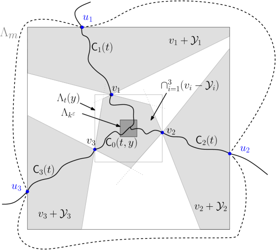
Figure 6: Description of the event $S(t,y)$, namely the cones and the decomposition of the cluster ${\sf C}$ into ${\sf C}_{i}(t)$ and $v_{i}(t)$, $i=1,2,3$.

Lemma 5.3.

Fix $\varepsilon_{1}>0$ and let $\varepsilon>0$ be sufficiently small. There exists $C>0$ such that

$$\mu_{\mathcal{D}}^{\sf f}\Bigl{(}\bigcup_{t\leq Ck^{\varepsilon}}\bigcup_{y\in\Lambda_{\varepsilon_{1}k}(x)}\mathcal{S}(t,y)\Bigm{|}E(u_{1},u_{2},u_{3},x)\Bigr{)}\geq 1-O({\rm e}^{-k^{\varepsilon}}).$$ (28)

Proof of Lemma 5.3.

First of all, we notice that coarse-graining on the $k^{\varepsilon}$-scale enables a reduction to particularly simple geometric structures. Consider a forest skeleton of the cluster ${\sf C}$ at scale $k^{\varepsilon}$. Note that, conditionally on $E(u_{1},u_{2},u_{3},x)$, this forest is in fact a tree $\mathcal{T}_{k^{\varepsilon}}$.

We define the trunk $\mathfrak{t}_{\varepsilon}$ of $\mathcal{T}_{k^{\varepsilon}}$ as the minimal subtree of $\mathcal{T}_{k^{\varepsilon}}$ which spans $\left\{u_{1},u_{2},u_{3}\right\}$.

We define the branches of $\mathcal{T}_{k^{\varepsilon}}$ as $\mathfrak{B}_{\varepsilon}=\mathcal{T}_{k^{\varepsilon}}\backslash\mathfrak{t}_{\varepsilon}$. In this case, we obtain the following reduced geometry of typical $\mathcal{T}_{k^{\varepsilon}}$, which holds uniformly in all situations in question, up to probabilities which are exponentially small in $k^{\varepsilon}$:

• $\mathcal{T}_{k^{\varepsilon}}$ does not have branches. This means that the tree $\mathcal{T}_{k^{\varepsilon}}$ consists only of a trunk which is a tripod, i.e. with one vertex of degree 3 and all other vertices of degree at most 2. We will write $x_{\varepsilon}$ for the only triple point of $\mathcal{T}_{k^{\varepsilon}}$, and $\mathcal{T}_{k^{\varepsilon}}^{i}=\{u_{i,\varepsilon}^{n_{i}},\dots,u_{i,\varepsilon}^{1}=x_{\varepsilon}\}$, $i=1,2,3$, for the three legs of $\mathcal{T}_{k^{\varepsilon}}$. Note that $u_{i}\in\hat{\mathbf{B}}_{2k^{\varepsilon}}(u_{i,\varepsilon}^{n_{i}})$.

• Fix $\kappa>0$ small. For every $\varepsilon>0$ and each ${\varepsilon^{\prime}}\in(0,\varepsilon/2)$, the skeletons $\mathcal{T}_{k^{\varepsilon^{\prime}}}^{i}\setminus\Lambda_{k^{\varepsilon}}(x_{\varepsilon^{\prime}})\subseteq x_{\varepsilon^{\prime}}+\mathcal{Y}_{i,2\kappa}$ as soon as $k$ becomes sufficiently large, where cones $\mathcal{Y}_{i,2\kappa}$ are defined via

  $$\mathcal{Y}_{i,r}=\bigl{\{}z:\measuredangle(z,u_{i}-x_{\varepsilon^{\prime}})\leq r\bigr{\}}.$$ (29)

  That is, the vertices of each of the three branches of $\mathcal{T}_{k^{\varepsilon^{\prime}}}$ outside the box $\Lambda_{k^{\varepsilon}}$ are confined to the respective cones $x_{\varepsilon^{\prime}}+\mathcal{Y}_{i,2\kappa}$.

Before proving Properties T1 and T2, let us describe how they can be used to prove the lemma. First of all, note that, by Proposition 4.6, we may assume that $|x_{\varepsilon^{\prime}}-x|\leq\delta_{1}k$ with $\delta_{1}>0$ fixed as small as we wish. In particular, we may assume that $u_{i}\in{\rm int}(x_{\varepsilon^{\prime}}+\mathcal{Y}_{i})$ (see Definition 5.1) and, consequently, that $\mathcal{Y}_{i,2\kappa}\subset\mathcal{Y}_{i}$.
By Proposition 4.5, the connected cluster ${\sf C}$ is included in $\mathcal{T}_{k^{\varepsilon^{\prime}}}+2k^{\varepsilon^{\prime}}{\bf U}_{\tau}$. Therefore, Properties T1 and T2 imply that ${\sf C}\setminus\Lambda_{k^{\varepsilon}}(x_{\varepsilon^{\prime}})=\tilde{\sf C}_{1}\cup\tilde{\sf C}_{2}\cup\tilde{\sf C}_{3}$, where $\tilde{\sf C}_{1}$, $\tilde{\sf C}_{2}$ and $\tilde{\sf C}_{3}$ are the clusters (in ${\sf C}\setminus\Lambda_{k^{\varepsilon}}(x_{\varepsilon^{\prime}})$) of $u_{1}$, $u_{2}$ and $u_{3}$ respectively. Note that, by T2, clusters ${\sf C}_{i}$ are confined to the sets (actually truncated cones) $(x_{\varepsilon^{\prime}}+\mathcal{Y}_{i,2\kappa}+2k^{\varepsilon^{\prime}}{\bf U}_{\tau})\setminus\Lambda_{k^{\varepsilon}}(x_{\varepsilon^{\prime}})$, which are well separated on the $k^{\varepsilon}$-scale. Consequently coarse-graining estimates developed in [10, Section 2] apply to each of ${\sf C}_{i}$ separately. As a result, the claim of Lemma 5.3 follows by a straightforward adaptation of the mass-gap arguments of [10, Section 2] applied separately to each of the three disjoint clusters $\tilde{\sf C}_{1},\tilde{\sf C}_{2}$ and $\tilde{\sf C}_{3}$. For instance, one can show the following: Fix $r$ large enough so that $\Lambda_{k^{\varepsilon^{\prime}}}(x_{\varepsilon^{\prime}})\subset v-\mathcal{Y}_{i}$ for any $v\in(x_{\varepsilon^{\prime}}+\mathcal{Y}_{i,2\kappa})\cap(\Lambda_{2rk^{\varepsilon}}(x_{\varepsilon^{\prime}})\setminus\Lambda_{rk^{\varepsilon}}(x_{\varepsilon^{\prime}}))$ and $i=1,2,3$. Then, up to probabilities which are exponentially small in $k^{\varepsilon}$, there exists $t\in[rk^{\varepsilon},2rk^{\varepsilon}]$ such that each of the clusters $\tilde{\sf C}_{i}$ contains a $\mathcal{Y}_{i}$-break point on $\partial\Lambda_{t}(x_{\varepsilon^{\prime}})$. That is,

• for $i=1,2,3$, the intersection $v_{i}=\tilde{\sf C}_{i}\cap\partial\Lambda_{t}(x_{\varepsilon})$ is a singleton;

• for $i=1,2,3$ the cluster $\tilde{\sf C}_{i}\subset(v_{i}+\mathcal{Y}_{i})\cup(v_{i}-\mathcal{Y}_{i})$.

This ensures $\mathcal{S}(t,y)$ for some $y\in\Lambda_{\varepsilon_{1}k}$ and (28) follows. ∎

For the proof of Property T1, we refer to [10, Lemma 2.1 and 2.2].

Proof of Property T2..

Let us start with a lower bound on $\mu_{\mathcal{D}}^{\sf f}(E(u_{1},u_{2},u_{3},x))$ which will be used later as a test threshold quantity for ruling out improbable events. Let $y$ be a lattice approximation of $x$. By the FKG inequality,

$$\mu_{\mathcal{D}}^{\sf f}(E(u_{1},u_{2},u_{3},x))\geq\mu_{\mathcal{D}}^{\sf f}\Bigl{(}\bigcap_{i=1}^{3}\bigl{\{}y\stackrel{{\scriptstyle\mathcal{D}}}{{\leftrightarrow}}u_{i}\bigr{\}}\Bigr{)}\geq\prod_{i=1}^{3}\mu_{\mathcal{D}}^{\sf f}\bigl{(}y\stackrel{{\scriptstyle\mathcal{D}}}{{\leftrightarrow}}u_{i}\bigr{)}.$$

Theorem A in [10] gives sharp asymptotics of quantities $\mu^{\sf f}\left(y\leftrightarrow v_{i}\right)$. These sharp asymptotics are built upon an effective random walk representation of events $\left\{y\leftrightarrow u\right\}$ as described in Subsection 4.1 of the the paper. Steps of this random walk have effective drift from $u_{i}$ towards $y$, and, since $\Lambda_{k}\subset\mathcal{D}$, it is easy to adjust the arguments therein in order to show that

$$\mu^{\sf f}_{\mathcal{D}}\bigl{(}y\stackrel{{\scriptstyle\mathcal{D}}}{{\leftrightarrow}}u\bigr{)}\geq\frac{C_{0}}{\sqrt{k}}{\rm e}^{-\tau(u-y)},$$

uniformly in $y\in\Lambda_{\frac{k}{2}}$ and $v\in\partial\Lambda_{k}$, where $C_{0}$ (and, similarly, $C_{1}$, $C_{2}$, $\ldots$ below) is a universal constant, in the sense that (30) applies uniformly in all the situations in question as soon as $k$ is sufficiently large. Consequently,

$$\mu_{\mathcal{D}}^{\sf f}(E(u_{1},u_{2},u_{3},x))\geq\exp\Bigl{(}-\sum_{i=1}^{3}\tau(u_{i}-x)-C_{1}\log k\Bigr{)},$$ (30)

also uniformly in all the situations in question as soon as $k$ is sufficiently large.

Next, let us say that ${\sf w}\in\mathcal{T}_{k^{\varepsilon^{\prime}}}^{i}$ is a $2\kappa$-cone point of $\mathcal{T}_{k^{\varepsilon^{\prime}}}^{i}$ if $\mathcal{T}_{k^{\varepsilon^{\prime}}}^{i}\subset\left(w-\mathcal{Y}_{i,2\kappa}\right)\cup\left(w+\mathcal{Y}_{i,2\kappa}\right)$. In our notation,

$$\tau(\mathcal{T}_{k^{\varepsilon^{\prime}}})=\sum_{i=1}^{3}\tau(\mathcal{T}_{k^{\varepsilon^{\prime}}}^{i})$$

Since $\tau$ is a strictly convex norm ([10, Subsection 1.3.2]) ,

$$\tau(\mathcal{T}_{k^{\varepsilon^{\prime}}}^{i})\geq\tau(u_{i}-x_{\varepsilon^{\prime}})\left(1+\delta(\kappa)\right)\geq\tau(u_{i}-x_{\varepsilon^{\prime}})+C_{2}k,$$ (31)

whenever $\mathcal{T}_{k^{\varepsilon^{\prime}}}^{i}$ does not contain $2\kappa$-cone points at all. This is essentially Lemma 2.4 of [10]. In view of (4.3), and in view of the lower bound (30), we are entitled to ignore the situation when any of the $\mathcal{T}_{k^{\varepsilon^{\prime}}}^{i}$ does not have $2\kappa$-cone points at all.

In the sequel, we use ${\sf w}^{*}_{i}$ to denote the first $2\kappa$-cone point of $\mathcal{T}_{k^{\varepsilon^{\prime}}}^{i}$ (starting at $x_{\varepsilon^{\prime}}$) and $N_{i}$ to denote its serial number; that is, ${\sf w}_{i}^{*}=u^{N_{i}}_{i,{\varepsilon^{\prime}}}$. Define $\mathcal{T}_{k^{\varepsilon^{\prime}}}^{i,*}=\{u^{1}_{i,{\varepsilon^{\prime}}},\ldots,u^{N_{i}}_{i,{\varepsilon^{\prime}}}={\sf w}_{i}^{*}\}$ as the portion of $\mathcal{T}_{k^{\varepsilon^{\prime}}}^{i}$ up to ${\sf w}_{i}^{*}$. Given $y$ and $\underline{{\sf w}}=\left({\sf w}_{1},{\sf w}_{2},{\sf w}_{3}\right)$, define the percolation event $E_{\varepsilon^{\prime}}(y,\underline{{\sf w}})\subset E(u_{1},u_{2},u_{3},x)$ as

$$E_{\varepsilon^{\prime}}(y,\underline{{\sf w}})=\bigl{\{}x_{\varepsilon^{\prime}}=y\,;\,{\sf w}_{i}^{*}={\sf w}_{i}\ \text{for $i=1,2,3$}\bigr{\}}.$$

In view of (30), Property T2 will follow as soon as we shall have checked that

$$\mu^{\sf f}_{\mathcal{D}}\left(E_{\varepsilon^{\prime}}(y,\underline{{\sf w}})\right)\leq{\rm e}^{-\sum_{i}\tau(u_{i}-y)-C_{3}k^{\varepsilon}},$$ (32)

uniformly in $k$, tripods $\mathcal{T}_{x}$, $y$ and $\underline{{\sf w}}\not\subset\Lambda_{k^{\varepsilon}}(y)$. For fixed realizations $\mathcal{T}^{i,*}$ of $\mathcal{T}^{i,*}_{k^{\varepsilon^{\prime}}}$ we have

$$\mu^{\sf f}_{\mathcal{D}}\bigl{(}E_{\varepsilon^{\prime}}(y,\underline{{\sf w}});\mathcal{T}^{i,*}_{k^{\varepsilon^{\prime}}}=\mathcal{T}^{i,*}\ \text{for $i=1,2,3$}\bigr{)}\leq{\rm exp}\Bigl{\{}-\sum_{i=1}^{3}\bigl{\{}\tau(u_{i}-{\sf w}_{i})+\tau(\mathcal{T}^{i,*})(1-{\mathrm{o}}_{k^{\varepsilon^{\prime}}}(1))\bigr{\}}+C_{4}k^{2{\varepsilon^{\prime}}}\Bigr{\}}.$$

This follows from (4.3) and from the finite energy property (applied for configurations on $\Lambda_{C_{5}k^{\varepsilon^{\prime}}}({\sf w}_{i})$) of the FK measures. Indeed, the finite energy property and the exponential ratio mixing property (6) enable to decouple between the event $\bigcap_{i}\bigl{\{}\mathcal{T}^{i,*}_{k^{\varepsilon^{\prime}}}=\mathcal{T}^{i,*}\bigr{\}}$ and the events $\bigcap_{i}\bigl{\{}{\sf w}_{i}\stackrel{{\scriptstyle{\sf w}_{i}+\mathcal{Y}_{i,2\kappa}}}{{\longleftrightarrow}}u_{i}\bigr{\}}$.

Assume, for instance, that ${\sf w}_{1}\not\in\Lambda_{k^{\varepsilon}}(y)$. There are two cases to consider:

Case 1: ${\sf w}_{1}\in y+\mathcal{Y}_{1,\kappa}$. Then, exactly as in (31), $\tau(\mathcal{T}^{1,*})\geq\tau({\sf w}_{1}-y)+C_{6}\left|{\sf w}_{1}-y\right|$. As in (21) the entropic factor related to the number of possible compatible realizations $\mathcal{T}^{1,*}$ is suppressed, and (32) follows as soon as we choose $\varepsilon>2{\varepsilon^{\prime}}$.

Case 2: ${\sf w}_{1}\in(y+\mathcal{Y}_{1,2\kappa})\backslash(y+\mathcal{Y}_{1,\kappa})$. By construction, $\tau(\mathcal{T}^{1,*})\geq\tau({\sf w}_{1}-y)$. However, by the sharp triangle inequality (2),

$$\tau({\sf w}_{1}-y)+\tau(u_{1}-{\sf w}_{1})-\tau(u_{1}-y)\geq C_{7}\left|{\sf w}_{1}-y\right|,$$

uniformly in ${\sf w}_{1}$ under consideration. Again, since the entropic factor is suppressed, (32) follows. ∎

Lemma 5.4.

Let $S_{\varepsilon}(y)=\bigcup_{t\leq Ck^{\varepsilon}}S(t,y)$. There exist two universal constants $\kappa>0$ and $C<\infty$ such that

$$\mu_{\mathcal{D}}^{\sf f}\bigl{(}S_{\varepsilon}(y)\bigm{|}E(u_{1},u_{2},u_{3},x)\bigr{)}=O\Bigl{(}k^{12\varepsilon-1}\exp\bigl{(}-\kappa\frac{\left|y-x\right|^{2}}{k}\bigr{)}\Bigr{)},$$ (33)

uniformly in $y\in\Lambda_{\varepsilon_{1}k}(x)$.

Proof.

Decompose

$$\mathcal{S}(t,y)=\bigcup_{W}\mathcal{S}^{W}(t,y)$$

according to the triple $W=\{v_{1}-y,v_{2}-y,v_{3}-y\}\subset\partial\Lambda_{t}$ which shows up in the definition. From now on, we set $w_{1}=v_{1}-y$, $w_{2}=v_{2}-y$ and $w_{3}=v_{3}-y$.

Since, under the event $S^{W}(t,y)$, we have that ${\sf C}_{0}\subseteq\bigcap_{i=1}^{3}\left(v_{i}-\mathcal{Y}_{i}\right)$ and that the points $u_{i}$ lie deep in the interior of the corresponding cones $v_{i}+\mathcal{Y}_{i}$, with $v_{i}\in\partial\Lambda_{t}(y)$ and $t\leq Ck^{\varepsilon}$, the Ornstein-Zernike asymptotics of [10, Theorem A] imply that

$$\mu_{\mathcal{D}}^{\sf f}\Bigl{(}\bigcap_{i=1}^{3}\{{\sf C}_{i}\subset v_{i}+\mathcal{Y}_{i}\}\Bigm{|}{\sf C}_{0}(t,y)\Bigr{)}=\Theta\bigl{(}k^{-3/2}\,{\rm e}^{-\sum_{i=1}^{3}\tau(u_{i}-v_{i})}\bigr{)},$$ (34)

uniformly in any possible realization ${\sf C}_{0}$ of ${\sf C}_{0}(t,y)$ compatible with $S^{W}(t,y)$. Note that if ${\sf C}_{0}(t,y)$ is compatible with $S^{W}(t,y)$, then shifts ${\sf C}_{0}^{u}\stackrel{{\scriptstyle\Delta}}{{=}}{\sf C}_{0}+u$ are compatible with shifted events $S^{W}(t,y+u)$.

Recall Definition 4.7 of $\phi(y)$. Given a triple $W=\left\{w_{1},w_{2},w_{3}\right\}\subset\Lambda_{Ck^{\varepsilon}}$, let us define

$$\phi_{W}(y)=\sum_{i=1}^{3}\tau(u_{i}-w_{i}-y).$$

Together with (34), we obtain

$$\frac{\mu_{\mathcal{D}}^{\sf f}\bigl{(}\mathcal{S}^{W}(t,y)\bigr{)}}{\mu_{\mathcal{D}}^{\sf f}\bigl{(}\mathcal{S}^{W}(t,z)\bigr{)}} =\frac{\sum_{{\sf C}_{0}}\mu_{\mathcal{D}}^{\sf f}\Bigl{(}\bigcap_{i=1}^{3}\{{\sf C}_{i}\subset y+w_{i}+\mathcal{Y}_{i}\}\Bigm{|}{\sf C}_{0}\Bigr{)}\mu_{\mathcal{D}}^{\sf f}({\sf C}_{0}(t,y)={\sf C}_{0})}{\sum_{{\sf C}_{0}}\mu_{\mathcal{D}}^{\sf f}\Bigl{(}\bigcap_{i=1}^{3}\{{\sf C}_{i}\subset z+w_{i}+\mathcal{Y}_{i}\}\Bigm{|}{\sf C}_{0}\Bigr{)}\mu_{\mathcal{D}}^{\sf f}({\sf C}_{0}(t,z)={\sf C}_{0}^{{z-y}})}$$

$$=\Theta\bigl{(}{\rm e}^{\phi_{W}(y)-\phi_{W}(z)}\bigr{)},$$ (35)

uniformly in $t\leq Ck^{\varepsilon}$, $W=\left\{w_{1},w_{2},w_{3}\right\}\subset\partial\Lambda_{t}$ and $y,z\in\Lambda_{\varepsilon_{1}k}$, where the sum is over ${\sf C}_{0}$ compatible with $S^{W}(t,y)$ and where in the last line we used classical ratio-mixing properties of subcritical random-cluster measures [3, Theorem 3.4] and (6) to compare $\mu_{\mathcal{D}}^{\sf f}({\sf C}_{0}(t,y)={\sf C}_{0})$ and $\mu_{\mathcal{D}}^{\sf f}({\sf C}_{0}(t,z)={\sf C}_{0}^{z-y})$.

The function $\phi_{W}$ has a non-degenerate quadratic minimum at some $x_{\rm min}(W)$ (see [9, Lemma 3]). In view of the homogeneity of $\tau$, a quadratic expansion around $x_{\rm min}$ yields

$$\phi_{W}(y)-\phi_{W}(x_{\rm min})=\Theta\Bigl{(}\frac{\left|y-x_{\rm min}\right|^{2}}{k}\Bigr{)},$$ (36)

uniformly in all situations in question. Since $|\phi(y)-\phi_{W}(y)|=O(k^{\varepsilon})$, its minimizers $x_{\rm min}(W)$ solve

$$F(x,W)\stackrel{{\scriptstyle\Delta}}{{=}}\nabla_{x}\phi_{W}(x)=0.$$

Since ${\rm Hess}(\phi)$ is non-degenerate at $x$, the implicit function theorem applies. As a result, $|x_{\rm min}(W)-x|=O(\sum_{i}\left|w_{i}\right|)=O(k^{\varepsilon})$ uniformly in all $W$ in question. This fact, together with (36), yields

$$\phi_{W}(y)-{\phi_{W}(x)}=\Theta\Bigl{(}\frac{\left|y-x\right|^{2}}{k}+k^{2\varepsilon-1}\Bigr{)}.$$ (37)

Since there are at most $O(k^{3\varepsilon})$ possible choices for $W$ and $O(k^{\varepsilon})$ possible choices for $t$, we deduce from (5) and (37) that

$$\frac{1}{O(k^{4\varepsilon})}\exp\bigl{(}-{C_{1}}\frac{|y-x|^{2}}{k}\bigr{)}\leq\frac{\mu_{\mathcal{D}}^{\sf f}(\mathcal{S}_{\varepsilon}(y))}{\mu_{\mathcal{D}}^{\sf f}(\mathcal{S}_{\varepsilon}({x}))}\leq O(k^{4\varepsilon})\exp\bigl{(}-{C_{2}}\frac{|y-x|^{2}}{k}\bigr{)}.$$ (38)

Above $\mathcal{S}_{\varepsilon}({x})$ means in fact $\mathcal{S}_{\varepsilon}(\lfloor x\rfloor)$. We can now compute

$$\mu_{\mathcal{D}}^{\sf f}(S_{\varepsilon}(y)\,|\,E(u_{1},u_{2},u_{3},x)) =\frac{\mu_{\mathcal{D}}^{\sf f}(S_{\varepsilon}(y))}{\mu_{\mathcal{D}}^{\sf f}(S_{\varepsilon}(x))}\cdot\frac{\mu_{\mathcal{D}}^{\sf f}(S_{\varepsilon}(x))}{\mu_{\mathcal{D}}^{\sf f}(E(u_{1},u_{2},u_{3},x))}$$

$$\leq O(k^{4\varepsilon})\exp\Bigl{(}-C_{2}\frac{|y-x|^{2}}{k}\Bigr{)}\frac{\mu_{\mathcal{D}}^{\sf f}(S_{\varepsilon}(x))}{\mu_{\mathcal{D}}^{\sf f}(E(u_{1},u_{2},u_{3},x))}$$ (39)

where we used the second inequality in (38). In order to see that the rightmost term in (5) is of the right order, observe that $|y-x|\leq k^{1/2-\varepsilon}$ implies that ${\rm e}^{-C_{2}|y-x|^{2}/k}$ is of order 1, and therefore the ratio in (38) is smaller than $O(k^{4\varepsilon})$. Therefore, by looking at the $k^{1-2\varepsilon}$ sites which are at distance at most $k^{1/2-\varepsilon}$ from $x$, we deduce, using the first inequality in (38), that

$$\mu_{\mathcal{D}}^{\sf f}(S_{\varepsilon}(x))\leq O(k^{-1+6\varepsilon})\sum_{y\in\Lambda_{k^{1/2-\varepsilon}}(x)}\mu_{\mathcal{D}}^{\sf f}(S_{\varepsilon}(y))\leq O(k^{-1+8\varepsilon})\mu_{\mathcal{D}}^{\sf f}(E(u_{1},u_{2},u_{3},x)),$$

where in the second inequality, we used the fact that in a given configuration there are at most $O(k^{2\varepsilon})$ sites $y$ such that the corresponding events $\mathcal{S}_{\varepsilon}(y)$ occur. This implies that

$$\frac{\mu_{\mathcal{D}}^{\sf f}\bigl{(}\mathcal{S}_{\varepsilon}(x)\bigr{)}}{\mu^{\sf f}_{\mathcal{D}}\bigl{(}E(u_{1},u_{2},u_{3},x)\bigr{)}}\leq O(k^{8\varepsilon-1}).$$

Together with (5), we obtain (33). ∎

Lemmas 5.3 and 5.4 imply that

$$\mu_{\mathcal{D}}^{\sf f}\bigl{(}{\sf C}\cap\Lambda_{k^{\varepsilon}}\neq\varnothing\bigm{|}E(u_{1},u_{2},u_{3},x)\bigr{)}\leq\\ O(k^{12\varepsilon-1})\sum_{y\in\Lambda_{\varepsilon_{1}k}(x)}{\rm e}^{-\kappa\left|y-x\right|^{2}/k}\mu_{\mathcal{D}}^{\sf f}\bigl{(}{\sf C}\cap\Lambda_{k^{\varepsilon}}\neq\varnothing\bigm{|}\mathcal{S}_{\varepsilon}(y)\bigr{)}+O\bigl{(}{\rm e}^{-k^{\varepsilon}}\bigr{)}.$$ (40)

It remains to provide an upper bound on $\mu_{\mathcal{D}}^{\sf f}\bigl{(}{\sf C}\cap\Lambda_{k^{\varepsilon}}\neq\varnothing\bigm{|}\mathcal{S}_{\varepsilon}(y)\bigr{)}$. There are two cases to consider:

Case 1: $y\in\Lambda_{2Ck^{\varepsilon}}$. In this case, we simply use

$$\mu_{\mathcal{D}}^{\sf f}\bigl{(}{\sf C}\cap\Lambda_{k^{\varepsilon}}\neq\varnothing\bigm{|}\mathcal{S}_{\varepsilon}(y)\bigr{)}\leq 1.$$ (41)

The total contribution to the right-hand side of (40) is then bounded by $O(k^{14\varepsilon-1})$, which is negligible with respect to our target estimate (27).

Case 2: $y\not\in\Lambda_{2Ck^{\varepsilon}}$. In this case, $\Lambda_{k^{\varepsilon}}$ can intersect at most one of the $\Lambda_{Ck^{\varepsilon}}(y)+\mathcal{Y}_{i}$, and therefore can be hit by only one cluster ${\sf C}_{i}$. Without loss of generality, let us assume that ${\sf C}_{i}={\sf C}_{1}$. Conditioning on the smallest $t$ such that $\mathcal{S}(t,y)$ occurs as well as on ${\sf C}_{0}$, ${\sf C}_{2}$ and ${\sf C}_{3}$, the cluster ${\sf C}_{1}$ obeys, as was explained after (25), a diffusive scaling. In particular,

$$\mu_{\mathcal{D}}^{\sf f}\bigl{(}z\in{\sf C}_{1}\bigm{|}S(t,y),{\sf C}_{0},{\sf C}_{2},{\sf C}_{3}\bigr{)}=O\Bigl{(}\frac{1}{\sqrt{|v_{1}-z|}}\,\exp\Bigl{[}-\kappa^{\prime}\frac{{\rm d}_{\tau}(z,[v_{1},u_{1}])^{2}}{\left|v_{1}-z\right|}\Bigr{]}\Bigr{)}.$$

In the previous inequality, $v_{1}=v_{1}(t,y)$. We find:

$$\mu_{\mathcal{D}}^{\sf f}\bigl{(}{\sf C}\cap\Lambda_{k^{\varepsilon}}\neq\varnothing\bigm{|}S(t,y),{\sf C}_{0},{\sf C}_{2},{\sf C}_{3}\bigr{)} \leq\sum_{z\in\partial\Lambda_{k^{\varepsilon}}}\mu_{\mathcal{D}}^{\sf f}\bigl{(}z\in{\sf C}_{1}\bigm{|}S(t,y),{\sf C}_{0},{\sf C}_{2},{\sf C}_{3}\bigr{)}$$

$$\leq\sum_{z\in\partial\Lambda_{k^{\varepsilon}}}O\Bigl{(}\frac{1}{\sqrt{|v_{1}-z|}}\,\exp\Bigl{[}-\kappa^{\prime}\frac{{\rm d}_{\tau}(z,[v_{1},u_{1}])^{2}}{\left|v_{1}-z\right|}\Bigr{]}\Bigr{)}$$

$$=O\Bigl{(}\frac{k^{\varepsilon}}{\sqrt{\left|y\right|}}\,\exp\bigl{\{}-\kappa^{\prime\prime}\frac{{\rm d}_{\tau}(0,[y,u_{1}])^{2}}{\left|y\right|}\bigr{\}}\Bigr{)}.$$ (42)

In the last line, we used the fact that $y,v_{1}\notin\Lambda_{Ck^{\varepsilon}}$ and $|v_{1}-y|\leq Ck^{\varepsilon}$. Let us substitute (42) into the sum on the right-hand side of (40) to obtain

$$\mu_{\mathcal{D}}^{\sf f}\bigl{(}{\sf C}\cap\Lambda_{k^{\varepsilon}}\neq\varnothing\bigm{|}E(u_{1},u_{2},u_{3},x)\bigr{)}\leq O({\rm e}^{-k^{\varepsilon}})+O(k^{14\varepsilon-1})\\ +O(k^{13\varepsilon-1})\sum_{y\in\Lambda_{\varepsilon_{1}k}(x)\setminus\Lambda_{2Ck^{\varepsilon}}}\frac{1}{\sqrt{|y|}}\exp\Big{[}-\kappa\frac{\left|y-x\right|^{2}}{k}-\kappa^{\prime\prime}\frac{{\rm d}_{\tau}(0,[y,u_{1}])^{2}}{|y|}\Big{]}.$$ (43)

After a simple estimate, one sees easily that the sum on the right is bounded above as

$$2\sum_{y\in\Lambda_{k^{1/2+\varepsilon}}(x)\setminus\Lambda_{2Ck^{\varepsilon}}}\frac{1}{\sqrt{|y|}}\exp\Big{[}-\kappa^{\prime\prime}\frac{{\rm d}_{\tau}(0,[y,u_{1}])^{2}}{|y|}\Big{]}\leq\sum_{\ell=\max\{2Ck^{\varepsilon},|x|-k^{1/2+\varepsilon}\}}^{|x|+k^{1/2+\varepsilon}}\frac{O(\sqrt{\ell})}{\sqrt{\ell}}=O(k^{\frac{1}{2}+\varepsilon}),$$

uniformly in $x$. In order to obtain the first inequality, we used the fact that $\exp(-\kappa|y-x|^{2}/k)$ is very small for sites outside of $\Lambda_{k^{1/2+\varepsilon}}(x)$. For the second, observe that sites $y$ at distance $\ell$ contributing substantially to this sum must satisfy the condition that $0$ is at distance $O(\sqrt{\ell})$ of $[y,u_{1}]$. There are $O(\sqrt{\ell})$ of them. This concludes the proof.

Acknowledgements.

H. D.-C. was supported by the EU Marie-Curie RTN CODY, the ERC AG CONFRA, as well as by the Swiss National Science Foundation. The research of D.I. was supported by the Israeli Science Foundation (grant No 817/09). L.C. and Y.V. were partially supported by the Swiss National Science Foundation.

References

• [1] M. Aizenman. Translation invariance and instability of phase coexistence in the two-dimensional Ising system. Comm. Math. Phys., 73(1):83–94, 1980.
• [2] M. Aizenman, J. T. Chayes, L. Chayes and C. M. Newman. Discontinuity of the magnetization in one-dimensional $1/|x-y|^{2}$ Ising and Potts models. J. Stat. Phys., 50(1): 1–40. 1988.
• [3] K. S. Alexander. On weak mixing in lattice models. Probab. Theory Relat. Fields, 110(4):441–471, 1998.
• [4] K. S. Alexander. Mixing properties and exponential decay for lattice systems in finite volumes Ann. Probab. 32(1A):441–487, 2004.
• [5] M. Alfaro, M. Conger, K. Hodges, A. Levy, R. Kochar, L. Kuklinski, Z. Mahmood and K. Von Haam. The structure of singularities in $\Phi$-minimizing networks in $\mathbb{R}^{2}$, Pacific J. of Math. 149(2):201–210, 1991.
• [6] V. Beffara and H. Duminil-Copin. The self-dual point of the two-dimensional random-cluster model is critical for $q\geq 1$. Probab. Theory Relat. Fields, 153(3), 511–542, 2012.
• [7] T. Bodineau. Translation invariant Gibbs states for the Ising model. Probab. Theory Relat. Fields, 135(2):153–168, 2006.
• [8] J. Bricmont, J. L. Lebowitz and C. E. Pfister. On the equivalence of boundary conditions. J. Statist. Phys., 21(5):573–582, 1979.
• [9] M. Campanino and M. Gianfelice. A local limit theorem for triple connections in subcritical Bernoulli percolation. Probab. Theory Relat. Fields, 143(3-4):353–378, 2009.
• [10] M. Campanino, D. Ioffe and Y. Velenik. Fluctuation theory of connectivities for subcritical random cluster models. Ann. Probab., 36(4):1287–1321, 2008.
• [11] J. T. Chayes, L. Chayes and R. H. Schonmann. Exponential decay of connectivities in the two-dimensional Ising model. J. Statist. Phys., 49(3-4):433–445, 1987.
• [12] E. J. Cockayne. On the Steiner problem, Canad. Math. Bull. 10:431–450, 1967.
• [13] L. Coquille and Y. Velenik. A finite-volume version of Aizenman–Higuchi theorem for the 2d Ising model. Probab. Theory Relat. Fields, 153(1-2):25–44, 2012.
• [14] O. Couronné. A large deviation result for the subcritical Bernoulli percolation. Annales de la Faculté des Sciences de Toulouse, 14(2), 201–2014, 2005.
• [15] R. L. Dobrushin and S. B. Shlosman. The problem of translation invariance of Gibbs states at low temperatures. In Mathematical physics reviews, Vol. 5, volume 5 of Soviet Sci. Rev. Sect. C Math. Phys. Rev., pages 53–195. Harwood Academic Publ., Chur, 1985.
• [16] R. L. Dobrušin. Gibbsian random fields for lattice systems with pairwise interactions. In Funkcional. Anal. i Priložen. 4(2):31–43, 1968.
• [17] R. L. Dobrušin. The Gibbs state that describes the coexistence of phases for a three-dimensional Ising model. Teor. Verojatnost. i Primenen., 17:619–639, 1972.
• [18] G. Gallavotti. The phase separation line in the two-dimensional Ising model. Comm. Math. Phys., 27:103–136, 1972.
• [19] H.-O. Georgii. Gibbs measures and phase transitions, volume 9 of de Gruyter Studies in Mathematics. Walter de Gruyter & Co., Berlin, 1988.
• [20] H.-O. Georgii, O. Häggström and C. Maes. The random geometry of equilibrium phases. In Phase transitions and critical phenomena, Phase Transit. Crit. Phenom., vol. 18, pp. 1–142, Academic Press, San Diego, 2001.
• [21] H.-O. Georgii and Y. Higuchi. Percolation and number of phases in the two-dimensional Ising model. J. Math. Phys., 41(3):1153–1169, 2000.
• [22] L. Greenberg and D. Ioffe. On an invariance principle for phase separation lines. Ann. Inst. H. Poincaré Probab. Statist., 41(5):871–885, 2005.
• [23] G. R. Grimmett. The random-cluster model, vol. 333 of Grundlehren der Mathematischen Wissenschaften, Springer-Verlag, Berlin, 2006.
• [24] Y. Higuchi. On some limit theorems related to the phase separation line in the two-dimensional Ising model. Z. Wahrsch. Verw. Gebiete, 50(3):287–315, 1979.
• [25] Y. Higuchi. On the absence of non-translation invariant Gibbs states for the two-dimensional Ising model. In Random fields, Vol. I, II (Esztergom, 1979), volume 27 of Colloq. Math. Soc. János Bolyai, pages 517–534. North-Holland, Amsterdam, 1981.
• [26] D. Ioffe. Large deviations for the 2D Ising model: a lower bound without cluster expansions. J. Statist. Phys., 74(1-2):411–432, 1994.
• [27] L. Laanait, A. Messager, S. Miracle-Solé, J. Ruiz and S. Shlosman. Interfaces in the Potts model. I. Pirogov-Sinai theory of the Fortuin-Kasteleyn representation. Comm. Math. Phys., 140(1):81–91, 1991.
• [28] L. Laanait, A. Messager and J. Ruiz. Phases coexistence and surface tensions for the Potts model. Comm. Math. Phys., 105(4):527–545, 1986.
• [29] O. E. Lanford and D. Ruelle. Observables at infinity and states with short range correlations in statistical mechanics. Comm. Math. Phys., 13:194–215, 1969.
• [30] D. H. Martirosian. Translation invariant Gibbs states in the $q$-state Potts model. Comm. Math. Phys., 105(2):281–290, 1986.
• [31] A. Messager and S. Miracle-Sole. Correlation functions and boundary conditions in the Ising ferromagnet. J. Statist. Phys., 17(4):245–262, 1977.
• [32] S. A. Pirogov and Ja. G. Sinaĭ. Phase diagrams of classical lattice systems. Teoret. Mat. Fiz., 25(3):358–369, 1975.
• [33] C-E. Pfister and Y. Velenik. Interface, Surface Tension and Reentrant Pinning Transition in the 2D Ising Model . Comm. Math. Phys. 204(2), 269–312, 1998.
• [34] L. Russo. The infinite cluster method in the two-dimensional Ising model. Comm. Math. Phys., 67(3):251–266, 1979.
• [35] M. Zahradník. An alternate version of Pirogov-Sinaĭ theory. Comm. Math. Phys., 93(4):559–581, 1984.
Département de Mathématiques
Université de Genève
Genève, Switzerland
E-mail: loren.coquille@unige.ch; hugo.duminil@unige.ch; yvan.velenik@unige.ch
Faculty of IE&M
Technion
Haifa, Israel
E-mail: ieioffe@ie.technion.ac.il