Abstract

Using the language of non-relativistic effective Lagrangians, we formulate a systematic framework for the calculation of resonance matrix elements in lattice QCD. The generalization of the Lüscher-Lellouch formula for these matrix elements is derived. We further discuss in detail the procedure of the analytic continuation of the resonance matrix elements into the complex energy plane and investigate the infinite-volume limit.

Pacs:	11.10.St, 11.15.Ha, 13.40.Gp
Keywords:	Resonances in lattice QCD, field theory in a finite volume,
	Non-relativistic effective field theory, Form factors

1 Introduction

The calculation of matrix elements involving unstable states has already been addressed in lattice QCD. As examples, we mention the recent papers [1, 2, 3], which deal with the electromagnetic form factor of the $\rho$-meson, as well as the electromagnetic and axial-vector form factors of the $\Delta$-resonance and the $N\Delta\gamma$ transition vertex. Electromagnetic and axial transition form factors for the Roper resonance have also been studied [4]. Moreover, we expect that the number of such investigations will substantially grow in the nearest future due to a growing interest in the study of the excited states.

Even if one argues that the quark (pion) masses in the above lattice simulations are large, so that all resonances are in fact stable particles, various conceptual questions arise:

• It is clear that we are ultimately interested in simulations carried out at the physical quark masses. Is it possible (at least in principle) to tune the quark mass continuously until it reaches the physical value?

• In the continuum field theory, any matrix element with resonance states is defined through an analytic continuation of the three-point Green function into the complex plane $P^{2}\to s_{R}$, where $P$ denotes the pertinent four-momentum and $s_{R}$ is the resonance pole position in the complex plane (its real and imaginary parts are related to the mass and the width of a resonance). What is the analog of this procedure in lattice field theory?

• Once this procedure is defined, what is the volume dependence of the measured form factors?

In this paper, we address these questions in detail. In order to formulate the problem in a more transparent manner, let us first define what is meant by resonance matrix elements in the continuum field theory and on the lattice. We start with the continuum field theory and, for simplicity, concentrate on the scalar case. Consider an arbitrary (local or non-local) scalar operator $O(x)$ which has the internal quantum numbers of a given resonance. The statement that a resonance is present is equivalent to the claim that the two-point function

$$D(P^{2})=i\int d^{4}x\,e^{iPx}\langle 0|TO(x)O^{\dagger}(0)|0\rangle$$ (1)

has a pole in the complex variable $P^{2}$ on the lower half of the second Riemann sheet at $P^{2}=s_{R}$:

$$\lim_{P^{2}\to s_{R}}D(P^{2})=\frac{B_{R}}{s_{R}-P^{2}}+\mbox{regular terms at }P^{2}\to s_{R}\,.$$ (2)

The real and imaginary parts of $s_{R}$ are related to the resonance mass $m_{R}$ and the width $\Gamma_{R}$, according to $\mbox{Re}\,s_{R}=m_{R}^{2}-\Gamma_{R}^{2}/4$, $\mbox{Im}\,s_{R}=-m_{R}\Gamma_{R}$.

In order to define resonance matrix elements, say, of the electromagnetic current $J_{\mu}$, we consider the following three-point function:

$$V_{\mu}(P,Q)=i^{2}\int d^{4}x\,d^{4}y\,e^{iPx-iQy}\langle 0|TO(x)J_{\mu}(0)O^{\dagger}(y)|0\rangle\,.$$ (3)

The form factor of a resonance is then defined as

$$i(P+Q)_{\mu}F((P-Q)^{2})\doteq\langle P|J_{\mu}(0)|Q\rangle=\lim_{P^{2},Q^{2}\to s_{R}}B_{R}^{-1/2}(s_{R}-P^{2})V_{\mu}(P,Q)(s_{R}-Q^{2})B_{R}^{-1/2}\,,$$ (4)

where $B_{R}$ is the residue at the resonance pole, see Eq. (2). Note that the matrix element displayed in Eq. (4) should be understood as a mere notation: in the spectrum, there exists no isolated resonance state with a definite momentum. Moreover, as it is clear from Eq. (4), this definition of the resonance matrix elements necessarily implies an analytic continuation into the complex plane. We would like to stress that we are not aware of any consistent field-theoretical prescription, where the analytic continuation would not be employed.

Let us now ask the question, how such resonance matrix elements could be evaluated on the lattice (at least, in principle). As it is well known, a resonance does not appear as an isolated energy level. There exist alternative approaches to the problem of extracting resonance characteristics (the mass and the width) from the measured quantities on the Euclidean lattice. In this paper, we work within Lüscher’s finite-volume framework [7]. In order to calculate the matrix element on the lattice, one usually considers the following three-point function

$$\tilde{V}_{\mu}({\bf P},t^{\prime};{\bf Q},t)=\langle 0|TO_{\bf P}(t^{\prime})J_{\mu}(0)O_{\bf Q}^{\dagger}(t)|0\rangle\,,$$ (5)

where

$$O_{\bf P}(t^{\prime})=\sum_{\bf x}e^{-i{\bf Px}}O({\bf x},t^{\prime})\,,\quad\quad O_{\bf Q}^{\dagger}(t)=\sum_{\bf y}e^{i{\bf Qy}}O^{\dagger}({\bf y},t)\,.$$ (6)

In addition, we define:

$$D({\bf P},t)=\langle 0|TO_{\bf P}(t)O^{\dagger}_{\bf P}(0)|0\rangle\,.$$ (7)

The matrix element of the electromagnetic current between the ground-state vectors in a channel with the quantum numbers of the operator $O(x)$, moving with the 3-momenta ${\bf P}$ and ${\bf Q}$, respectively, is given by

$$\langle E_{0}({\bf P})|J_{\mu}(0)|E_{0}({\bf Q})\rangle=\displaystyle\lim_{\begin{subarray}{c}t^{\prime}\to+\infty\\ t\to-\infty\end{subarray}}\tilde{V}_{\mu}({\bf P},t^{\prime};{\bf Q},t)\sqrt{\frac{D({\bf Q},t^{\prime})D({\bf P},t)}{D({\bf Q},t)D({\bf Q},t^{\prime}-t)D({\bf P},t-t^{\prime})D({\bf P},t^{\prime})}}.$$ (8)

Using the generalized eigenvalue equation method, the matrix elements between the excited state vectors $|E_{n}({\bf P})\rangle$ can be also defined in a similar manner.

If the ground state of a system corresponds to a stable particle, then Eq. (8) indeed yields the form factor of a stable particle in the infinite-volume limit, which in this case is well defined. However, the situation in case of resonances is conceptually different. The easiest way to see this is to note that in the infinite-volume limit the energy of any state $|E_{n}({\bf P})\rangle$ tends to the two-particle threshold energy. In other words, any given energy level decays into the free particle levels in the limit $L\to\infty$ (here, $L$ denotes the size of a spatial box). Moreover, as shown in Ref. [23] (in case of $1+1$ dimensions), the matrix elements measured for any given level follow a similar pattern. For example, the magnetic moment tends to the sum of the magnetic moments of the free particles in the limit $L\to\infty$. Obviously, this is not the result that we wish to extract from lattice data.

As mentioned above, using Lüscher’s approach, it is possible to determine the resonance pole position in the complex plane from the measured finite-volume (real) energy spectrum. This position stays put (up to exponentially suppressed corrections in $L$) in the limit $L\to\infty$, despite the fact that all individual levels collapse towards threshold in this limit. The aim of the present paper is to formulate a similar approach for the matrix elements, and to ensure that the matrix elements that are extracted with the help of such a procedure coincide with the infinite-volume matrix elements, e.g., given in Eq. (4), up to exponentially suppressed corrections.

The goal, stated above, will be achieved by a systematic use of non-relativistic effective field theory (EFT) in a finite volume. In particular, we shall calculate the quantity in Eq. (8), which can be measured on the lattice, within non-relativistic EFT, and shall identify a piece in this expression, whose infinite-volume limit coincides with the resonance matrix element in the infinite volume we are looking for.

The paper is organized as follows: In section 2 we formulate a covariant non-relativistic EFT in a moving frame and re-derive the Gottlieb-Rummukainen [24] formula within this approach. The extraction of a resonance pole position is discussed in detail. In section 3 we give a short re-derivation of the Lüscher-Lellouch formula [19], as another application of the non-relativistic EFT methods. Further, in section 4 we evaluate the vertex function in the non-relativistic EFT. The infinite-volume limit of different terms in the expression of the vertex function is analyzed in detail in section 5, where particular attention is paid to the so-called fixed singularities that emerge in a result of analytic continuation of Lüscher’s zeta-function into the complex plane in $3+1$ dimensions. The prescription for calculating the resonance matrix elements is given in section 6. Section 7 contains our conclusions.

2 Extraction of the resonance poles in moving frames

The initial and final states in a form factor have non-zero momenta. For this reason, one has to formulate a procedure for extracting resonance pole positions in moving frames. Within potential quantum mechanics, this has been done in Refs. [24], see also Ref. [25, 26] for the generalization to the non-equal mass case. Refs. [20, 27] address the same problem in a field-theoretical setting. Finally, in Ref. [28], a full group-theoretical analysis of the resulting equation has been performed, including the case of particles with spin. Below, we shall briefly re-derive this result within the non-relativistic EFT along the lines similar to Refs. [29, 30], where the treatment was restricted to the rest frame. At a later stage, the same approach will be used for the calculation of the matrix elements.

In the treatment of the moving frames it is very convenient to use the covariant form of the non-relativistic EFT which has been introduced in Ref. [31] and was discussed in detail in Ref. [32]. Assume, for simplicity, that we deal with two elementary scalar fields $\Phi_{1,2}$ with masses $m_{1,2}$, respectively. The Lagrangian is given in the following form:

$${\cal L} = \sum_{i=1,2}\Phi_{i}^{\dagger}2W_{i}(i\partial_{t}-W_{i})\Phi_{i}+C_{0}\Phi_{1}^{\dagger}\Phi_{1}\Phi_{2}^{\dagger}\Phi_{2}$$ (9)

$$+ C_{1}\bigl{(}(\Phi_{1}^{\dagger})^{\mu}(\Phi_{2}^{\dagger})_{\mu}\Phi_{1}\Phi_{2}-m_{1}m_{2}\Phi_{1}^{\dagger}\Phi_{1}\Phi_{2}^{\dagger}\Phi_{2}+\mbox{h.c.}\bigr{)}$$

$$+ C_{2}\bigl{(}\Phi_{1}^{\dagger}(\Phi_{2}^{\dagger})^{\mu}-(\Phi_{1}^{\dagger})^{\mu}\Phi_{2}^{\dagger})((\Phi_{1})_{\mu}\Phi_{2}-\Phi_{1}(\Phi_{2})_{\mu})+\cdots\,,$$

where $\Phi_{i},~{}i=1,2$ denote the non-relativistic field operators, $W_{i}=\sqrt{m_{i}^{2}+\triangle}$ are the energies of the particles (here, $\triangle\doteq\nabla^{2}$), and

$$(\Phi_{i})_{\mu}=({\cal P}_{i})_{\mu}\Phi_{i}\,,\quad(\Phi_{i}^{\dagger})_{\mu}=({\cal P}_{i}^{\dagger})_{\mu}\Phi_{i}^{\dagger}\,,\quad\quad({\cal P}_{i})_{\mu}=(W_{i},-i\nabla)\,,\quad({\cal P}_{i}^{\dagger})_{\mu}=(W_{i},i\nabla)\,.$$ (10)

Further, the ellipses stand for terms containing at least four space derivatives. To set up the power-counting rules we introduce, as in Refs. [31, 32], a generic small parameter $\epsilon$ and count each 3-momentum as ${\bf p}_{i}=O(\epsilon)$, whereas the masses are counted as $m_{i}=O(1)$. The Lagrangian given in Eq. (9) contains all allowed explicitly Lorentz-invariant terms up-to-and-including $O(\epsilon^{2})$, and the omitted terms are of order $\epsilon^{4}$.

The non-relativistic couplings $C_{0},C_{1},C_{2},\cdots$, which are present in the Lagrangian, are directly related to the effective-range expansion parameters for $1+2\to 1+2$ elastic scattering (scattering length, effective range, etc), see Refs. [31, 32]. We would like to remind the reader here that the theory described by the Lagrangian given in Eq. (9) conserves particle number, so it can be applied in the elastic region only.

The Feynman rules, which are produced by the Lagrangian (9), should be amended by a prescription which states that the integrand in each Feynman integral is expanded in 3-momenta, each term is integrated by using dimensional regularization and the result is summed up again [31, 32]. Below, we shall consider the theory in a finite volume. It is easy to see that, for consistency, one should apply the same prescription, replacing the dimensionally regularized integrals by sums over discrete momenta. In particular, one has to discard everywhere discrete sums over polynomials in momenta, in accordance with the similar infinite-volume prescription in the dimensionally regularized theory.

Let us start in the infinite volume. Using the above Feynman rules, it is straightforward to ensure that the scattering $T$-matrix in the infinite volume in an arbitrary moving frame obeys the Lippmann-Schwinger (LS) equation:

$$T({\bf p}_{1},{\bf p}_{2};{\bf q}_{1},{\bf q}_{2})=-V({\bf p}_{1},{\bf p}_{2};{\bf q}_{1},{\bf q}_{2})-\int\frac{d^{d}{\bf k}_{1}}{(2\pi)^{d}2w_{1}({\bf k}_{1})}\frac{d^{d}{\bf k}_{2}}{(2\pi)^{d}2w_{2}({\bf k}_{2})}\,$$ (11)

$$\times (2\pi)^{d}\delta^{d}({\bf p}_{1}+{\bf p}_{2}-{\bf k}_{1}-{\bf k}_{2})\,\frac{V({\bf p}_{1},{\bf p}_{2};{\bf k}_{1},{\bf k}_{2})T({\bf k}_{1},{\bf k}_{2};{\bf q}_{1},{\bf q}_{2})}{w_{1}({\bf k}_{1})+w_{2}({\bf k}_{2})-w_{1}({\bf p}_{1})-w_{2}({\bf p}_{2})-i0}\,,$$

where $w_{i}({\bf l})=\sqrt{m_{i}^{2}+{\bf l}^{2}}$ and the potential is given by the matrix element of the interaction Hamiltonian, which is derived from the Lagrangian (9) by the canonical procedure, between the two-particle states

$$\langle{\bf p}_{1},{\bf p}_{2}|H_{\rm I}|{\bf q}_{1},{\bf q}_{2}\rangle = (2\pi)^{3}\delta^{3}({\bf p}_{1}+{\bf p}_{2}-{\bf q}_{1}-{\bf q}_{2})V({\bf p}_{1},{\bf p}_{2};{\bf q}_{1},{\bf q}_{2})\,.$$ (12)

Note that we have used dimensional regularization in Eq. (11). The parameter $d$ denotes the number of space dimensions (at the end of calculations, $d\to 3$).

By construction, the potential $V$ is a Lorentz-invariant low-energy polynomial that depends only on scalar products of the 4-momenta. The first few terms in the expansion are given by

$$-V({\bf p}_{1},{\bf p}_{2};{\bf q}_{1},{\bf q}_{2})=C_{0}+C_{1}(p_{1}p_{2}+q_{1}q_{2}-2m_{1}m_{2})+C_{2}(p_{2}-p_{1})(q_{2}-q_{1})+O(\epsilon^{4})\,,$$ (13)

where, e.g., $p_{1}p_{2}=w_{1}({\bf p}_{1})w_{2}({\bf p}_{2})-{\bf p}_{1}{\bf p}_{2}$, etc. In general, defining the center-of-mass (CM) and relative momenta, according to

$$\!\!\!\!P=p_{1}+p_{2}\,,\quad p=\mu_{2}p_{1}-\mu_{1}p_{2}\,,\quad\quad\mu_{1,2}=\frac{1}{2}\biggl{(}1\pm\frac{m_{1}^{2}-m_{2}^{2}}{P^{2}}\biggr{)}\,,\quad p^{2}=\frac{\lambda(P^{2},m_{1}^{2},m_{2}^{2})}{4P^{2}}\,,$$

$$\!\!\!\!Q=q_{1}+q_{2}\,,\quad q=\mu_{2}^{\prime}q_{1}-\mu_{1}^{\prime}q_{2}\,,\quad\quad\mu^{\prime}_{1,2}=\frac{1}{2}\biggl{(}1\pm\frac{m_{1}^{2}-m_{2}^{2}}{Q^{2}}\biggr{)}\,,\quad q^{2}=\frac{\lambda(Q^{2},m_{1}^{2},m_{2}^{2})}{4Q^{2}}\,,$$ (14)

where $\lambda(x,y,z)$ denotes the Källén triangle function, it can be seen that $V$ is a low-energy polynomial of six independent Lorentz-invariant arguments $p^{2}$, $q^{2}$, $pq$, $PQ$, $Pq$, $pQ$. The original arguments $p_{1}p_{2}$, $p_{1}q_{1}$, $p_{1}q_{2}$, $p_{2}q_{1}$, $p_{2}q_{2}$, $q_{1}q_{2}$ can be expressed through linear combinations of these arguments with coefficients, which themselves are low-energy polynomials.

Consider now the partial-wave expansion of the potential. To this end, we define the momenta boosted to the CM frame (note that the boost velocity is different in the initial and the final states, because the potential is generally off the energy shell):

$${\bf p}^{*}={\bf p}+{\bf P}\biggl{(}(\gamma-1)\frac{{\bf p}{\bf P}}{{\bf P}^{2}}-\gamma v\frac{p_{0}}{|{\bf P}|}\biggr{)}\,,\quad p_{0}^{*}=\gamma p_{0}-\gamma v\frac{{\bf p}{\bf P}}{|{\bf P}|}=0\,,$$

$$P^{*}_{\mu}=(\sqrt{P^{2}},{\bf 0})\,,\quad\quad v=\frac{|{\bf P}|}{P_{0}}\,,\quad\gamma=(1-v^{2})^{-1/2}\,,$$

$${\bf q}^{*}={\bf q}+{\bf Q}\biggl{(}(\gamma^{\prime}-1)\frac{{\bf q}{\bf Q}}{{\bf Q}^{2}}-\gamma^{\prime}v^{\prime}\frac{q_{0}}{|{\bf Q}|}\biggr{)}\,,\quad q_{0}^{*}=\gamma^{\prime}q_{0}-\gamma^{\prime}v^{\prime}\frac{{\bf q}{\bf Q}}{|{\bf Q}|}=0\,,$$

$$Q^{*}_{\mu}=(\sqrt{Q^{2}},{\bf 0})\,,\quad\quad v^{\prime}=\frac{|{\bf Q}|}{Q_{0}}\,,\quad\gamma^{\prime}=(1-(v^{\prime})^{2})^{-1/2}\,.$$ (15)

Taking into account the fact that ${\bf P}={\bf Q}$ in the “lab frame,” it is straightforward to show that

$$pq = p^{*}q^{*}+O((P^{0}-Q^{0})^{2})=-{\bf p}^{*}{\bf q}^{*}+O((P^{0}-Q^{0})^{2})\,,$$

$$PQ = =P^{*}Q^{*}+O((P_{0}-Q_{0})^{2})=\sqrt{P^{2}}\sqrt{Q^{2}}+O((P_{0}-Q_{0})^{2})\,,$$

$$Pq = P^{*}q^{*}+O(P_{0}-Q_{0})=0+O(P_{0}-Q_{0})\,,$$

$$pQ = p^{*}Q^{*}+O(P_{0}-Q_{0})=0+O(P_{0}-Q_{0})\,.$$ (16)

In addition, $p^{2}$ and $q^{2}$ can be expressed in terms of $P^{2}$ and $Q^{2}$, respectively. This means that, up to terms that vanish as $P_{0}\to Q_{0}$, the potential can be rewritten in the following form

$$-V({\bf p}_{1},{\bf p}_{2};{\bf q}_{1},{\bf q}_{2})=-4\pi\sum_{lm}v_{l}(|{\bf p}^{*}|,|{\bf q}^{*}|){\cal Y}_{lm}({\bf p}^{*}){\cal Y}^{*}_{lm}({\bf q}^{*})+O(P_{0}-Q_{0})\,.$$ (17)

Here, the function $v_{l}$ can be chosen to be real and symmetric with respect to its arguments, i.e., Eq. (17) describes a Hermitean potential. The quantity ${\cal Y}_{lm}({\bf p})$ is defined as ${\cal Y}_{lm}({\bf p})=|{\bf p}|^{l}Y_{lm}(\hat{\bf p})$, where $Y_{lm}$ are the usual spherical harmonics. The terms that vanish as $P_{0}\to Q_{0}$ can be omitted from now on. The justification for this is the fact that the parameters in the potential are determined by matching to the physical $S$-matrix elements (on shell), order by order in the low-energy expansion. The omitted terms do not contribute either at tree level or in loops (the latter because the regular momentum integrals vanish in dimensional regularization). Consequently, one may consistently set these terms equal to zero from the beginning.

Performing now the partial-wave expansion in the amplitude

$$T({\bf p}_{1},{\bf p}_{2};{\bf q}_{1},{\bf q}_{2})=4\pi\sum_{lm}t_{l}(|{\bf p}^{*}|,|{\bf q}^{*}|){\cal Y}_{lm}({\bf p}^{*}){\cal Y}^{*}_{lm}({\bf q}^{*})\,,$$ (18)

substituting this expansion into the LS equation (11), and using the properties of dimensional regularization, on the energy shell $|{\bf p}^{*}|=|{\bf q}^{*}|=\lambda^{1/2}(s,m_{1}^{2},m_{2}^{2})/(2\sqrt{s})$ we get

$$t_{l}(s)=-v_{l}(s)-v_{l}(s)|{\bf p}^{*}|^{2l}G(s)t_{l}(s)\,,$$ (19)

where the obvious shorthand notations for the on-shell quantities $v_{l}(s)=v_{l}(|{\bf p}^{*}|,|{\bf p}^{*}|)$ and $t_{l}(s)=t_{l}(|{\bf p}^{*}|,|{\bf p}^{*}|)$ are used. The quantity $G(s)$ is given by [31, 32]:

$$G(s)=\int\frac{d^{d}{\bf k}_{1}}{(2\pi)^{d}2w_{1}({\bf k}_{1})}\frac{d^{d}{\bf k}_{2}}{(2\pi)^{d}2w_{2}({\bf k}_{2})}\,\frac{(2\pi)^{d}\delta^{d}({\bf P}-{\bf k}_{1}-{\bf k}_{2})}{w_{1}({\bf k}_{1})+w_{2}({\bf k}_{2})-P_{0}-i0}=\frac{i|{\bf p}^{*}|}{8\pi\sqrt{s}}\,.$$ (20)

Further, unitarity gives:

$$t_{l}(s)=\frac{8\pi\sqrt{s}}{|{\bf p}^{*}|^{2l+1}}\,e^{i\delta_{l}(s)}\sin\delta_{l}(s)\,,\quad\quad v_{l}(s)=-\frac{8\pi\sqrt{s}}{|{\bf p}^{*}|^{2l+1}}\,\tan\delta_{l}(s)\,,$$ (21)

where $\delta_{l}(s)$ is the scattering phase.

The transition to the finite volume is performed in the “lab frame”. The momenta are discretized according to

$${\bf k}_{i}=\frac{2\pi}{L}\,{\bf n}_{i}\,,\quad\quad{\bf n}_{i}\in\mathbb{Z}^{3}\,.$$ (22)

The partial-wave expansion of the potential does not change. However, since the introduction of a cubic box breaks rotational symmetry, the partial-wave expansion of the scattering amplitude has to be modified:

$$T({\bf p}_{1},{\bf p}_{2};{\bf q}_{1},{\bf q}_{2})=(4\pi)\sum_{lm,l^{\prime}m^{\prime}}t_{lm,l^{\prime}m^{\prime}}(|{\bf p}^{*}|,|{\bf q}^{*}|;{\bf P}){\cal Y}_{lm}({\bf p}^{*}){\cal Y}^{*}_{l^{\prime}m^{\prime}}({\bf q}^{*})\,.$$ (23)

Substituting this expression into the Lippmann-Schwinger equation, on the energy shell we obtain:

$$t_{lm,l^{\prime}m^{\prime}}(s;{\bf P})=-\delta_{lm,l^{\prime}m^{\prime}}v_{l}(s)-4\pi\sum_{l^{\prime\prime}m^{\prime\prime}}v_{l}(s){\cal X}_{lm,l^{\prime\prime}m^{\prime\prime}}(s,{\bf P})t_{l^{\prime\prime}m^{\prime\prime},l^{\prime}m^{\prime}}(s;{\bf P})\,,$$ (24)

where

$${\cal X}_{lm,l^{\prime}m^{\prime}}(s,{\bf P})=\frac{1}{L^{3}}\sum_{{\bf k}_{1}}\frac{{\cal Y}^{*}_{lm}({\bf k}^{*}){\cal Y}_{l^{\prime}m^{\prime}}({\bf k}^{*})}{2w_{1}({\bf k}_{1})2w_{2}({\bf P}-{\bf k}_{1})(w_{1}({\bf k}_{1})+w_{2}({\bf P}-{\bf k}_{1})-P_{0})}\,.$$ (25)

Next, we use the identity [32]

$$\frac{1}{4w_{1}w_{2}(w_{1}+w_{2}-P_{0})} = \frac{1}{2P_{0}}\frac{1}{{\bf k}^{2}-\dfrac{({\bf k}{\bf P})^{2}}{P_{0}^{2}}-({\bf p}^{*})^{2}}$$ (26)

$$+ \frac{1}{4w_{1}w_{2}}\biggl{(}\frac{1}{w_{1}+w_{2}+P_{0}}-\frac{1}{w_{1}-w_{2}+P_{0}}-\frac{1}{w_{2}-w_{1}+P_{0}}\biggr{)}\,,$$

where ${\bf k}={\bf k}_{1}+\mu_{1}{\bf P}$. One can straightforwardly check that the term in the brackets does not become singular in the physical region. Using the regular summation theorem [34], one may then replace the sum over ${\bf k}_{1}$ in this term by the integral. Further, to be consistent with our prescription for the calculation of the Feynman integrals in dimensional regularization, one should put these integrals to zero. After this, the expression for ${\cal X}_{lm,l^{\prime}m^{\prime}}(s,{\bf P})$ takes the following form:

$${\cal X}_{lm,l^{\prime}m^{\prime}}(s,{\bf P})=\frac{1}{2P_{0}}\,\frac{1}{L^{3}}\sum_{{\bf k}={\bf k}_{1}+\mu_{1}{\bf P}}\frac{{\cal Y}^{*}_{lm}({\bf k}^{*}){\cal Y}_{l^{\prime}m^{\prime}}({\bf k}^{*})}{{\bf k}^{2}-\dfrac{({\bf k}{\bf P})^{2}}{P_{0}^{2}}-({\bf p}^{*})^{2}}\,.$$ (27)

In order to transform this equation further, let us define the parallel and perpendicular components of the three vectors with respect to the CM momentum ${\bf P}$. In particular, one may write ${\bf k}^{*}=(k^{*}_{\parallel},{\bf k}^{*}_{\perp})$, where $k^{*}_{\parallel}=(\gamma^{*})^{-1}k_{\parallel}$, ${\bf k}^{*}_{\perp}={\bf k}_{\perp}$ and $\gamma^{*}=(1-(v^{*})^{2})^{-1/2}$, $v^{*}=|{\bf P}|/E^{*}=|{\bf P}|/(w_{1}({\bf k}^{*})+w_{2}({\bf k}^{*}))$. Consequently, on the energy shell $E^{*}=P_{0}$ we obtain: ${\bf k}^{*}={\bf r}=(\gamma^{-1}k_{\parallel},{\bf k}_{\perp})$ with $\gamma=(1-{\bf P}^{2}/P_{0}^{2})^{-1/2}$. Up to exponentially suppressed terms, Eq. (27) now takes the form

$${\cal X}_{lm,l^{\prime}m^{\prime}}(s,{\bf P})=\frac{(p^{*})^{l+l^{\prime}+1}}{32\pi^{2}\sqrt{s}}\,i^{l-l^{\prime}}\,{\cal M}_{lm,l^{\prime}m^{\prime}}(s,{\bf P})\,,$$

$${\cal M}_{lm,l^{\prime}m^{\prime}}(s,{\bf P})=\frac{(-)^{l}}{\pi^{3/2}\gamma}\,\sum_{j=|l-l^{\prime}|}^{l+l^{\prime}}\sum_{s=-j}^{j}\frac{i^{j}}{\eta^{j+1}}\,Z^{{\bf d}}_{js}(1;s)C_{lm,js,l^{\prime}m^{\prime}}\,,$$

$$C_{lm,js,l^{\prime}m^{\prime}}=(-)^{m^{\prime}}i^{l-j+l^{\prime}}\sqrt{(2l+1)(2j+1)(2l^{\prime}+1)}\begin{pmatrix}l&j&l^{\prime}\cr m&s&-m^{\prime}\end{pmatrix}\begin{pmatrix}l&j&l^{\prime}\cr 0&0&0\end{pmatrix}\,,$$ (28)

where

$${\bf d}=\frac{2\pi}{L}\,{\bf P}\,,\quad\quad\eta=\frac{|{\bf p}^{*}|L}{2\pi}\,,$$ (29)

and

$$Z^{{\bf d}}_{lm}(1;s)=\sum_{{\bf r}\in P_{d}}\frac{{\cal Y}_{lm}({\bf r})}{{\bf r}^{2}-\eta^{2}}\,,\quad P_{d}=\{{\bf r}=\mathbb{R}^{3}\,|\,r_{\parallel}=\gamma^{-1}(n_{\parallel}-\mu_{1}|{\bf d}|),~{}{\bf r}_{\perp}={\bf n}_{\perp},\quad{\bf n}\in\mathbb{Z}^{3}\}\,.$$ (30)

Note that $Z^{{\bf d}}_{lm}(1;s)$ is a function of $s$ and not merely $\eta^{2}$, as in the rest frame. This happens because the kinematical factor $\gamma$ depends on $s$.

The finite-volume spectrum is determined by the pole positions of the scattering matrix. The poles emerge when the determinant of the system of linear equations (24) vanishes. Taking into account Eqs. (21,2), the equation determining the the energy spectrum can be written in the following form:

$$\det\biggl{(}\delta_{ll^{\prime}}\delta_{mm^{\prime}}-\tan\delta_{l}(s){\cal M}_{lm,l^{\prime}m^{\prime}}(s;{\bf P})\biggr{)}=0\,.$$ (31)

This is Lüscher’s equation in a moving frame, or the Gottlieb-Rummukainen formula (see Refs. [24, 20, 27, 25]). It can be also shown that, in the large-$L$ limit, the equations obtained in Ref. [35] reduces to Eq. (31), if all partial waves, except the S-wave, are neglected. Using discrete symmetries, the system of linear equations (31), that couples all partial waves, can be partially diagonalized. We do not, however, address this problem here. A full-fledged group-theoretical analysis of the Gottlieb-Rummukainen formula with the inclusion of the spin of the particles forms the subject of a separate investigation [28].

The equation (31) enables one to extract the scattering phase shift from the measured energy spectrum on the lattice. In order to extract a resonance pole position in the complex plane from the phase, additional effort is needed. For example, one could assume that the effective range expansion is valid up to the resonance energy. This assumption works well, e.g., for the physical $\Delta$-resonance. The effective-range expansion for the scattering phase shift is written as:

$$p^{2l+1}\cot\delta_{l}(s)=-\frac{1}{a_{l}}+\frac{1}{2}\,r_{l}p^{2}+O(p^{4})\,,\quad\quad p^{2}=\frac{\lambda(s,m_{1}^{2},m_{2}^{2})}{4s}\,.$$ (32)

This means that the lattice data allow one to determine the scattering length $a_{l}$, the effective range $r_{l}$, etc. The pole position $p_{R}$ (on the second sheet) is then determined by solving an algebraic equation with known coefficients:

$$p_{R}^{2l+1}\cot\delta_{l}(s_{R})=-\frac{1}{a_{l}}+\frac{1}{2}\,r_{l}p_{R}^{2}+\cdots=-ip_{R}^{2l+1}\,.$$ (33)

It should be stressed that, in order to justify the application of this procedure, the data should cover the energy range where the resonance mass is located. There exist alternative strategies, which may be applied, if the use of the effective-range expansion is questionable. However, the present paper is mainly focused on the study of the resonance matrix elements. In order to make the conceptual discussion of this issue as transparent as possible, below we restrict ourselves to the situation where the effective-range expansion can be used without problems.

3 Lüscher-Lellouch formula for the scalar form factor
from the non-relativistic EFT

Before investigating the resonance matrix elements, we consider the simpler problem for matrix elements of stable states and re-derive the Lüscher-Lellouch formula [19] in an arbitrary moving frame within the non-relativistic EFT. To ease notations, we treat the equal mass case $m_{1}=m_{2}=m$ here, albeit the formalism can be straightforwardly generalized to the unequal-mass case. As an example, we consider the (scalar) form factor in the time-like region. In order to study the form factor, the non-relativistic Lagrangian in Eq. (9) should be equipped by the part that describes the interaction with the external field $A(x)$. This part of the Lagrangians takes the form

$${\cal L}_{\sf A}=eA(x)j(x)=eA\biggl{\{}\Phi_{1}^{\dagger}\Phi_{2}^{\dagger}+D_{1}\biggr{[}\Phi_{1}^{\dagger}(\Phi_{2}^{\dagger})_{\mu}^{\mu}+2(\Phi_{1}^{\dagger})^{\mu}(\Phi_{2}^{\dagger})_{\mu}+(\Phi_{1}^{\dagger})^{\mu}_{\mu}\Phi_{2}^{\dagger}\biggr{]}+\cdots\biggr{\}}+\mbox{h.c.}\,,$$ (34)

where (cf with Eq. (10))

$$(\Phi_{i}^{\dagger})^{\mu\cdots}_{\nu\cdots}=({\cal P}_{i}^{\dagger})^{\mu}\cdots({\cal P}_{i}^{\dagger})_{\nu}\cdots\Phi_{i}^{\dagger}\,,$$ (35)

and the low-energy constants $e,D_{1},\cdots$ describe the coupling of the field $A(x)$ to $\Phi_{1,2}$ (note that a similar approach to the electroweak matrix elements in the two-nucleon sector of QCD was adopted in Ref. [36]).

Define now the operators

$${\cal O}(x_{0};{\bf P},{\bf k}) = \int_{-L/2}^{L/2}d^{3}{\bf x}\,d^{3}{\bf y}\,e^{-\frac{i}{2}\,{\bf P}({\bf x}+{\bf y})-i{\bf k}({\bf x}-{\bf y})}\,\Phi_{1}(x_{0},{\bf x})\Phi_{2}(x_{0},{\bf y})\,,$$

$${\cal O}^{\dagger}(x_{0};{\bf P},{\bf k}) = \int_{-L/2}^{L/2}d^{3}{\bf x}\,d^{3}{\bf y}\,e^{\frac{i}{2}\,{\bf P}({\bf x}+{\bf y})+i{\bf k}({\bf x}-{\bf y})}\,\Phi_{1}^{\dagger}(x_{0},{\bf x})\Phi_{2}^{\dagger}(x_{0},{\bf y})\,,$$ (36)

$${\bf P}=\frac{2\pi}{L}\,{\bf m}\,,\quad\quad{\bf k}=\frac{2\pi}{L}\,\biggr{(}{\bf n}+\frac{1}{2}\,{\bf m}\biggr{)}\,,\quad\quad{\bf m},{\bf n}\in\mathbb{Z}^{3}\,,$$

and consider the following matrix element in Euclidean space for $x_{0}>y_{0}$:

$$\langle 0|{\cal O}(x_{0};{\bf P},{\bf k}){\cal O}^{\dagger}(y_{0};{\bf P},{\bf k})|0\rangle=\sum_{n}|\langle 0|{\cal O}(0;{\bf P},{\bf k})|E_{n}({\bf P})\rangle|^{2}e^{-E_{n}(x_{0}-y_{0})}\,,$$ (37)

where the $E_{n}=E_{n}({\bf P})$ denote the energy eigenvalues for the eigenstates with total momentum ${\bf P}$.

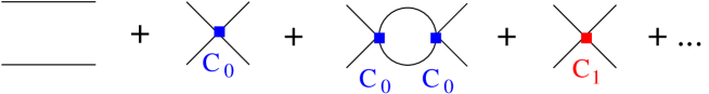
Figure 1: Diagrams contributing to the matrix element on the l.h.s of Eq. (37) in perturbation theory. The first diagram corresponds to the free propagation of the fields $\Phi_{1,2}$.

Note that in the non-relativistic EFT the above matrix element can be calculated in perturbation theory. The pertinent diagrams are shown in Fig. 1. Using the Euclidean-space propagator in the non-relativistic EFT

$$\langle 0|T\Phi_{i}(x)\Phi_{i}^{\dagger}(y)|0\rangle=\int\frac{dp_{0}}{2\pi}\,\frac{1}{L^{3}}\sum_{\bf p}\frac{e^{ip_{0}(x_{0}-y_{0})+i{\bf p}({\bf x}-{\bf y})}}{2w({\bf p})(w({\bf p})+ip_{0})}\,,\quad\quad w({\bf p})=\sqrt{m^{2}+{\bf p}^{2}}\,,$$ (38)

for this matrix element we get:

$$\langle 0|{\cal O}(x_{0};{\bf P},{\bf k}){\cal O}^{\dagger}(y_{0};{\bf P},{\bf k})|0\rangle=L^{3}\int\frac{dP_{0}}{2\pi}\,e^{iP_{0}(x_{0}-y_{0})}\,\hskip 165.02606pt$$

$$\times\biggl{\{}\frac{-iL^{3}}{4w_{1}({\bf k})w_{2}({\bf k})(P_{0}-i(w_{1}({\bf k})+w_{2}({\bf k})))}-\frac{T}{(4w_{1}({\bf k})w_{2}({\bf k}))^{2}(P_{0}-i(w_{1}({\bf k})+w_{2}({\bf k})))^{2}}\biggr{\}},$$ (39)

where

$$w_{1}({\bf k})=\sqrt{m^{2}+\biggl{(}\frac{\bf P}{2}+{\bf k}\biggr{)}^{2}}\,,\quad\quad w_{2}({\bf k})=\sqrt{m^{2}+\biggl{(}\frac{\bf P}{2}-{\bf k}\biggr{)}^{2}}\,,$$ (40)

and $T$ is the forward scattering amplitude of the particles 1 and 2 in the moving frame (see Fig. 1):

$$T = C_{0}+C_{0}^{2}\frac{1}{L^{3}}\sum_{\bf l}\frac{1}{4w_{1}({\bf l})w_{2}({\bf l})(w_{1}({\bf l})+w_{2}({\bf l})+iP_{0})}+\cdots\,.$$ (41)

$$= C_{0}+C_{0}^{2}\frac{p^{*}}{8\pi^{5/2}\sqrt{s}\gamma\eta}\,Z_{00}^{\bf d}(1;s)+\cdots\,,$$

$$s=-(P_{0}^{2}+{\bf P}^{2})\,,\quad\gamma=\biggl{(}1+\frac{{\bf P}^{2}}{P_{0}^{2}}\biggr{)}^{-1/2}\,,\quad p^{*}=\sqrt{\frac{s}{4}-m^{2}}\,,\quad\eta=\frac{p^{*}L}{2\pi}\,,$$

where we have used Eqs. (25,2), and where we have retained only the S-wave contribution in the scattering matrix in order to simplify the discussion of the scalar form factor. Using Eqs. (13,21), the tree-level and bubble diagrams in Fig. 1 can be summed up to all orders. The result on the energy shell is given by

$$T=\frac{8\pi\sqrt{s}}{p^{*}\cot\delta(s)+p^{*}\cot\phi^{\bf d}(s)}\,,\quad\quad\tan\phi^{\bf d}(s)=-\frac{\pi^{3/2}\eta\gamma}{Z_{00}^{\bf d}(1;s)}\,,$$ (42)

where $\delta(s)=\delta_{0}(s)$ denotes the S-wave phase shift.

The eigenvalues are determined from the Gottlieb-Rummukainen equation (see section 2):

$$\delta(s)=-\phi^{\bf d}(s)+\pi n\,,\quad\quad s=s_{n}\,,\quad{\bf P}~{}\mbox{fixed.}$$ (43)

The quantity $T$ defined by Eq. (42) has poles at real values of $s=s_{n}$, i.e., at $P_{0}=P_{0n}=iE_{n}$ where $E_{n}=E_{n}({\bf P})=\sqrt{s_{n}+{\bf P}^{2}}$. In the vicinity of this pole, the quantity $T$ behaves as:

$$T\to\frac{32\pi\sin^{2}\delta(s_{n})}{\delta^{\prime}(s)+(\phi^{\bf d}(s_{n}))^{\prime}}\,\frac{\sqrt{s_{n}}}{E_{n}}\,\frac{1}{E_{n}+iP_{0}}+\mbox{regular terms}\,,$$ (44)

where the derivative is taken with respect to the variable $p^{*}$. Substituting now this expression into Eq. (3), performing the integral over $P_{0}$ and taking into account the fact that the “free” poles at $P_{0}=i(w_{1}({\bf k})+w_{2}({\bf k}))$ cancel in the integrand, the final expression for the matrix element in Eq. (3) for $x_{0}-y_{0}>0$ reads:

$$\langle 0|{\cal O}(x_{0};{\bf P},{\bf k}){\cal O}^{\dagger}(y_{0};{\bf P},{\bf k})|0\rangle = L^{3}\sum_{n}\frac{32\pi\sin^{2}\delta(s_{n})}{\delta^{\prime}(s)+(\phi^{\bf d}(s_{n}))^{\prime}}\,\frac{\sqrt{s_{n}}}{E_{n}}\,$$ (45)

$$\times \frac{e^{-E_{n}(x_{0}-y_{0})}}{(4w_{1}({\bf k})w_{2}({\bf k}))^{2}(E_{n}-w_{1}({\bf k})-w_{2}({\bf k}))^{2}}\,.$$

Comparing this expression with Eq. (37), one reads off:

$$|\langle 0|{\cal O}(0;{\bf P},{\bf k})|E_{n}({\bf P})\rangle| = L^{3/2}\biggl{(}\frac{32\pi\sin^{2}\delta(s_{n})}{|\delta^{\prime}(s)+(\phi^{\bf d}(s_{n}))^{\prime}|}\,\frac{\sqrt{s_{n}}}{E_{n}}\biggr{)}^{1/2}\,$$ (46)

$$\times \frac{1}{4w_{1}({\bf k})w_{2}({\bf k})}\,\frac{1}{|E_{n}-w_{1}({\bf k})-w_{2}({\bf k})|}\,.$$

Next, we turn to the determination of the form factor in the time-like region. To this end, we have to consider the amplitude of pair creation from the vacuum in the presence of an external field $A(x)$, at the first order in the coupling $e$. This matrix element is described by

$$\langle 0|{\cal O}(x_{0},{\bf P},{\bf k})\,{\cal L}_{\sf A}(0)|0\rangle=eA(0)F[{\bf k},{\bf P};x_{0}]\,,\quad\quad x_{0}>0\,.$$ (47)

We evaluate the quantity $F$ in perturbation theory. The pertinent diagrams are shown in Fig. 2. Summing up all bubbles yields:

$$F[{\bf k},{\bf P};x_{0}]=\bar{F}(t)\int\frac{dP_{0}}{2\pi i}\frac{e^{iP_{0}x_{0}}}{4w_{1}({\bf k})w_{2}({\bf k})(P_{0}-i(w_{1}({\bf k})+w_{2}({\bf k})))}\,\frac{p^{*}\cot\delta(s)}{p^{*}\cot\delta(s)+p^{*}\cot\phi^{\bf d}(s)}\,,$$ (48)

where the quantity $\bar{F}(t)$ can be read off the Lagrangian in Eq. (34) at tree level

$$\bar{F}(t) = 1+D_{1}t+O(t^{2})\,,\quad\quad t=(k_{1}+k_{2})^{2}\,,$$

$$k_{1}^{\mu} = \biggl{(}w_{1}({\bf k}),\frac{\bf P}{2}+{\bf k}\biggr{)}\,,\quad k_{2}^{\mu}=\biggl{(}w_{2}({\bf k}),\frac{\bf P}{2}-{\bf k}\biggr{)}\,.$$ (49)

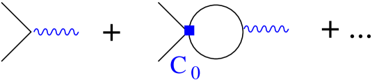
Figure 2: Diagrams contributing to the vertex function. The wiggly line corresponds to the external field $A(x)$.

Using Eq. (44), we may now perform the integration over the variable $P_{0}$ in Eq. (48), with the result

$$F[{\bf k},{\bf P};x_{0}]=\bar{F}(t)\sum_{n}\frac{e^{-E_{n}x_{0}}}{4w_{1}({\bf k})w_{2}({\bf k})(w_{1}({\bf k})+w_{2}({\bf k})-E_{n})}\,\frac{4p^{*}\cot\delta(s_{n})\sin^{2}\delta(s_{n})}{(\delta^{\prime}(s)+(\phi^{\bf d}(s_{n}))^{\prime})E_{n}}\,.$$ (50)

On the other hand, the matrix element in Eq. (47) has the following representation:

$$\langle 0|{\cal O}(x_{0},{\bf P},{\bf k})\,{\cal L}_{\sf A}(0)|0\rangle=eA(0)\sum_{n}e^{-E_{n}x_{0}}\langle 0|{\cal O}(0,{\bf P},{\bf k})|E_{n}({\bf P})\rangle\langle E_{n}({\bf P})|j(0)|0\rangle\,.$$ (51)

Using Eqs. (46), (50) and (51), we get

$$|\langle E_{n}({\bf P})|j(0)|0\rangle|=L^{-3/2}|\bar{F}(t)|\frac{p^{*}|\cos\delta(s_{n})|}{(2\pi\sqrt{s}E_{n})^{1/2}}\,\frac{1}{|\delta^{\prime}(s)+(\phi^{\bf d}(s_{n}))^{\prime}|^{1/2}}\,.$$ (52)

This is the expression of the matrix element in a finite volume. It should be compared with its counterpart in the infinite volume, which is obtained by using Watson’s theorem:

$$\langle k_{1},k_{2};\mbox{\sf out}|j(0)|0\rangle=F(t)\,,\quad\quad|F(t)|=|\bar{F}(t)\cos\delta(s)|\,.$$ (53)

From Eqs. (52) and (53) we finally get:

$$|F(t)|^{2}=|L^{3/2}\langle E_{n}({\bf P})|j(0)|0\rangle|^{2}\frac{2\pi\sqrt{s}E_{n}}{(p^{*})^{2}}\,|\delta^{\prime}(s)+(\phi^{\bf d}(s_{n}))^{\prime}|\,.$$ (54)

This expression allows one to extract the absolute value of a scalar form factor in the time-like region from the measured matrix element $\langle E_{n}({\bf P})|j(0)|0\rangle$ in a finite volume. Since the phase of this form factor, which is determined by Watson’s theorem, is also measurable on the lattice, we finally conclude that the real and imaginary parts of the form factor can be measured on the lattice in the elastic region.

In the rest frame, the expression in Eq. (54) is similar to the expression obtained in Ref. [21], apart from a difference in a kinematical factor which is related to the fact that there a vector form factor instead of a scalar one was considered. It can be also shown that, by using our method, one exactly reproduces the Lüscher-Lellouch formula in moving frames [37, 20, 38].

4 Extraction of resonance matrix elements in a finite volume

Having considered the case of the form factor in the time-like region in great detail, we turn to the extraction of the resonance form factor. The part of the Lagrangian that describes the interaction with the external scalar field $A(x)$, looks now as follows:

$$\bar{\cal L}_{\sf A}=A(x)\bar{j}(x)=e_{1}A(\Phi_{1}^{\dagger}\Phi_{1}+\cdots)+e_{2}A(\Phi_{2}^{\dagger}\Phi_{2}+\cdots)+E_{0}A(\Phi_{1}^{\dagger}\Phi_{2}^{\dagger}\Phi_{1}\Phi_{2}+\cdots)\,,$$ (55)

where $e_{1,2},E_{0},\cdots$ denote low-energy couplings, and the ellipses stand for the terms with higher derivatives. It is seen that, in general, the current $\bar{j}(x)$ consists of one-body currents and a two-body current, whose coupling at lowest order is given by $E_{0}$.

We make the following choice for the resonance field operators:

$${\cal O}(x_{0};{\bf P}) = \int_{-L/2}^{L/2}d^{3}{\bf x}\,e^{-i{\bf P}{\bf x}}\,\Phi_{1}(x_{0},{\bf x})\Phi_{2}(x_{0},{\bf x})\,,$$

$${\cal O}^{\dagger}(y_{0};{\bf Q}) = \int_{-L/2}^{L/2}d^{3}{\bf y}\,e^{i{\bf Q}{\bf y}}\,\Phi_{1}^{\dagger}(y_{0},{\bf y})\Phi_{2}^{\dagger}(y_{0},{\bf y})\,.$$ (56)

The first-order scattering amplitude of the particles 1 and 2 in the external field $A(x)$ can again be calculated using perturbation theory. The pertinent diagrams are depicted in Fig. 3. The result of the calculation is (cf. with Eqs. (47,48)):

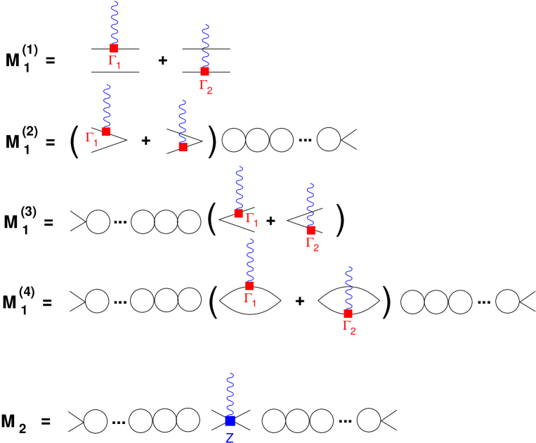
Figure 3: The diagrams describing the quantity $M=M_{1}+M_{2}$ in Eq. (58). $M_{1}$ and $M_{2}$ correspond to the contributions of the one- and two-body currents, respectively. The wiggly line corresponds to the external field $A(x)$. All initial- and final-state interactions are summed up in the bubble chains.

$$\langle 0|{\cal O}(x_{0},{\bf P})\bar{\cal L}_{\sf A}(0){\cal O}^{\dagger}(y_{0},{\bf Q})|0\rangle=A(0)\bar{F}({\bf P},{\bf Q},x_{0},y_{0})\,,\quad\quad x_{0}>0,~{}y_{0}<0\,,$$ (57)

where

$$F({\bf P},{\bf Q},x_{0},y_{0})=\frac{1}{L^{6}}\sum_{{\bf p},{\bf q}}\int\frac{dP_{0}}{2\pi i}\,\frac{dQ_{0}}{2\pi i}\,\frac{e^{iP_{0}x_{0}}\,M(P_{0},{\bf P},{\bf p};Q_{0},{\bf Q},{\bf q})\,e^{-iQ_{0}y_{0}}}{4w_{1}w_{2}(P_{0}-i(w_{1}+w_{2}))4w_{1}^{\prime}w_{2}^{\prime}(Q_{0}-i(w_{1}^{\prime}+w_{2}^{\prime}))}\,,$$ (58)

where

$$w_{1}=\sqrt{m^{2}+\biggl{(}\frac{\bf P}{2}+{\bf p}\biggr{)}}\,,\quad w_{2}=\sqrt{m^{2}+\biggl{(}\frac{\bf P}{2}-{\bf p}\biggr{)}}\,,\quad$$

$$w_{1}^{\prime}=\sqrt{m^{2}+\biggl{(}\frac{\bf Q}{2}+{\bf q}\biggr{)}}\,,\quad w_{2}^{\prime}=\sqrt{m^{2}+\biggl{(}\frac{\bf Q}{2}-{\bf q}\biggr{)}}\,.$$ (59)

The diagrammatic expansion of the quantity $M$ is shown in Fig. 3. It consists of the contributions corresponding to the one-body and two-body currents (see Eq. (55)). Retaining only the S-wave contribution in the initial- and final-state rescattering amplitudes, we get:

$$M=M_{1}+M_{2}\,,\quad\quad M_{1}=M_{1}^{(1)}+M_{1}^{(2)}+M_{1}^{(3)}+M_{1}^{(4)}\,,$$ (60)

where

$$M_{1}^{(1)} = (2w_{2})\Gamma_{1}\biggl{(}\frac{\bf P}{2}+{\bf p},\frac{\bf Q}{2}+{\bf q}\biggr{)}L^{3}\delta_{\frac{\bf P}{2}-{\bf p},\frac{\bf Q}{2}-{\bf q}}+(2w_{1})\Gamma_{2}\biggl{(}\frac{\bf P}{2}-{\bf p},\frac{\bf Q}{2}-{\bf q}\biggr{)}L^{3}\delta_{\frac{\bf P}{2}+{\bf p},\frac{\bf Q}{2}+{\bf q}}\,,$$

$$M_{1}^{(2)} = \frac{\Gamma_{1}\biggl{(}\dfrac{\bf P}{2}+{\bf p},{\bf Q}-\dfrac{\bf P}{2}+{\bf p}\biggr{)}}{2\tilde{w}_{1}(\tilde{w}_{1}+w_{2}+iQ_{0})}\,S(q^{*})+\frac{\Gamma_{2}\biggl{(}\dfrac{\bf P}{2}-{\bf p},{\bf Q}-\dfrac{\bf P}{2}-{\bf p}\biggr{)}}{2\tilde{w}_{2}(\tilde{w}_{2}+w_{1}+iQ_{0})}\,S(q^{*})+\bar{M}_{1}^{(2)}\,,$$

$$M_{1}^{(3)} = \frac{\Gamma_{1}\biggl{(}{\bf P}-\dfrac{\bf Q}{2}+{\bf q},\dfrac{\bf Q}{2}+{\bf q}\biggr{)}}{2\tilde{w}_{1}^{\prime}(\tilde{w}_{1}^{\prime}+w_{2}^{\prime}+iP_{0})}\,S(p^{*})+\frac{\Gamma_{2}\biggl{(}{\bf P}-\dfrac{\bf Q}{2}-{\bf q},\dfrac{\bf Q}{2}-{\bf q}\biggr{)}}{2\tilde{w}_{2}^{\prime}(\tilde{w}_{2}^{\prime}+w_{1}^{\prime}+iP_{0})}\,S(p^{*})+\bar{M}_{1}^{(3)}\,,$$

$$M_{1}^{(4)} = \frac{1}{L^{3}}\sum_{\bf l}\frac{S(p^{*})(\Gamma_{1}({\bf P}-{\bf l},{\bf Q}-{\bf l})+\Gamma_{2}({\bf P}-{\bf l},{\bf Q}-{\bf l}))S(q^{*})}{8w({\bf P}-{\bf l})w({\bf Q}-{\bf l})w({\bf l})(w({\bf Q}-{\bf l})+w({\bf l})+iQ_{0})(w({\bf P}-{\bf l})+w({\bf l})+iP_{0})}$$ (61)

$$+ \bar{M}_{1}^{(4)}\,.$$

In the above expressions, $\bar{M}_{1}^{(2)}$ and $\bar{M}_{1}^{(3)}$ do not contain denominators linear in $Q_{0}$ and $P_{0}$, respectively, but still include the factors $S(q^{*}),S(p^{*})$. The quantity $\bar{M}_{1}^{(4)}$ contains at most one energy denominator and both $S(q^{*})$ and $S(p^{*})$. These quantities emerge, because initial- and final-state rescattering occurs, in general, off the energy shell. Further,

$$\tilde{w}_{1} = \sqrt{m^{2}+\biggl{(}{\bf Q}-\frac{\bf P}{2}+{\bf p}\biggr{)}^{2}}\,,\quad\tilde{w}_{2}=\sqrt{m^{2}+\biggl{(}{\bf Q}-\frac{\bf P}{2}-{\bf p}\biggr{)}^{2}}\,,\quad$$

$$\tilde{w}_{1}^{\prime} = \sqrt{m^{2}+\biggl{(}{\bf P}-\frac{\bf Q}{2}+{\bf q}\biggr{)}^{2}}\,,\quad\tilde{w}_{2}^{\prime}=\sqrt{m^{2}+\biggl{(}{\bf P}-\frac{\bf Q}{2}-{\bf q}\biggr{)}^{2}}\,,$$ (62)

$$S(p^{*}) = \frac{8\pi\sqrt{s}}{p^{*}\cot\delta(s)+p^{*}\cot\phi^{\bf d}(s)}\,,\quad S(q^{*})=\frac{8\pi\sqrt{s}}{q^{*}\cot\delta(s^{\prime})+q^{*}\cot\phi^{{\bf d}^{\prime}}(s^{\prime})}\,,$$

$$s = -(P_{0}^{2}+{\bf P}^{2})\,,\quad s^{\prime}=-(Q_{0}^{2}+{\bf Q}^{2})\,,$$

$$p^{*} = \sqrt{\frac{s}{4}-m^{2}}\,,\quad q^{*}=\sqrt{\frac{s^{\prime}}{4}-m^{2}}\,,\quad{\bf d}=\frac{2\pi{\bf P}}{L}\,,\quad{\bf d}^{\prime}=\frac{2\pi{\bf Q}}{L}\,,$$ (63)

and the $\Gamma_{1,2}$ denote the tree-level interaction vertices of the external field $A(x)$ with the fields $\Phi_{1,2}$.

After projection onto S-waves, the two-body current leads to the following contribution (see Fig. 3):

$$M_{2} = \frac{p^{*}\cot\delta(s)}{p^{*}\cot\delta(s)+p^{*}\cot\phi^{\bf d}(s)}\,Z(iP_{0},{\bf P};iQ_{0},{\bf Q})\,\frac{q^{*}\cot(s^{\prime})}{q^{*}\cot\delta(s^{\prime})+q^{*}\cot\phi^{{\bf d}^{\prime}}(s^{\prime})}$$ (64)

$$+ \mbox{regular functions in $P_{0}$ or $Q_{0}$},,$$

where the quantity $Z$ is a low-energy polynomial.

It can be straightforwardly checked that the sum of all terms in the integrand in Eq. (58) do not have singularities at the free two-particle levels. The only singularities are simple poles that correspond to the energy levels in the full theory and emerge after the summation of the bubble chains. Taking this fact into account and performing the contour integration in the variables $P_{0},Q_{0}$ by using Cauchy’s theorem, we get:

$$F({\bf P},{\bf Q},x_{0},y_{0}) = \frac{1}{L^{6}}\sum_{{\bf p},{\bf q}}\sum_{n,m}\frac{32\pi\sin^{2}\delta(s_{n})\sqrt{s_{n}}e^{-E_{n}x_{0}}}{4w_{1}w_{2}E_{n}(w_{1}+w_{2}-E_{n})(\delta^{\prime}(s_{n})+(\phi^{\bf d}(s_{n}))^{\prime})}\,V_{nm}({\bf P};{\bf Q})$$ (65)

$$\times \frac{32\pi\sin^{2}\delta(s_{m})\sqrt{s_{m}}e^{E_{m}y_{0}}}{4w_{1}^{\prime}w_{2}^{\prime}E_{m}(w_{1}^{\prime}+w_{2}^{\prime}-E_{m})(\delta^{\prime}(s_{m})+(\phi^{\bf d}(s_{m}))^{\prime})}\,,$$

where

$$V_{nm}({\bf P};{\bf Q}) \!=\! \frac{1}{L^{3}}\sum_{\bf l}\frac{\Gamma_{1}({\bf P}-{\bf l},{\bf Q}-{\bf l})+\Gamma_{2}({\bf P}-{\bf l},{\bf Q}-{\bf l})}{8w({\bf P}-{\bf l})w({\bf Q}-{\bf l})w({\bf l})(w({\bf P}-{\bf l})+w({\bf l})-E_{n})(w({\bf Q}-{\bf l})+w({\bf l})-E_{m})}$$ (66)

$$\!+\! \frac{p^{*}_{n}\cot\delta(s_{n})}{8\pi\sqrt{s_{n}}}\,Z(E_{n},{\bf P};E_{m},{\bf Q})\frac{q^{*}_{m}\cot\delta(s_{m})}{8\pi\sqrt{s_{m}}}$$

with $p^{*}_{n}=p^{*}(s=s_{n})$, $q^{*}_{m}=q^{*}(s^{\prime}=s_{m})$. In Eq. (65), the Gottlieb-Rummukainen equation will be further used to remove the summations over ${\bf p},{\bf q}$:

$$\frac{1}{L^{3}}\sum_{\bf p}\frac{1}{4w_{1}w_{2}(w_{1}+w_{2}-E_{n})}=\frac{p_{n}^{*}\cot\delta(s_{n})}{8\pi\sqrt{s_{n}}}\,.$$ (67)

On the other hand, inserting a full set of the eigenstates of the full Hamiltonian, we get

$$F({\bf P},{\bf Q},x_{0},y_{0}) = \sum_{n,m}\langle 0|{\cal O}(0;{\bf P})|E_{n}({\bf P})\rangle e^{-E_{n}x_{0}}\langle E_{n}({\bf P})|\bar{j}(0)|E_{m}({\bf Q})\rangle$$ (68)

$$\times e^{E_{m}y_{0}}\langle E_{m}({\bf Q})|{\cal O}^{\dagger}(0;{\bf Q})|0\rangle\,.$$

Further, by using perturbation theory, it is straightforward to show that

$$|\langle 0|{\cal O}(0;{\bf P})|E_{n}({\bf P})\rangle|^{2}=L^{3}\,\frac{\cos^{2}\delta(s_{n})}{\delta^{\prime}(s_{n})+(\phi^{\bf d}(s_{n}))^{\prime}}\,\frac{(p_{n}^{*})^{2}}{2\pi E_{n}({\bf P})\sqrt{s_{n}}}\,.$$ (69)

Taking $n=m$, we readily obtain:

$$\langle E_{n}({\bf P})|\bar{j}(0)|E_{n}({\bf Q})\rangle=\frac{(4\sin\delta(s_{n}))^{2}}{\delta^{\prime}(s_{n})+(\phi^{\bf d}(s_{n}))^{\prime}}\,\frac{2\pi\sqrt{s_{n}}}{L^{3}\sqrt{E_{n}({\bf P})E_{n}({\bf Q})}}\,V_{nn}({\bf P};{\bf Q})\,.$$ (70)

Independently, one may extract the resonance matrix element in the infinite-volume non-relativistic EFT by using the procedure described in the introduction. The result is given by:

$$\langle{\bf P}|\bar{j}(0)|{\bf Q}\rangle=B_{R}\,V^{\infty}({\bf P};{\bf Q})\,,\quad\quad s,s^{\prime}\to s_{R}=4(m^{2}+p_{R}^{2})\,,$$ (71)

where

$$\frac{8\pi\sqrt{s}}{p\cot\delta(p)-ip}\to\frac{B_{R}}{s_{R}-s}\,,\quad\quad B_{R}=-\frac{64\pi\sqrt{s_{R}}p_{R}}{2p_{R}h^{\prime}(p_{R}^{2})-i}\,,$$ (72)

and

$$h(p^{2})=p\cot\delta(p)=-\frac{1}{a}+\frac{1}{2}\,rp^{2}+\cdots\,,$$ (73)

and $V^{\infty}$ is obtained from $V_{nm}$ through $E_{n}\to P_{0}$, $E_{m}\to Q_{0}$, $s,s^{\prime}\to s_{R}$ and further replacing the discrete sum by integration over the variable ${\bf l}$.

At this stage, we can visualize the problem inherent to the extraction of the resonance matrix elements. On the lattice, one may measure the quantity $\langle E_{n}({\bf P})|\bar{j}(0)|E_{n}({\bf Q})\rangle$ and extract the quantity $V_{nn}$ through Eq. (70). If we were dealing with a stable bound state, in the infinite volume $V_{nn}\to V^{\infty}$, up to exponentially small corrections. Multiplying with the pertinent bound-state renormalization factor, we would directly arrive at the matrix element of the current $\bar{j}(0)$, sandwiched between the stable bound-state vectors. However, we are dealing with a resonance and not with a stable bound state. This means that:

• No single $E_{n}$ corresponds to a resonance. We have to formulate a procedure for the analytic continuation of the matrix elements into the complex plane.

• The quantity $V_{nn}$ does not have a well-defined limit as $L\to\infty$ and $E_{n}$ above the two-particle threshold. The 1-loop diagram with an external field, which contributes to the $M_{1}^{(4)}$, is the culprit. On the contrary, the contribution from the two-body current, $Z$, is a low-energy polynomial and does not cause any problem.

In the following sections, we shall explicitly address both of these problems.

5 Analytic continuation and fixed points

In order to avoid kinematical complications, let us first consider the form factor at a zero momentum transfer ${\bf P}={\bf Q}=0$. The quantity $V_{nn}$ is then a function of a single variable $p=\sqrt{E_{n}^{2}/4-m^{2}}$. The questions can be now formulated as follows:

• How does one perform the analytic continuation $p\to p_{R}$ in the quantity $V_{nn}(p)$?

• How does one perform the infinite volume limit $L\to\infty$?

We shall see below that these two questions are intimately related.

Let us imagine for a moment that the contribution from the loop diagrams vanishes, so that the quantity $V_{nn}$ is given by the two-body current diagram $Z$ only. Then, the answers to the above equations are trivial. The quantity $Z$ is a polynomial in the variable $p^{2}$: $Z=Z_{0}+Z_{1}p^{2}+\cdots$. So, one has to first fit the coefficients $Z_{0},Z_{1},\cdots$ to the lattice data, and then simply substitute $p^{2}\to p_{R}^{2}$. The result gives the analytic continuation $Z(p^{2})\to Z(p_{R}^{2})$. Moreover, since $Z(p^{2})$ is $L$-independent, so is $Z(p_{R}^{2})$, and the final result does not depend on the energy level $n$ we started from.

Let us now see what changes when the one-body current contribution is also included. To this end, we first study the analytic continuation of the Lüscher equation into the complex plane. To ease notation, we restrict ourselves to S-waves and write down the equation (in the CM frame) in the following form:

$$\frac{h(p^{2})}{p}=\cot\delta(p)=\frac{1}{\pi^{3/2}\eta}\,Z_{00}(1,\eta^{2})\,.$$ (74)

On the real axis,

$$\eta=\frac{pL}{2\pi}\,,$$ (75)

and Eq. (74) determines the energy levels given the scattering phase (or vice versa). Let us now look for solutions of this equation for complex values of $p$. The quantity $h(p^{2})$ is a low-energy polynomial in $p^{2}$, so the analytic continuation is trivial. Furthermore, the function $Z_{00}(1,\eta^{2})$ is a meromorphic function of the variable $\eta^{2}$. Thus, for any given complex value of $p$, the solutions of Eq. (74) determine the trajectories $\eta_{n}(p),~{}n=0,1,\ldots$ , in the complex plane (we remind the reader that the solutions are not unique). As $p\to p_{R}$ in the $p$-plane, $\eta_{n}(p)\to\eta_{nR}$ in the $\eta$-plane and Eq. (75) becomes a relation that defines $L$. Our first task is to find all $\eta_{nR}$.

It is instructive to begin from the 1+1-dimensional case [23]. The counterpart of Eq. (74) in this case reads:

$$\cot\delta(p)=-\cot\pi\eta\,.$$ (76)

The solution of this equation with respect to $\eta$ reads:

$$\eta=-\frac{i}{2\pi}\,\ln\frac{-1+ix}{1+ix}\,,\quad\quad x=\cot\delta(p)\,.$$ (77)

On the resonance position, we have $p\to p_{R}$ and $\cot\delta(p)\to-i$. Writing $x=-i+\epsilon$, we get

$$\eta\sim\frac{1}{2\pi}\arg i\epsilon-\frac{i}{2\pi}\,\ln\frac{|\epsilon|}{2}+O(\epsilon)\,,\quad\mbox{as}~{}p\to p_{R}\,.$$ (78)

If we exclude those paths connecting $p$ and $p_{R}$ in the $p$-plane, which wind around $p_{R}$ infinitely many times, then

$$\lim_{p\to p_{R}}\mbox{Re}\,\eta(p)<\infty\,,\quad\quad\mbox{Im}\,\eta(p)\to-\infty,\quad\mbox{as}~{}p\to p_{R}\,.$$ (79)

Recalling the definition of the variable $\eta$ (see Eq. (75)), one may interpret the above result (in a loose sense) as the equivalence of the mass-shell limit for a resonance ($p\to p_{R}$) and the infinite-volume limit. The same is true for a stable bound state: its energy is volume-independent up to exponentially small corrections, so the walls can be safely moved to infinity. Our result shows that the same statement holds for a resonance pole (in the 1+1 dimensional case). On the contrary, the discrete spectrum above the two-particle threshold is determined by the presence of the walls. If one moves the walls to infinity ($L\to\infty$), each given energy level collapses toward threshold. The spectrum becomes continuous in this limit.

What does change in the 3+1 dimensional case? There are so-called finite fixed points with $|\eta_{nR}|<\infty$, in addition to the fixed points at infinity which are given by Eq. (79). In order to see this, we provide below a numerical solution of Eq. (74) (an analytical solution is not available in the $3+1$-dimensional case).

The fixed points are the solutions of the equation

$$Z_{00}(1;\eta^{2})+i\pi^{3/2}\eta=0\,.$$ (80)

If $\mbox{Im}\,\eta<0$, one may use the following representation of the zeta-function:

$$Z_{00}(1;\eta^{2})=\pi^{3/2}\eta\,\biggl{\{}-i+\sum_{|{\bf n}|\neq 0}\frac{1}{2\pi\eta|{\bf n}|}\,e^{-2\pi i\eta|{\bf n}|}\biggr{\}}\,,\quad\quad{\bf n}\in\mathbb{Z}^{3}\,.$$ (81)

By using Eq. (81), Eq. (80) can be rewritten as

$$6e^{-2\pi i\eta}+\frac{12}{\sqrt{2}}\,e^{-2\pi i\sqrt{2}\eta}+\Sigma(\eta)=0\,,\quad\quad\Sigma(\eta)=\sum_{|{\bf n}|\geq\sqrt{3}}\frac{1}{|{\bf n}|}\,e^{-2\pi i\eta|{\bf n}|}\,.$$ (82)

This equation has infinitely many solutions. In order to verify this statement, first assume that $\Sigma(\eta)=0$. In this approximation, there exists a tower of finite fixed poles parameterized as

$$\eta_{nR}^{(0)}=\frac{n+\frac{1}{2}}{\sqrt{2}-1}-\frac{i\ln 2}{4\pi(\sqrt{2}-1)}\,,\quad\quad n=-\infty,\cdots,-1,0,1,\cdots,\infty\,.$$ (83)

Finally, the equation (82) can be rewritten as

$$\eta=\frac{n+\frac{1}{2}}{\sqrt{2}-1}-\frac{i\ln 2}{4\pi(\sqrt{2}-1)}-\frac{i}{2\pi(\sqrt{2}-1)}\,\ln\biggl{(}1+\frac{\sqrt{2}}{12}\,e^{2\pi i\sqrt{2}\eta}\,\Sigma(\eta)\biggr{)}\,.$$ (84)

This equation can be easily solved by iteration, starting from $\eta=\eta_{nR}^{(0)}$. Note that the series for $\Sigma(\eta)$ contains exponentially suppressed terms and converges very fast. So, truncating the sum at some $|{\bf n}|=n_{\sf max}$ can be justified. The numerical solutions indeed exist and are shown in Fig. 4.

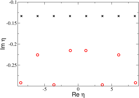
Figure 4: Positions of the finite fixed points in the complex $\eta$-plane. The crosses and circles denote $\eta_{nR}^{(0)}$ and $\eta_{nR}$, respectively. The plot is symmetric with respect to the imaginary axis.

Enter the culprit. What are the implications of the above result for the calculation of resonance matrix elements? Consider a simplified expression for $V_{nn}({\bf 0},{\bf 0})$ in Eq. (66), setting $\Gamma_{1}=1$, $\Gamma_{2}=0$ and $Z=0$ (the low-energy polynomials in the numerator do not alter the analytic properties of the diagram we are interested in, and the part containing $Z$ is trivial and was considered already). All we have to consider is the expression

$$V_{nn}({\bf 0},{\bf 0}) = \frac{1}{L^{3}}\sum_{\bf l}\frac{1}{(2w({\bf l}))^{3}(2w({\bf l})-E_{n})^{2}}=\frac{d}{dE}\biggl{(}\frac{p}{8\pi E^{2}}\,\frac{Z_{00}(1;\eta^{2})}{\pi^{3/2}\eta}\biggr{)}\biggr{|}_{E=E_{n}}+\cdots$$ (85)

$$= -\biggl{(}\frac{m^{2}-p^{2}}{8\pi E^{3}p^{2}}\,p\cot\phi(\eta)-\frac{1}{32\pi Ep}\,(1+\cot^{2}\phi(\eta))\,\eta\phi^{\prime}(\eta)\biggr{)}\biggr{|}_{E=E_{n}}+\cdots\,,$$

$$= \biggl{(}\frac{m^{2}-p^{2}}{8\pi E^{3}p^{2}}\,p\cot\delta(p)+\frac{1}{32\pi Ep}\,(1+\cot^{2}\delta(p))\,\eta\phi^{\prime}(\eta)\biggr{)}\biggr{|}_{E=E_{n}}+\cdots\,,$$

where $\phi(\eta)=\phi^{{\bf d}={\bf 0}}(E^{2})$, $E=2\sqrt{m^{2}+p^{2}}$, and the ellipses stand for the terms which vanish exponentially with $L$. In the last line of Eq. (85), Lüscher’s equation $\cot\phi(\eta)=-\cot\delta(p)$ was used. The quantity $V_{nn}({\bf 0},{\bf 0})$ is a function of the variable $p$, so one can write $V_{nn}({\bf 0},{\bf 0})=V_{nn}(p)$. It is now legitimate to ask how the analytic continuation of the above expression in $p$ is performed and what is the result of this continuation. The expression in Eq. (85) consists of two terms. It can be verified directly that the first term is a low-energy polynomial in $p^{2}$ (up to a trivial overall factor $p^{-2}$). The analytic continuation of this term is straightforward and leads to

$$\frac{m^{2}-p^{2}}{8\pi E^{3}p^{2}}\,p\cot\delta(p)\to-i\frac{m^{2}-p_{R}^{2}}{8\pi s_{R}^{3/2}p_{R}}\,,\quad\quad\mbox{as}~{}p\to p_{R}\,.$$ (86)

It is easy to check that this result exactly coincides with the result for the loop diagram calculated in the infinite volume (i.e., replacing summation by integration in Eq. (85)), on the second sheet. Consequently, if the second term, continued to $p=p_{R}$, vanishes, the analytic continuation of the whole vertex diagram to the pole on the second sheet will yield the same vertex evaluated in the infinite volume. This would be the statement that we are after.

Let us assume for a moment that it is possible to find a procedure to perform such an analytic continuation in the second term of Eq. (85). We choose some path in the complex $p$-plane approaching the pole at $p=p_{R}$. Suppose first that, moving along this path, the variable $\eta=\eta(p)$ approaches the infinite fixed point $|\mbox{Re}\,\eta_{nR}|<\infty$, $\mbox{Im}\,\eta_{nR}\to-\infty$. Using the representation for the zeta-function given in Eq. (81), it can be easily checked that the second term in Eq. (85) indeed vanishes if $\eta$ tends to the infinite fixed point.

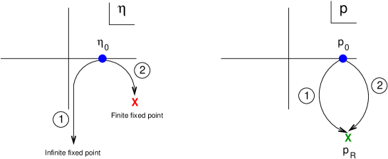
Figure 5: Two different paths in the $\eta$-plane and corresponding paths in the $p$-plane. It is seen that the paths converge to the same point $p_{R}$ in the $p$-plane.

Imagine now a path that ends at a finite fixed point. Parameterizing this path as

$$\cot\phi(\eta)+i=\lambda(\eta-\eta_{nR})+O((\eta-\eta_{nR})^{2})\,,$$ (87)

where $\lambda$ is a finite complex constant. Then, in the vicinity of the fixed point,

$$\phi(\eta)\propto\ln(\eta-\eta_{nR})+\mbox{const}+O(\eta-\eta_{nR})\,,\quad\quad\phi^{\prime}(\eta)\propto\frac{1}{\eta-\eta_{nR}}+\mbox{const}+O(\eta-\eta_{nR})\,.$$ (88)

From the above equations it is evident that the product $\eta(1+\cot^{2}\phi(\eta))\phi^{\prime}(\eta)$, rather than vanishing, tends to a constant at the finite fixed point. In other words, if during the analytic continuation, the variable $\eta$ gets caught by a finite fixed point, the result of the analytic continuation is different from the vertex function in the infinite volume and one is in trouble.

In order to understand this result better, let us consider some point $\eta_{0}$ on the real axis and two paths, connecting $\eta_{0}$ to an infinite and to a finite fixed points, respectively (see Fig. 5). These paths are mirrored by pertinent paths in the $p$-plane. Since we have assumed that there is only one resonance pole at $p=p_{R}$, both paths in the $p$-plane start at the same point $p=p_{0}$ corresponding to $\eta=\eta_{0}$ and end at the same point $p=p_{R}$. The result of the analytic continuation is, however, different along these paths, rendering an unambiguous determination of the vertex function at $p=p_{R}$ impossible.

The problem, which was discussed above, looks complicated but has a particularly simple solution. Let us go back to the last line of Eq. (85). It is immediately seen that the ambiguity is caused by the expression $\eta\phi^{\prime}(\eta)$, which is contained in the second term and depends on the energy level index $n$. Moreover, the form of this expression is universal (it does not depend on the interaction). Consequently, measuring the vertex function for two different energy levels $n$ and $m$, and forming the linear combination,

$$\bar{V}(p)=\frac{V_{nn}(p)\eta_{m}\phi^{\prime}(\eta_{m})-V_{mm}(p)\eta_{n}\phi^{\prime}(\eta_{n})}{\eta_{m}\phi^{\prime}(\eta_{m})-\eta_{n}\phi^{\prime}(\eta_{n})}\,,$$ (89)

one may immediately ensure that the culprit disappears. Namely, $\bar{V}(p)$ is a low-energy polynomial in the variable $p^{2}$ up to a factor $p^{-2}$, it does not depend on the energy level (up to exponentially suppressed contributions), and its analytic continuation $p\to p_{R}$ into the complex $p$-plane yields the infinite-volume vertex function. To conclude, the problem with the analytic continuation was circumvented by measuring the matrix elements for two different energy levels.

Finally, we would like to note that the problem is milder in the case of 1+1 dimensions, see Ref. [23]. First, there are no finite fixed points and no ambiguity emerges. Second, in Ref. [23] it has been shown that the problematic contributions in 1+1 dimensions can be fit by a polynomial in $p$ (not $p^{2}$) with $n$-dependent coefficients, so the analytic continuation still can be performed (although it is a more subtle affair now, see Ref. [23] for the details). No similar statement exists in the case of 3+1 dimensions. The subtraction trick can be used in 1+1 dimensions as well, making the fit more straightforward (at the cost of measuring two energy levels instead of one).

6 Matrix elements at nonzero momentum transfer

We finally turn to the resonance matrix elements for non-zero momentum transfer. It is convenient to work in the Breit frame ${\bf P}=-{\bf Q}$. The vertex function in the infinite volume using dimensional regularization is given by (we again neglect the numerators which do not affect the analytic properties):

$$I = \int\frac{d^{d}{\bf l}}{(2\pi)^{d}}\,\frac{1}{8w({\bf l})w({\bf P}-{\bf l})w({\bf P}+{\bf l})}\,\frac{1}{(w({\bf P}-{\bf l})+w({\bf l})-P_{0})(w({\bf P}+{\bf l})+w({\bf l})-P_{0})}\,,$$

$$p^{*} = \sqrt{\frac{s}{4}-m^{2}}\,,\quad\quad s=P_{0}^{2}-{\bf P}^{2}\,,$$ (90)

where the $P_{0}\to P_{0}+i0$ prescription is implicit. The finite-volume counterpart of this expression contains a sum over the discrete momenta ${\bf l}$ instead of an integral. We note here once more that a particular prescription is used to calculate this integral: the integrand is first expanded in powers of the momenta, integrated over ${\bf l}$ and the resulting series is summed up again. Using this prescription, one may present the above integral in the following form (consult, e.g., Ref. [32] for the technical details of similar calculations):

$$I \!=\! I_{1}+I_{2}\,,$$

$$I_{1} \!=\! \frac{1}{2P_{0}}\int\frac{d^{d}{\bf l}}{(2\pi)^{d}}\,\frac{1}{4{\bf Pl}}\biggl{\{}\frac{1}{({\bf l}-\frac{\bf P}{2})^{2}-\dfrac{1}{P_{0}^{2}}\,({\bf P}({\bf l}-\frac{\bf P}{2}))^{2}-(p^{*})^{2}}$$

$$\!-\! \frac{1}{({\bf l}+\frac{\bf P}{2})^{2}-\dfrac{1}{P_{0}^{2}}\,({\bf P}({\bf l}+\frac{\bf P}{2}))^{2}-(p^{*})^{2}}\biggr{\}}\,,$$

$$I_{2} \!=\! -\frac{1}{2P_{0}}\int\frac{d^{d}{\bf l}}{(2\pi)^{d}}\,\biggl{\{}\frac{1}{2w({\bf P}+{\bf l})(w({\bf P}-{\bf l})+w({\bf P}+{\bf l}))}\,\frac{1}{({\bf l}-\frac{\bf P}{2})^{2}-\dfrac{1}{P_{0}^{2}}\,({\bf P}({\bf l}-\frac{\bf P}{2}))^{2}-(p^{*})^{2}}$$ (91)

$$\!+\! \frac{1}{2w({\bf P}-{\bf l})(w({\bf P}-{\bf l})+w({\bf P}+{\bf l}))}\,\frac{1}{({\bf l}+\frac{\bf P}{2})^{2}-\dfrac{1}{P_{0}^{2}}\,({\bf P}({\bf l}+\frac{\bf P}{2}))^{2}-(p^{*})^{2}}\biggr{\}}\,.$$

Explicit calculations yield the following result (on the second sheet):

$$I_{1} = \frac{1}{16\pi P_{0}|{\bf P}|}\,\arctan\frac{-i\sqrt{s}|{\bf P}|}{2P_{0}p^{*}}\,,$$

$$I_{2} = \frac{ip^{*}}{32\pi\sqrt{s}}\,\int_{-1}^{+1}dy\biggl{\{}\frac{1}{w_{2}^{\prime}(w_{1}^{\prime}+w_{2}^{\prime})}+\frac{1}{w_{1}^{\prime\prime}(w_{1}^{\prime\prime}+w_{2}^{\prime\prime})}\biggr{\}}\,,$$ (92)

where

$$w_{1,2}^{\prime} = \biggl{(}m^{2}+(p^{*})^{2}\biggl{(}1+\frac{{\bf P}^{2}y^{2}}{s}\biggr{)}\mp\frac{2P_{0}|{\bf P}|p^{*}y}{\sqrt{s}}\,\biggl{(}1\mp\frac{1}{2}\biggr{)}+\biggl{(}1\mp\frac{1}{2}\biggr{)}^{2}{\bf P}^{2}\biggr{)}^{1/2}\,,$$

$$w_{1,2}^{\prime\prime} = \biggl{(}m^{2}+(p^{*})^{2}\biggl{(}1+\frac{{\bf P}^{2}y^{2}}{s}\biggr{)}\mp\frac{2P_{0}|{\bf P}|p^{*}y}{\sqrt{s}}\,\biggl{(}1\pm\frac{1}{2}\biggr{)}+\biggl{(}1\pm\frac{1}{2}\biggr{)}^{2}{\bf P}^{2}\biggr{)}^{1/2}\,.$$ (93)

Now let us consider the same quantities in a finite volume:

$$I_{1}^{L} \!=\! \frac{1}{2P_{0}}\frac{1}{L^{3}}\sum_{\bf l}\frac{1}{4{\bf Pl}}\biggl{\{}\frac{1}{({\bf l}-\frac{\bf P}{2})^{2}-\dfrac{1}{P_{0}^{2}}\,({\bf P}({\bf l}-\frac{\bf P}{2}))^{2}-(p^{*})^{2}}$$

$$\!-\! \frac{1}{({\bf l}+\frac{\bf P}{2})^{2}-\dfrac{1}{P_{0}^{2}}\,({\bf P}({\bf l}+\frac{\bf P}{2}))^{2}-(p^{*})^{2}}\biggr{\}}\,,$$

$$I_{2}^{L} \!=\! -\frac{1}{2P_{0}}\frac{1}{L^{3}}\sum_{\bf l}\biggl{\{}\frac{1}{2w({\bf P}+{\bf l})(w({\bf P}-{\bf l})+w({\bf P}+{\bf l}))}\,\frac{1}{({\bf l}-\frac{\bf P}{2})^{2}-\dfrac{1}{P_{0}^{2}}\,({\bf P}({\bf l}-\frac{\bf P}{2}))^{2}-(p^{*})^{2}}$$ (94)

$$\!+\! \frac{1}{2w({\bf P}-{\bf l})(w({\bf P}-{\bf l})+w({\bf P}+{\bf l}))}\,\frac{1}{({\bf l}+\frac{\bf P}{2})^{2}-\dfrac{1}{P_{0}^{2}}\,({\bf P}({\bf l}+\frac{\bf P}{2}))^{2}-(p^{*})^{2}}\biggr{\}}\,.$$

Neglecting partial-wave mixing in the finite volume, the quantity $I_{2}^{L}$ can be rewritten as

$$I_{2}^{L}=\frac{1}{32\pi\sqrt{s}}\,\int_{-1}^{+1}dy\biggl{\{}\frac{p^{*}\cot\phi^{\bf d}(s)}{w_{2}^{\prime}(w_{1}^{\prime}+w_{2}^{\prime})}+\frac{p^{*}\cot\phi^{-{\bf d}}(s)}{w_{1}^{\prime\prime}(w_{1}^{\prime\prime}+w_{2}^{\prime\prime})}\biggr{\}}\,.$$ (95)

Using the Gottlieb-Rummukainen equation, it is straightforward to ensure that $I_{2}^{L}$ is a low-energy polynomial and its analytic continuation to $p=p_{R}$ gives the infinite-volume result $I_{2}$. On the contrary, $I_{1}^{L}$ does not have the same property. For this term, we use the following trick. We define:

$$I_{1}^{L}=I_{1}^{S}+(I_{1}^{L}-I_{1}^{S})=I_{1}^{S}+g\,,\quad\quad I_{1}^{S}=\frac{1}{16\pi P_{0}(p^{*})^{2}}\,\biggl{(}\frac{p_{R}}{|{\bf P}|}\,\arctan\frac{-i\sqrt{s}|{\bf P}|}{2P_{0}p_{R}}\biggr{)}p^{*}\cot\delta(s)\,.$$ (96)

The quantity $I_{1}^{S}$ is a low-energy polynomial (up to a trivial overall factor $(p^{*})^{-2}$), and its analytic continuation to the pole on the second sheet gives $I_{1}$, which is the value of the integral in the infinite volume. Further, the quantity $g$ is dependent on the energy level, and is universal (all derivative interactions factor out). Consequently, measuring the vertex function for two different energy levels $n$ and $m$ in the Breit frame, and forming the linear combination

$$\bar{V}(p^{*})=\frac{V_{nn}(p^{*})g_{m}(p^{*})-V_{mm}(p^{*})g_{n}(p^{*})}{g_{m}(p^{*})-g_{n}(p^{*})}\,,$$ (97)

one sees that the culprit cancels out: $\bar{V}(p^{*})$ is a polynomial up to a factor $(p^{*})^{-2}$, and its analytic continuation to the resonance pole yields the vertex function in the infinite volume.

7 Conclusions

• In this paper, by using the technique of the non-relativistic effective Lagrangians in a finite volume, we were able to formulate a procedure for extracting the resonance matrix elements on the lattice. The derivation was restricted to the case of isolated resonances, lying in the region of the applicability of the effective-range expansion.

• As a demonstration of the usefulness of the non-relativistic EFT approach, we have re-derived the Lüscher equation in the moving frame (Gottlieb-Rummukainen equation), as well as the relation of the time-like form factor to the matrix elements measured on a Euclidean lattice.

• A resonance pole is extracted in the following manner: by performing the measurement of the energy levels at different volumes, and using Lüscher’s formula, one extracts the function $p\cot\delta(s)$ at different values of $p$. In the region of applicability of the effective-range expansion, which we have assumed here, this function is a polynomial in the variable $p^{2}$: $p\cot\delta(s)=A_{0}+A_{1}p^{2}+\cdots$ (for simplicity, we consider the S-wave). The fit to the lattice data determines the coefficients $A_{0},A_{1},\cdots$. The resonance pole position is then determined from the equation

  $$p_{R}\cot\delta(s_{R})=A_{0}+A_{1}p_{R}^{2}+\cdots=-ip_{R}\,.$$ (98)

  Note that a shortcut version of this procedure is to determine the zero of the function $p\cot\delta(s)$ and to relate the width of a resonance to the derivative of this function. At present, this shortcut version is routinely used to study the resonance properties on the lattice. For narrow resonances, both procedures give the same result.

• The case of the resonance form factors is more subtle. It has been demonstrated that a straightforward analytic continuation of the matrix elements of the current between the eigenstates of the Hamiltonian in a finite volume does not allow one to determine resonance matrix elements unambiguously in 3+1 dimensions, and the infinite volume limit can not be performed.

• The way to circumvent the above problem is to measure the matrix elements for two (or, eventually, more) eigenstates. The extraction of the matrix element proceeds in several steps:

  • Use the Breit frame, then extract matrix elements between at least two different eigenstates, labeled by $n,m$, by using Eq. (8) (or its counterpart for excited states).

  • Using Eq. (70), extract the quantities $V_{nn}(p^{*}),V_{mm}(p^{*})$ with $p^{*}=\bigl{(}(E^{2}-{\bf P}^{2})/4-m^{2}\bigr{)}^{1/2}$, and $E=E_{n}~{}\mbox{or}~{}E_{m}$. Note that, in the Breit frame, $V_{nn}(p^{*}),V_{mm}(p^{*})$ depend only on $p^{*}$, as ${\bf P}$ is fixed.

  • Form the linear combination $\bar{V}(p^{*})$, using Eq. (97). Fit the results of the measurements for different values of $L$ by using the formula

    $$\bar{V}(p^{*})=\frac{D_{-1}}{(p^{*})^{2}}+D_{0}+D_{1}(p^{*})^{2}+\cdots\,.$$ (99)

  • Calculate $\bar{V}^{\infty}=\bar{V}(p_{R})$ by simply substituting $p^{*}=p_{R}$ in the above expression.

  • Finally, calculate the resonance form factor in the infinite volume by using Eq. (71).

  • The procedure described above demands that the matrix elements between the eigenstates are measured on the lattice at several different volumes and at least for two different eigenstates. We realize that, at present, this requirement is rather challenging. However, in our opinion, it is still important to have a clearly defined and mathematically rigorous procedure, which will allow for a clean extraction of resonance form factors in the future. Turning the argument around, our discussions demonstrate that the existing lattice results for the resonance matrix elements should be put under renewed scrutiny.

  • It would be interesting to extend the discussion to the case of twisted boundary conditions, which have proved advantageous in the calculations of form factors. Non-relativistic EFT is ideally suited for this purpose. We plan to investigate this issue in the future.

  • In this paper, one has assumed that the effective-range expansion is valid for the energies where the resonance is located. It would be interesting to extend the range of applicability of the approach, by using e.g. conformal mapping.

  
  

  Acknowledgments

  The authors that J. Gasser, M. Göckeler, Ch. Lang, H. Meyer, J. Pelaez, A. Schäfer and G. Schierholz for interesting discussions. This work is partly supported by the EU Integrated Infrastructure Initiative HadronPhysics3 Project under Grant Agreement no. 283286. We also acknowledge the support by DFG (SFB/TR 16, “Subnuclear Structure of Matter”) and by COSY FFE under contract 41821485 (COSY 106). A.R. acknowledges support of the Shota Rustaveli National Science Foundation (Project DI/13/6-100/11).

References

- [1] M. Gurtler et al. [QCDSF Collaboration], PoS LATTICE2008 (2008) 051.
- [2] C. Alexandrou, G. Koutsou, H. Neff, J. W. Negele, W. Schroers and A. Tsapalis, Phys. Rev. D 77 (2008) 085012 [arXiv:0710.4621 [hep-lat]]; C. Alexandrou et al., Phys. Rev. D 79 (2009) 014507 [arXiv:0810.3976 [hep-lat]]; C. Alexandrou, arXiv:1108.4112 [hep-lat].
- [3] C. Alexandrou, G. Koutsou, T. Leontiou, J. W. Negele and A. Tsapalis, Phys. Rev. D 76 (2007) 094511 [Erratum-ibid. D 80 (2009) 099901] [arXiv:0706.3011 [hep-lat]]; C. Alexandrou, E. B. Gregory, T. Korzec, G. Koutsou, J. Negele, T. Sato and A. Tsapalis, PoS LATTICE2010 (2010) 141 [arXiv:1011.0411 [hep-lat]]; C. Alexandrou, E. B. Gregory, T. Korzec, G. Koutsou, J. W. Negele, T. Sato and A. Tsapalis, Phys. Rev. Lett. 107 (2011) 141601 [arXiv:1106.6000 [hep-lat]].
- [4] H. W. Lin and S. D. Cohen, arXiv:1108.2528 [hep-lat].
- [5] S. Mandelstam, Proc. Roy. Soc. Lond. A 233 (1955) 248.
- [6] K. Huang and H. A. Weldon, Phys. Rev. D 11 (1975) 257.
- [7] M. Lüscher, Nucl. Phys. B 354 (1991) 531.
- [8] C. Liu, X. Feng and S. He, JHEP 0507 (2005) 011 [arXiv:hep-lat/0504019]; Int. J. Mod. Phys. A 21 (2006) 847 [arXiv:hep-lat/0508022].
- [9] M. Lage, U.-G. Meißner and A. Rusetsky, Phys. Lett. B 681, 439 (2009) [arXiv:0905.0069 [hep-lat]].
-
[10]
V. Bernard, M. Lage, U.-G. Meißner and A. Rusetsky,
JHEP 1101 (2011) 019
[arXiv:1010.6018 [hep-lat]]. - [11] M. Döring, U.-G. Meißner, E. Oset and A. Rusetsky, Eur. Phys. J. A 47 (2011) 139 [arXiv:1107.3988 [hep-lat]].
- [12] A. M. Torres, L. R. Dai, C. Koren, D. Jido and E. Oset, Phys. Rev. D 85 (2012) 014027 [arXiv:1109.0396 [hep-lat]].
- [13] M. Döring and U.-G. Meißner, JHEP 1201 (2012) 009 [arXiv:1111.0616 [hep-lat]].
- [14] K. Polejaeva and A. Rusetsky, arXiv:1203.1241 [hep-lat], Eur. Phys. J. A (2012), in print.
- [15] C. Michael, Nucl. Phys. B 327 (1989) 515.
- [16] U.-G. Meißner, K. Polejaeva and A. Rusetsky, Nucl. Phys. B 846 (2011) 1 [arXiv:1007.0860 [hep-lat]].
- [17] M. Asakawa, T. Hatsuda and Y. Nakahara, [arXiv:hep-lat/0011040v2]; S. Sasaki, K. Sasaki, T. Hatsuda and M. Asakawa, Nucl. Phys. Proc. Suppl. 119 (2003) 302 [arXiv:hep-lat/0209059]; K. Sasaki, S. Sasaki and T. Hatsuda, Phys. Lett. B 623 (2005) 208 [arXiv:hep-lat/0504020].
- [18] P. Giudice, D. McManus and M. Peardon, arXiv:1204.2745 [hep-lat].
- [19] L. Lellouch and M. Lüscher, Commun. Math. Phys. 219 (2001) 31 [arXiv:hep-lat/0003023].
- [20] C. h. Kim, C. T. Sachrajda, S. R. Sharpe, Nucl. Phys. B727 (2005) 218 (2005), [hep-lat/0507006].
- [21] H. B. Meyer, Phys. Rev. Lett. 107 (2011) 072002 [arXiv:1105.1892 [hep-lat]].
- [22] M. T. Hansen and S. R. Sharpe, arXiv:1204.0826 [hep-lat].
- [23] D. Hoja, U.-G. Meißner and A. Rusetsky, JHEP 1004 (2010) 050 [arXiv:1001.1641 [hep-lat]].
- [24] K. Rummukainen and S. A. Gottlieb, Nucl. Phys. B 450 (1995) 397 [arXiv:hep-lat/9503028].
- [25] Z. Fu, Phys. Rev. D 85 (2012) 014506 [arXiv:1110.0319 [hep-lat]].
- [26] L. Leskovec and S. Prelovsek, arXiv:1202.2145 [hep-lat].
- [27] Z. Davoudi and M. J. Savage, Phys. Rev. D 84 (2011) 114502 [arXiv:1108.5371 [hep-lat]].
- [28] M. Göckeler, R. Horsley, M. Lage, U.-G. Meißner, P.E.L. Rakow, A. Rusetsky, G. Schierholz and J.M. Zanotti, in preparation.
- [29] S. R. Beane, P. F. Bedaque, A. Parreno and M. J. Savage, Nucl. Phys. A 747 (2005) 55 [arXiv:nucl-th/0311027].
-
[30]
V. Bernard, M. Lage, U.-G. Meißner and A. Rusetsky,
JHEP 0808 (2008) 024
[arXiv:0806.4495 [hep-lat]]. - [31] G. Colangelo, J. Gasser, B. Kubis and A. Rusetsky, Phys. Lett. B 638 (2006) 187 [arXiv:hep-ph/0604084].
- [32] J. Gasser, B. Kubis and A. Rusetsky, Nucl. Phys. B 850 (2011) 96 [arXiv:1103.4273 [hep-ph]].
- [33] V. Bernard, N. Kaiser, J. Kambor and U.-G. Meißner, Nucl. Phys. B 388 (1992) 315.
- [34] M. Lüscher, Commun. Math. Phys. 105 (1986) 153 (1986).
- [35] M. Döring, U.-G. Meißner, E. Oset and A. Rusetsky, in preparation.
- [36] W. Detmold and M. J. Savage, Nucl. Phys. A 743 (2004) 170 [arXiv:hep-lat/0403005].
- [37] G. M. de Divitiis and N. Tantalo, arXiv:hep-lat/0409154.
- [38] N. H. Christ, C. Kim and T. Yamazaki, Phys. Rev. D 72 (2005) 114506 [arXiv:hep-lat/0507009].