Microscopic and Macroscopic Rayleigh-Bénard Flows :
Continuum and Particle Simulations, Turbulence,
Fluctuations, Time Reversibility, and Lyapunov Instability

Abstract

We discuss the irreversibility, nonlocality, and fluctuations, as well as the Lyapunov and hydrodynamic instabilities characterizing atomistic, smooth-particle, and finite-difference solutions of the two-dimensional Rayleigh-Bénard problem. To speed up the numerical analysis we control the time-dependence of the Rayleigh number, ${\cal R}(t)$ , so as to include many distinct flow morphologies in a single simulation. The relatively simple nature of these computational algorithms and the richness of the results they can yield make such studies and their interpretation particularly well suited to graduate-level research.

I Introduction

“Understanding Turbulence” is an enduring catch phrase and has been a potential funding source since the early days of computers. There is no shortage of reviews ranging from short sketchesb1 ; b2 ; b3 to scholarly studiesb4 ; b5 ; b6 . The vast research literature takes in earth, air, fire, and water as well as the weather, the sun, aircraft design, and small-box chaos. Spectra and power-law relations abound. Mostly the working fluid is incompressible and often its motion is described as a superposition of modes or vortices. Two- and three-dimensional turbulence behave differently, with the flow of energy away from or toward smaller length scales in these two casesb4 . “Enstrophy”, the squared vorticity [ squared rotation rate ], is “conserved” in two-dimensional incompressible flowb4 .

Despite all this information there appears to be more to learn. How many vortices should we expect to see? What is the Lyapunov spectrum like? How localized are the vectors corresponding to the exponents? The simple nature of the underlying model, a conducting viscous fluid, the complexity of the flows that result, and the multitude of computational schemes, all provide opportunities for imaginative approaches and analyses. We recommend their study and describe our own explorations of what seems to us the simplest problem involving turbulence, Rayleigh-Bénard flowb1 ; b2 ; b3 ; b4 ; b5 ; b6 ; b7 ; b8 ; b9 ; b10 ; b11 .

The classical Rayleigh-Bénard problem describes the convective behavior of a compressible, heat conducting, viscous fluid in the presence of gravity and a temperature gradient. Here we suppose that the fluid is confined by a stationary square $L\times L$ box with fixed boundary temperatures. Despite these simplest possible of boundary conditions, even in two space dimensions this problem provides interesting internal flows of mass, momentum, and energy. The heat driving these flows enters and exits along the boundaries. Most of it comes in at the bottom and flows out at the top. There are two competing mechanisms for the heat flow from bottom to top. The simpler of the two is conduction, described by Fourier’s law, $Q=-\kappa\nabla T$ . But mechanical ( or “convective” ) heat flow is possible too and comes to dominate conduction as the flow begins to move, and continues to grow as the flow eventually becomes turbulent.

Thermal expansion near the bottom of the box provides the buoyancy necessary to carry the hot fluid upward. Cooling and compression near the top encourages downward flow. These vertical driving forces due to temperature and gravity are balanced by the dissipative effects of heat conduction and viscosity which lead to macroscopic entropy production. The dimensionless ratios of these effects, the Rayleigh Number ${\cal R}$ and, to a lesser extent, the Prandtl Number ${\cal P}$ [ which we set equal to unity in our work here ] :

$${\cal R}\equiv g(\partial\ln V/\partial T)_{P}\Delta TL^{3}/(\nu D)\ ;\ {\cal P}=(\nu/D)\ ,$$

control the overall flow. The Nusselt number ${\cal N}$ completes the list of dimensionless flow variables. It is an observable rather than an input. ${\cal N}$ is simply the ratio of the ( time-averaged, if necessary ) vertical heat flux to the prediction of Fourier’s law :

$${\cal N}=(LQ_{y}/\kappa\Delta T)\ .$$

With our thermostated sidewalls the definition of the Nusselt Number is somewhat arbitrary. Entropy production is a more appropriate measure of our flows’ separation from equilibrium, though we will not discuss those interesting results here for lack of space.

The convective flow patterns characterizing Rayleigh-Bénard flow can be stationary, periodic in time, or chaotic. It is often possible to observe qualitatively different solutions – different numbers of convective rolls for instance – for the same external boundary conditionsb11 . And at very “high” Rayleigh numbers [ on the order of a half million or more ], chaotic flows never repeat. Chaotic solutions describe at least two distinct regimes of turbulenceb1 ; b2 , called “soft” and “hard”, and distinguished by the form of their fluctuations, Gaussian or exponential respectivelyb1 ; b4 ; b5 . The time scales associated with eddy rotation vary from seconds in the laboratory to æons inside the earth and sun. The richness of Rayleigh-Bénard flow patterns, even or especially in two dimensions, together with their illustration of the fundamentals of fluid mechanics, instability theory, nonlinear dynamics, and irreversible thermodynamics, makes these problems an ideal introduction to the use of numerical methods in computational fluid dynamicsb2 ; b8 ; b9 .

We choose to study here the simplest possible constitutive model, an ideal gas ,

$$PV=NkT=E=Nme\longrightarrow(\partial\ln V/\partial T)_{P}=(1/T)\ ;\ (S/k)=\int_{0}^{L}\int_{0}^{L}\rho\ln(T/\rho)dxdy\ .$$

For simplicity we set Boltzmann’s constant $k$, the particle mass $m$, and the overall mass density $\rho$ equal to unity. We choose the hot and cold temperatures equal to 1.5 and 0.5 so that $\Delta T\simeq T$. Finally, we choose the gravitational constant $g$ so as to give a constant-density solution of the equation of motion in the quiescent purely conducting case :

$$-(dP/dy)=\rho g=-\rho(kdT/dy)\rightarrow\{\ g=(k\Delta T/mL)\equiv(1/L)\ \rightarrow\rho\simeq 1\ ,\ {\rm a\ constant}\ \}\ .$$

With these simplifications a square $[\ N\equiv L\times L\ ]$-cell system with a Rayleigh number ${\cal R}$ and a Prandtl Number ${\cal P}$ is achieved by choosing the two constitutive properties, kinematic viscosity $\nu$ and thermal diffusivity $D$ , to satisfy the two definitions :

$$(\nu/D)\equiv{\cal P}\ ;\ {\cal R}\equiv(L/\nu)(L/D)\ .$$

Unlike experimentalists we computational scientists are not limited to physical materials, dimensions, or boundary conditions. We have the undoubted luxury that our transport coefficients ( as well as the gravitational acceleration and even the box size ) can all be time dependent if we like. In the simulations reported here we typically use time-dependent transport coefficients, chosen so that the Rayleigh number increases or decreases [ to check for hysteresis ] linearly with time. In this way a whole range of Rayleigh numbers, with varying roll numbers, kinetic energies, and Lyapunov exponents ( if the increase is carried out sufficiently slowly ), can all be obtained with a single simulation.

For sufficiently large values of the Rayleigh number ( 4960 or more for the static fixed-temperature boundary conditions used hereb7 ) one or more viscous conducting rolls form and evolve with time. With the convective heat flow directed upward, and on the average balanced by the gravitational forces acting downward, either stationary, periodic, or chaotic flows can be achieved. Figure 1 shows how a simple single vortex can be used to construct initial conditions with one or more vortices.

Figure 1: An $L\times L$ square with an idealized roll using the “stick” boundary condition [ zero velocity at the wall ] : $u_{x}\propto+\sin(y)\cos(x/2)\ ;\ u_{y}\propto-\sin(x)\cos(y/2)\ ;\ -\pi\ \leq\ x,y\ \leq\ +\pi\ ,$ is shown at the center. These data are also reflected, both to the right and to the left, to make an array with three rolls. This illustrates a handy initialization technique to use in the search for stable multiroll solutions.

Since the 1980s nominally steady-state solutions for such flows have been computed with three distinct methods: microscopic molecular dynamics together with particle-based and grid-based macroscopic simulation methodsb8 ; b9 ; b10 ; b11 . The Smooth-Particle Applied Mechanics Method ( SPAM ) offers a welcome bridge between the microscopic and macroscopic approachesb8 . In SPAM the dynamics of macroscopic particles is governed by motion equations including the macroscopic irreversible constitutive laws. But the form of those motion equations mimics that of the microscopic motion equations. In both cases the accelerations are based on summed-up contributions from neighboring pairs of particles. SPAM calculations can also be thought of as a finite-difference algorithm on an irregular grid.

The resulting macroscopic flow patterns exhibit interesting solution changes as the Rayleigh number increases above the critical value of 4960 . The positions of the rolls’ centers can exhibit both periodic and chaotic motion. Lyapunov exponents characterize the growth of the instabilities leading to chaotic motionb4 ; b7 . For continuum simulations with thousands of degrees of freedom the simplest calculation of the instabilities involves only the largest exponent. There is evidence that the “spectrum” of Lyapunov exponents is roughly linear [ and with a negative sum, due to the dissipative nature of continuum flows ]b4 .

It turns out that the relative stability of particular flows depends upon the initial conditions. No known variational principle ( like maximum entropy, or minimum entropy production ) predicts which of the several flows is stableb11 . The various “principles” based on energy or entropy can be evaluated for these simulations. Intercomparisons of the three simulation methods can shed light on the dissipation described by the Second Law of Thermodynamics and the differing time reversibilities of the microscopic and macroscopic techniques.

In Section II we summarize the continuum physics of fluid flow problems: mass, momentum, and energy conservation are always required. Shear flows and heat flows can result. In Section III we outline three numerical solution techniques and display some typical results. In Section IV we present our conclusions and suggest research directions useful for students.

II Continuum Mechanics and Rayleigh-Bénard Flow

A physical description of any continuum flow necessarily obeys the conservation laws for mass, momentum, and energy :

$$\dot{\rho}=-\rho\nabla\cdot u\ ;\ \rho\dot{u}=-\nabla\cdot P+\rho g\ ;\ \rho\dot{e}=-\nabla u:P-\nabla\cdot Q\ .$$

The simplest derivation of these three laws uses an Eulerian coordinate system fixed in space. The summed-up fluxes of each conserved quantity through the surfaces of each of the $L^{2}$ computational cells, plus the internal gravitational contributions give the time rates of change in the cells. In the Rayleigh-Bénard problem the boundary source terms introduce and extract energy at the bottom, along the sides, and at the top, while the gravitational momentum density source $\rho g$ acts throughout the volume . The fluid’s constitutive properties – the pressure tensor $P$ and the heat flux vector $Q$ – are computed from the local state variables $\{\ \rho,u,e\ \}$ and their gradients. $P$ and $Q$ are the momentum and energy fluxes in a coordinate system “comoving” with the local velocity $u(r,t)$ .

It is easy to solve the continuum flow laws by converting them to sets of ordinary differential equations. These latter equations incorporate the linear phenomenological constitutive relations pioneered by Newton and Fourier, expressing pressure in terms of the symmetrized velocity gradient, and the heat flux vector in terms of the temperature gradient :

$$P=(P_{\rm eq}-\lambda\nabla\cdot u)I-\eta[\ \nabla u+\nabla u^{t}\ ]\ ;\ Q=-\kappa\nabla T\ .$$

$\kappa$ is the thermal conductivity. We set the bulk viscosity equal to zero ( appropriate for an ideal gas ) by setting $\lambda+\eta=0$ so that the pressure tensor has the following form :

$$P_{xx}=P_{\rm eq}-\eta[\ (\partial u_{x}/\partial x)-(\partial u_{y}/\partial y)\ ]\ ;$$

$$P_{yy}=P_{\rm eq}-\eta[\ (\partial u_{y}/\partial y)-(\partial u_{x}/\partial x)\ ]\ ;$$

$$P_{xy}=-\eta[\ (\partial u_{y}/\partial x)+(\partial u_{x}/\partial y)\ ]\ .$$

With these constitutive relations specified we have a well-posed continuum problem ready to solve.

Figure 2: Stationary roll patterns observed at Rayleigh Numbers of 10,000 and 32,000 with a Prandtl number of unity. The velocities are taken from Eulerian grid-based solutions of the conservation laws with linear Newton-Fourier constitutive relations.

Figure 2 shows observed stationary roll patterns typical of a Rayleigh-Bénard flow with a gravitational force acting in the negative y direction and a temperature gradient resulting in heat convection in the positive $y$ direction. The temperature and velocity are fixed on the horizontal and vertical boundaries, just as in the idealized one- and three-roll flows of Figure 1 . Higher values of the Rayleigh number result in solutions that form with three or more rolls, periodic roll motions, and finally chaotic motions. See References 6 and 7 .

Figure 3 shows four typical chaotic Rayleigh-Bénard velocity plots. The Rayleigh Number here is 800 000 . A mesh of $160\times 160$ cells and $161\times 161$ nodes was used.

Figure 3: Four snapshots of a turbulent flow computed with 160 $\times$ 160 computational cells.

III Numerical Methods for Rayleigh-Bénard Flows

III.1 Particle Methods: Nonequilibrium Molecular Dynamics and SPAM

Nonequilibrium molecular dynamics is a straightforward but limited method for studying Rayleigh-Bénard flows. Though the method is both simple and fundamental, atomistic particle studies have several disadvantages : first, the equation of state can’t be specified in advance ( only the interatomic force law is given in molecular dynamics ) ; second, the number of degrees of freedom required to simulate convective rolls is either thousands ( in two dimensionsb9 ) or millions ( in three dimensionsb10 ) ; third, the time step in molecular dynamics simulations is a fraction of the collision time rather than the considerably larger time [ $dt=(dx/c)$ , where $c$ is the sound velocity ] given by the continuum Courant condition. Finally, even with these large particle numbers and small time steps, the fluctuations in the atomistic simulations are so large that snapshots of nominally steady flows show large deviations from time averages.

Mareschal and Rapaport and their coworkersb9 ; b10 have studied two- and three-dimensional molecular dynamics systems, relatively large at the time they were carried out ( with 5000 and 3,507,170 particles respectively ). In both these cases time averages were required. The simulations did confirm that these time averages of the atomistic flows closely matched the corresponding stationary continuum simulations. We have carried out a few corroborating simulations. In these we used thermostated boundaries composed of particles tethered to fixed lattice sites. Rather than obeying conservative Newtonian mechanics, here the bottom row of “hot” and top row of “cold” boundary particles separately follow thermostated equations of motion with their temperatures controlled by the Nosé-Hoover friction coefficientsb7 $(\ \zeta_{\rm hot},\zeta_{\rm cold}\ )$ :

$$\{\ \ddot{r}=(F(\{\ r\ \})/m)-\zeta_{\rm hot}\dot{r}\ \}_{\rm hot}\ ;\ \{\ \ddot{r}=(F(\{\ r\ \})/m)-\zeta_{\rm cold}\dot{r}\ \}_{\rm cold}\ .$$

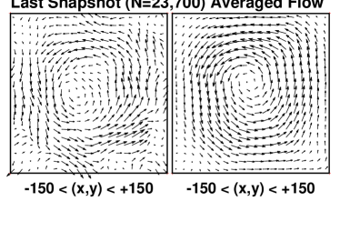
Particle escapes can be prevented by using a strong repulsive boundary potential to reflect any particle venturing “outside” the box. Figure 4 compares a time-averaged exposure of a typical molecular dynamics run with 23,700 particles to the final snapshot from the same simulation.

Figure 4: Simulation of Rayleigh-Bénard flow with molecular dynamics. A snapshot, using smooth-particle averages of the particle velocities, is at the left. Averages appear at the right.

Smooth Particle Applied Mechanics ( SPAMb8 ) is a macroscopic particle alternative to molecular dynamics. SPAM simulations are based on the continuum constitutive relations rather than atomistic interatomic forces. Hundreds of particles, rather than thousands, can generate rolls, the timestep is much larger, and individual snapshots do reproduce the stable roll structures quite well. SPAM defines local continuum averages by combining contributions from a few dozen nearby particles. All of these continuum properties, $\{\ \rho,u,e,P,Q,\ \dots\ \}$ are local averages from sums using a weight function like Lucy’s, which is shown in Figure 5 :

$$w(r<h)=(5/\pi h^{2})(1+3z)(1-z)^{3}\ ;\ z\equiv(r/h)\ .$$

Averages computed using this twice-differentiable weight function have two continuous spatial derivatives, enough for representing the righthand sides of the diffusive continuum equations with continuous functions.

Figure 5: Lucy’s weight function, normalized for two dimensions, $\int_{0}^{h}2\pi rw(r<h)dr\equiv 1$ .

Consider the simplest application of SPAM averaging, the definitions of the local densities and velocities in terms of smooth-particle weighted sums :

$$\rho(r)\equiv m\sum_{i}w(r-r_{i})\ ;\ \rho(r)u(r)\equiv m\sum_{i}w(r-r_{i})v_{i}\ .$$

These definitions satisfy the continuum continuity equation exactly! The variation of the density at a fixed location $r$ can be evaluated by the chain rule :

$$(\partial\rho/\partial t)_{r}=m\sum_{i}w^{\prime}v_{i}\cdot(r_{i}-r)/|r-r_{i}|\ .$$

Then notice that the gradient with respect to $r$ of the product $(\rho u)$ includes exactly the same terms, but with the opposite signs :

$$\nabla_{r}\cdot(\rho u)=m\sum_{i}w^{\prime}v_{i}\cdot(r-r_{i})/|r-r_{i}|\ .$$

Thus the SPAM version of the continuity equation ,

$$(\partial\rho/\partial t)\equiv-\nabla\cdot(\rho u)\longleftrightarrow\dot{\rho}=-\rho\nabla\cdot u\ ,$$

is an identity, independent of the form or range $h$ of the weight function $w(r<h)$ . This is not entirely a surprise as there is no ambiguity in the locations of the particles’ masses and momenta.

The pressure and energy are more complicated. The smooth-particle equation of motionb8 is antisymmetric in the particle indices. Thus that motion equation ,

$$\dot{v}_{i}\equiv-m\sum_{j}[\ (P/\rho^{2})_{i}+(P/\rho^{2})_{j}\ ]\cdot\nabla_{i}w(r_{i}-r_{j})\ ;$$

conserves linear momentum ( but not angular momentum ) exactly. Notice that whenever the pressure varies slowly in space the weight function plays the role of a repulsive potential with the strength of the interparticle “forces” proportional to the local pressure.

The gradients in SPAM are evaluated by taking derivatives of the corresponding sums. The temperature gradient, for example, is :

$$(\nabla T)_{i}\equiv m\sum_{j}(T_{j}-T_{i})w^{\prime}_{ij}[\ (r_{j}-r_{i})/(|r_{ij}|\rho_{ij})\ ]\ ;\ \rho_{ij}\equiv\sqrt{\rho_{i}\rho_{j}}\ {\rm or}\ (\rho_{i}+\rho_{j})/2\ .$$

Notice that two neighboring particles make no contribution to the temperature gradient if their temperatures match. With the gradients defined the pressure tensor and heat flux vectors can be evaluated for all the particles and used to advance the particle properties to the next time step :

$$\{\ \dot{r},\dot{v},\dot{e}\ \}\ \longrightarrow\ \{\ r,v,e\ \}$$

In all, the SPAM method averages involve about two dozen distinct particle properties. This computational effort is compensated by SPAM’s longer length and time scales.

In addition to providing an alternative approach to solving the continuum equations the SPAM averaging technique can be used to average molecular dynamics properties such as $P$ and $Q$. This approach is particularly valuable in shockwaves ( see Chapter 6 of Reference 7 ), where constitutive properties change on an atomistic distance scale. It would be interesting to compare the two sides of the continuum energy and motion equations and to use this comparison to optimize the choice of the weight function’s range $h$ .

The molecular dynamics results differ qualitatively from continuum results in their time symmetry, so that averaging offers a way of reducing this conflict. Time-dependent solutions offer a specially flexible technique for bringing the two approaches into better agreement. The weight functions also offer a way of carrying out the coarse graining which could be used to reduce the conflict between the microscopic and macroscopic forms of mechanics.

III.2 Eulerian Finite-Difference Methodb9

Straightforward centered-difference approximations to the continuum equations provide a useful approach to the Rayleigh-Bénard problem. Mareschal and his coworkers pointed out that an efficient numerical method can be based on square cells or zones, with the velocities and energies defined at the nodes and the densities defined in the cells. A small $10\times 10$ cell program written in this way would solve $3\times 11\times 11+10\times 10=463$ ordinary differential equations. The solution procedure follows a seven-step plan: [1] use linear interpolation and extrapolation near the boundaries to find the complete set of 484 nodal variables and 400 cell variables; [2] use centered differences to find $\nabla u$ and $\nabla T$ ; [3] use these gradients to obtain $P$ and $Q$ ; [4] evaluate $\nabla u:P$ and $\nabla\cdot Q$ ; [5] evaluate $(\partial\rho/\partial t)$ from the neighboring nodal values ; [6] evaluate $(\partial u/\partial t)$ from the pressure gradients and $(\partial e/\partial t)$ by summing the convective contributions and the work and heat; [7] use fourth-order Runge-Kutta integration to advance the 463 dependent variables to the next time step.

The Rayleigh-Bénard solutions – simple rollsb11 , periodic solutions, or chaos – can be observed in either two dimensions, where there are plenty of puzzles to solve, or three. Because simulation and visualization are simpler in two dimensions, while the challenges to understanding remain severe, we choose two dimensions. The critical Rayleigh Number of about 5000 corresponds to an eddy width which can easily be resolved with $8\times 8$ cells and a one-roll Reynolds number of order unity.

The Rayleigh number varies as $L^{4}$. Doubling the sidelength $L\rightarrow 2L$ with $g$ and the transport coefficients fixed changes ${\cal R}:5000\rightarrow 80000$ and increases the number of rolls to four. Desktop or laptop machines are quite capable of simulations with ${\cal R}=1\ 000\ 000$ , for which this simple-minded reasoning could lead us to expect about $(1000000/5000)^{1/4}\simeq 14$ rolls. In fact this doesn’t happen. See Figure 7 below. In two dimensions the energy flow is toward, rather than away from, large rolls. For ${\cal R}=800K$ [ $K$ indicates thousands ] and a $160\times 160$ mesh one finds occcasional deep minima in the time-dependent kinetic energy. These minima correspond to only two large rolls, as in the simple solutions without chaos, with ${\cal R}\simeq 10K$ . In three dimensions the chaotic flow is qualitatively different, and more complicated. Instead of whirling vortices one finds plumes ascending and descending, with mushroom shaped heads for large Prandtl numbers ( glycerin ) where viscosity dominates conductivityb1 .

Figure 6: Kinetic energy per cell (vertical at top and horizontal at bottom) from a simulation with ${\cal R}=t$. Notice, at the extreme left of the two plots, the reduction in the horizontal kinetic energy at the transition from one roll to two ( ${\cal R}\simeq 25K$ ) .

Figure 6 shows the variation of the kinetic energy per cell with the Rayleigh Number, where ${\cal R}=t\leq 700K$. The transitions go from one roll to two, and from two rolls to a time-periodic arrangement with perhaps four, which in turn gives rise to chaos. Our simple centered-finite-difference fixed-timestep code “blew up” at Rayleigh numbers of

$$\{\ 715K,\ 810K,\ 840K,\ 860K,\ 905K,\ 940K\ \}\ {\rm for}\ L=\{\ 16,\ 24,\ 32,\ 48,\ 64,\ 96\ \}\ .$$

Figure 6 suggests that chaos sets in around ${\cal R}=385K$ and gradually increases in strength until the algorithm becomes unstable for the chosen mesh.

The motion responds relatively quickly to perturbations. To demonstrate this we show in Figure 7 six snapshots from a $24\times 24$ simulation with all of the flow velocities instantaneously reversed from forward to backward at time 0, where the forward chaotic flow has three distinct rolls. By a time of 500 (a few dozen sound traversal times) the flow is back to normal, again with three rolls. But in the transformational process of discarding the time-reversed morphology the stabilizing flow acquires as many as seven rolls, in accord with the estimate that roughly $8\times 8$ cells are required to resolve a roll. The quick reduction in roll number as steady chaos is regained is again a symptom of the flow of energy from smaller to larger rolls in two dimensions.

Figure 7: Snapshots at time 0, 100, 200 (bottom row, left to right) and 300, 400, 500 (top row, left to right) starting with an instantaneously reversed chaotic flow with ${\cal R}=800\ 000$ .

Although there is no difficulty in simulating the motion on larger meshes even the modest 576-cell simulation of Figure 7 provides an excellent characterization of chaos. Characterizing chaos quantitatively entails evaluating Lyapunov exponents, the tendency of nearby trajectories to separate farther or to approach one another. The separation of a satellite trajectory from its reference has four component types :

$$\delta\equiv(\ \{\delta\rho\},\{\delta u_{x}\},\{\delta u_{y}\},\{\delta e\}\ )\ .$$

Keeping the separation constant by rescaling at every timestep gives the local exponent ,

$$\lambda_{i}(t)=\ln(|\ \delta_{\rm before}\ |/|\ \delta_{\rm after}\ |)/dt\ .$$

Figure 8: Separation between two strongly chaotic simulations. The fourth-order Runge-Kutta timestep is 0.05. Although four different sets of data (for $\rho,\ u,\ e$ subspaces as well as the complete space) are shown, here, the local Lyapunov exponents are scarcely distinguishable from one another.

In atomistic simulations it is well known that the largest Lyapunov exponent can be measured in configuration, momentum, or phase space, with identical longtime averagesb12 . In continuum simulations one would expect that the density, velocity, or energy subspaces could be used in this same way. By choosing particular mass, length, and time units any one of the three subspaces could be made to dominate the local Lyapunov exponent.

Figure 8 shows the exponential separation of a satellite trajectory from its reference trajectory, without rescaling, as measured in the density, velocity, energy, and complete state spaces of the flow. The similarity of the four curves is so complete that we don’t attempt to label them separatedly in the figure. Evidently, despite the changing morphology of the chaotic vortices, the underlying chaos ( at a Rayleigh Number of 800$K$ ) is quite steady. The research literature indicates that the Lyapunov spectrum in such two-dimensional flows is roughly linear, and corresponds to a strange attractor with only a few degrees of freedom, no doubt corresponding to the number of observed vortices.

The low dimensionality of two-dimensional turbulent chaos results from the tremendous dissipation inherent in the Navier-Stokes-Newton-Fourier model. If we evaluate the three “phase-space derivatives” which contribute to the continuum analog of Liouville’s particle Theorem :

$$(\partial\dot{\rho}/\partial\rho)\ ;\ (\partial\dot{u}/\partial u)\ ;\ (\partial\dot{e}/\partial e)\ ,$$

[ here the dots are time derivatives at fixed cells or nodes ] the velocity and energy derivatives give $-4(\eta/\rho)/(dx)^{2}$ and $-4\kappa/(dx)^{2}$ respectively while the density derivative vanishes. In the end only a few degrees of freedom exhibit chaos.

IV Conclusions and Suggestions for Research

Continuum mechanics can be studied with finite-difference ordinary differential equations, or with particle differential equations, resembling those used in molecular dynamics. The finite-difference approach is certainly the most efficient of these possibilities. The Rayleigh-Bénard problems exhibit a variety of flows, with interesting results at the level of a few hundred compuational cells. The relative stability of the flows and the characterization of the chaos are both interesting research areas. With the limited dimensionality of the chaotic flows’ attractors, estimating only a few Lyapunov exponents suffices to characterize Rayleigh-Bénard chaos. The loci of Lyapunov vectors’ instability is yet another source of fascinating questions and answers.

Though we have no space to discuss them here the useful smooth-particle technique for bridging together the particle and continuum methods suggests a variety of problems designed to reduce the discrepancies between the three types of numerical algorithm.

V Acknowledgments

We first learned about the Rayleigh-Bénard problem through a lecture by Jerry Gollub at Sitges some 25 years ago. That talk led to Ph D projects for Oyeon Kum and Vic Castillo at the University of California’s Davis/Livermore Campus’ “Teller Tech”. Their work continues to provide us with inspiration. We thank Denis Rapaport for helpful emails and Anton Krivtsov and Vitaly Kuzkin for encouraging our preparation of this lecture.

References

- (1) L. P. Kadanoff, “Turbulent Heat Flow: Structures and Scaling”, Physics Today 34-39 (August 2001).
- (2) N. T. Ouellette, “Turbulence in Two Dimensions”, Physics Today 68-69 (May 2012).
- (3) G. E. Karniadakis and S. A. Orszag, “Nodes, Modes, and Flow Codes”, Physics Today 34-42 (March 1993).
- (4) A. E. Deane and L. Sirovich, “A Computational Study of Rayleigh-Bénard Convection. Part 1. Rayleigh-Number Scaling [ and ] Part 2. Dimension Considerations”, Journal of Fluid Mechanics 222, 231-250 [ and ] 251-265 (1991).
- (5) R. H. Kraichnan and D. Montgomery, “Two-Dimensional Turbulence”, Reports on Progress in Physics 43, 547-619 (1980).
- (6) A. V. Getling, Rayleigh-Bénard Convection – Structures and Dynamics. (World Scientific, Singapore, 1998).
- (7) Wm. G. Hoover and Carol G. Hoover, Time Reversibility, Computer Simulation, Algorithms, and Chaos (Second Edition, World Scientific, Singapore, 2012) .
- (8) Wm. G. Hoover, Smooth Particle Applied Mechanics: the State of the Art, World Scientific, Singapore, 2006) .
- (9) A. Puhl, M. M. Mansour, and M. Mareschal, “Quantitative Comparison of Molecular Dynamics with Hydrodynamics in Rayleigh-Bénard Convection”, Physical Review A 40, 1999-2012 (1989).
- (10) D. C. Rapaport, “Hexagonal Convection Patterns in Atomistically Simulated Fluids”, Physical Review E 73, 025301R (2006).
- (11) V. M. Castillo, Wm. G. Hoover, and C. G. Hoover, “Coexisting Attractors in Compressible Rayleigh-Bénard Flow”, Physical Review E 55, 5546-5550 (1997).
- (12) S. D. Stoddard and J. Ford, “Numerical Experiments on the Stochastic Behavior of a Lennard-Jones Gas System”, Physical Review A 8, 1504-1512 (1973).