Adaptive fast multipole methods on the GPU

Abstract

We present a highly general implementation of fast multipole methods on graphics processing units (GPUs). Our two-dimensional double precision code features an asymmetric type of adaptive space discretization leading to a particularly elegant and flexible implementation. All steps of the multipole algorithm are efficiently performed on the GPU, including the initial phase which assembles the topological information of the input data. Through careful timing experiments we investigate the effects of the various peculiarities of the GPU architecture.

1 Introduction

We discuss in this paper implementation and performance issues for adaptive fast multipole methods (FMMs). Our concerns are focused on using modern high-throughput graphics processing units (GPUs) which have seen an increased popularity in Scientific Computing in recent years. This is mainly thanks to their high peak floating point performance and memory bandwidth, implying a theoretical performance which is an order of magnitude better than for CPUs (or even more). However, in practice for problems in Scientific Computing, the floating point peak performance can be difficult to realize since many such problems are bandwidth limited Vuduc et al. (2010). Although the GPU processor bandwidth is up to 4 times larger than that of the CPU, this is clearly not sufficient whenever the parallel speedup is (or could be) much larger than this. Moreover, according to the GPU computational model, the threads has to be run synchronously in a highly stringent manner. For these reasons, near optimal performance can generally only be expected for algorithms of predominantly data-parallel character.

Another difficulty with many algorithms in Scientific Computing is that the GPU off-chip bandwidth is comparably small such that the ability to mask this communication becomes very important Vuduc et al. (2010). Since the traditional form of many algorithms often involves intermediate steps for which the GPU architecture is sub-optimal, a fair degree of rethinking is usually necessary to obtain an efficient implementation.

Fast multipole methods appeared first in Greengard and Rokhlin (1987); Carrier et al. (1988) and have remained important computational tools for evaluating pairwise interactions of the type

$$\Phi(x_{i}) =\sum_{j=1,j\not=i}^{N}G(x_{i},x_{j}),\quad x_{i}\in\mathbf{R}^{D},\quad i=1\ldots N,$$ (1)

where $D\in\{2,3\}$. More generally, one may consider to evaluate

$$\Phi(y_{i}) =\sum_{j=1,x_{j}\not=y_{i}}^{N}G(y_{i},x_{j}),\quad i=1\ldots M,$$ (2)

where $\{y_{i}\}$ is a a set of evaluation points and $\{x_{j}\}$ a set of source points. In this paper we shall also conveniently use the terms potentials or simply particles to denote the set of sources $\{x_{j}\}$.

Although the direct evaluation of (1) has a complexity of $\mathcal{O}\left(N^{2}\right)$, the task is trivially parallelizable and can be performed much more efficiently using GPUs than CPUs. For sufficiently large $N$, however, tree-based codes in general and the FMM algorithm in particular become important alternatives. The practical complexity of FMMs scales linearly with the input data and, moreover, effective a priori error estimates are available. Parallel implementations are, however, often highly complicated and balancing efficiency with software complexity is not so straightforward Shanker and Huang (2007); Vikram et al. (2009).

In this paper we present a double precision GPU implementation of the FMM algorithm which is fully adaptive. Although adaptivity implies a more complex algorithm, this feature is critical in many important applications. Moreover, in our approach, all steps of the FMM algorithm are performed on the GPU, thereby reducing memory traffic to the host CPU.

Successful implementations of the FMM algorithm for GPUs have been reported previously Gumerov and Duraiswami (2008); Yokota and Barba (2011, 2012) under certain limitations. Specifically, with GPUs the performance of single precision algorithms is a factor of at least 2 times better than double precision (NVI, 2009, p. 11). In fact, for computationally intensive applications, this factor can reach as high as 8 times Wong et al. (2010), which implies that single precision speedups vis-à-vis CPU implementations can well be $>2$. It should be noted, however, that simpler tree-based methods than the FMM exist that offer a better performance at low tolerance (cf. Burtscher and Pingali (2011), (Griebel et al., 2007, Chap. 8.7)), and that the FMM is of interest mainly for higher accuracy demands.

In Section 2 we give an overview of our version of the adaptive FMM. The details of the GPU implementation are found in Section 3 and in a separate Section 4 we highlight the algorithmic changes that were made to the original serial code described in Engblom (2011). In Section 5 we examine in detail the speed-ups obtained when moving the various phases of the algorithm from the CPU to the GPU. We also reason about the results such that our findings may benefit others who try to port their codes to the GPU. Since the FMM has been judged to be one of the top 10 most important algorithms of the 20th century Cipra (2000), it is our hope that insights obtained here is of general value. A final concluding discussion around these matters is found in Section 6.

Availability of software

The code discussed in the paper is publicly available and the performance experiments reported here can be repeated through the Matlab-scripts we distribute. Refer to Section 6.1 for details.

2 Well-separated sets and adaptive multipole algorithms

In a nutshell, the FMM algorithm is a tree-based algorithm which produces a continuous representation of the potential field (2) from all source points in a finite domain. Initially, all potentials are placed in a single enclosing box at the zeroth level in the tree. The boxes are then successively split into child-boxes such that the number of points per box decreases with each level.

The version of FMM that we consider is described in Engblom (2011) and is organized around the requirement that boxes at the same level in the tree are either decoupled or strongly/weakly coupled. The type of coupling between the boxes follows from the $\theta$-criterion, which states that for two boxes with radii $r_{1}$ and $r_{2}$, whose centers are separated with distance $d$, the boxes are well-separated whenever

$$R+\theta r\leq\theta d,$$ (3)

where $R=\max\left\{r_{1},r_{2}\right\}$, $r=\min\left\{r_{1},r_{2}\right\}$, and $\theta\in(0,1)$ a parameter. In this paper we use the constant value $\theta=1/2$ which we have found to perform well in practice. At each level $l$ and for each box $b$, the set $S(p)$ of strongly coupled boxes of its parent box $p$ is examined; children of $S(p)$ that satisfy the $\theta$-criterion with respect to $b$ are allowed to become weakly coupled to $b$, otherwise they remain strongly coupled. Since a box is defined to be strongly connected to itself this rule defines the connectivity for the whole multipole tree. In Figure 1 an example of a multipole mesh and its associated connectivity pattern is displayed.

All boxes are equipped with an outgoing multipole expansion and an incoming local expansion. The multipole expansion is the expansion of all sources within the box around its center and is valid away from the box. To be concrete, in our two-dimensional implementation we use the traditional format of a $p$-term expansion in the complex plane,

$$M(z) =a_{0}\log(z-z_{0})+\sum_{j=1}^{p}\frac{a_{j}}{(z-z_{0})^{j}},$$ (4)

where $z_{0}$ is the center of the box. The local expansion is instead the expansion of sources far away from the box and can therefore be used to evaluate the contribution from these sources at all points within the box:

$$L(z) =\sum_{j=0}^{p}b_{j}(z-z_{0})^{j},$$ (5)

where again (5) is specific to a two-dimensional implementation.

The computational part of the FMM algorithm proceeds in an upward and a downward phase. During the first stage the multipole-to-multipole (M2M) shift from children to parent boxes recursively propagates and accumulates multipole expansions. In the second stage the important multipole-to-local (M2L) shift adds to the local expansions in all weakly coupled boxes which are then propagated downwards to children through the local-to-local shift (L2L). At the finest level, any remaining strong connections are evaluated through direct evaluation of (1) or (2). A simple optimization which was noted already in Carrier et al. (1988) is that, at the lowest level, strongly coupled boxes are checked with respect to the $\theta$-criterion (3), but with the roles of $r$ and $R$ interchanged. If found to be true, then the potentials in the larger box can be directly shifted into a local expansion in the smaller box, and the outgoing multipole expansion from the smaller can directly be evaluated within the larger box.

The algorithm so far has been described without particular assumptions on the multipole mesh itself. As noted in Engblom (2011), relying on asymmetric adaptivity when constructing the meshes makes a very convenient implementation possible. In particular, this construction avoids complicated cross-level communication and implies that the multipole tree is balanced, rendering the use of post-balancing algorithms Sundar et al. (2008) unnecessary. Also, the possibility to use a static layout of memory is particularly attractive when considering data-parallel implementations for which the benefits with adaptive meshes have been questioned Gumerov and Duraiswami (2008).

In this scheme, the child boxes are created by successively splitting the parent boxes close to the median value of the particle positions, causing all child boxes to have about the same number of particles. At each level, all boxes are split twice in succession, thus producing four times as many boxes for each new level. The resulting FMM tree is a pyramid rather than a general tree for which the depth may vary. The cost is that with a balanced tree, the communication stencil is variable. Additionally, it also prevents the use of certain symmetries in the multipole translations as described in Hrycak and Rokhlin (1998). To improve on the communication locality, the direction of the split is guided by the eccentricity of the box since the algorithm gains in efficiency when the boxes have equal width and height (the $\theta$-criterion is rotationally invariant).

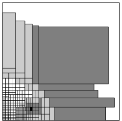
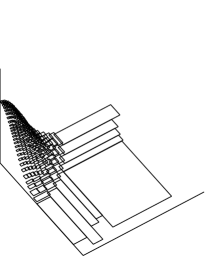
Figure 1: The adaptive mesh is constructed by recursively splitting boxes along the coordinate axes in such a way that the number of source points is very nearly the same in the four resulting boxes. (a) Here the boxes colored in light gray will interact via multipole-to-local shifts with the black box, that is, they satisfy the $\theta$-criterion ($\theta=1/2$). The boxes in dark gray are strongly connected to the black box and must be taken care of at the next level in the tree. (b) Same mesh as in (a), but visualized as a distribution by letting the height of each box be inversely proportional to its area. The source points in this example were sampled from a normal distribution.

The algorithmic complexity of the FMM has been discussed by many authors. Practical experiences Blelloch and Narlikar (1997), (Griebel et al., 2007, Chap. 8.7), (Gumerov and Duraiswami, 2004, Chap. 6.6.3), indicate that linear complexity in the number of source points is observed in most cases, but that simpler algorithms perform better in certain situations. Although it is possible to construct explicit distributions of points for which the FMM algorithm has a quadratic complexity Aluru (1996), this behavior is usually not observed in practical applications.

With $p$ terms used in both the multipole and the local expansions, we expect the serial computational complexity of our implementation to be proportional to $\theta^{-2}p^{2}\cdot N$, with $N$ the number of source points. This follows from assuming an asymptotically regular mesh such that $R\sim r$ in (3) and a total of on the order of $N$ boxes at the finest level. Then each of those $N$ boxes interact through M2L-interactions with about $\pi d^{2}\times N$ other boxes. From (3) we get $d\sim(1+\theta)/\theta\times r\sim(\sqrt{N}\theta)^{-1}$, and since the M2L-interaction is a linear mapping between $p$ coefficients this explains our stated estimate. This simple derivation assumes that the M2L-shift is the most expensive part of the algorithm. In practice, the cost of the direct evaluation of (1) may well match this part. From extensive experiments with the serial version of the algorithm, we have seen that it is usually possible to balance the algorithm in such a way that these two parts take roughly the same time.

With a given relative target tolerance $\operatorname{TOL}$, the analysis in Engblom (2011) implies $p\sim\log\operatorname{TOL}/\log\theta$, so that the total complexity can be expected to be on the order of $\theta^{-2}\log^{-2}\theta\cdot N\log^{2}\operatorname{TOL}$. We now proceed to discuss an implementation which distributes this work very efficiently on a GPU architecture.

3 GPU Implementation

The first major part of the adaptive fast multipole method is the topological phase which arranges the input into a hierarchical FMM mesh and determines the type of interactions to be performed. We discuss this part in Section 3.2. The second part is discussed in Section 3.3 and consists of the actual multipole evaluation algorithm with its upward and downward phases performing the required interactions in a systematic fashion.

To motivate some of our design choices, we choose to start with a brief discussion on the GPU hardware and the CUDA programming model (Compute Unified Device Architecture). The interested reader is referred to NVI (2012); Farber (2011) for further details.

3.1 Overview of the GPU architecture

Using CUDA terminology, the GPU consists of several multiprocessors (14 for the Tesla C2075), where each multiprocessor contains many CUDA cores (32 for the C2075). The CUDA execution model groups 32 threads together into a warp. All threads in the same warp execute the same instruction, but operate on different data; this is simply the GPU-version of the Single Instruction Multiple Data (SIMD)-model for parallel execution. Whenever two threads within the same warp need to execute different instructions, the operations become serialized.

To perform a calculation on the GPU, the CPU launches a kernel containing the code for the actual calculation. The threads on the GPU are grouped together into blocks, where the number of blocks as well as the number of threads per block is to be specified at each kernel launch (for performance reasons the number of threads per block is usually a multiple of the warp size). All threads within a block will be executed on the same multiprocessor and thread synchronization can only be performed efficiently between the threads of a single block. This synchronization is required whenever two threads write to the same memory address. Although for this purpose there are certain built-in atomic write operations, none of these support double precision for the Tesla C2075.

The GPU typically has access to its own global memory and all data has to be copied to this memory before being used. Further, each multiprocessor has a special fast shared memory, which can be used for the communication between threads within the same block (Farber, 2011, Chap. 5). For example, the C2075 has 48 kB of shared memory per multiprocessor for this purpose. Overuse of this memory limits the number of threads that can run simultaneously on a multiprocessor, which in turn has a negative effect on performance.

3.2 Topological phase

The topological phase consists of two parts, where the first part creates the boxes by partitioning the particles (we refer to this as “sorting”) and the second part determines the interactions between them (“connecting”).

The sorting algorithm successively partitions each box in two parts according to a chosen pivot point (Algorithm 3.1). The pivot element is obtained by first sorting 32 of the elements using a simple $\mathcal{O}\left(n^{2}\right)$ algorithm where each thread sorts a single point (32 elements was chosen to match the warp size). The pivot is then determined by interpolation of the current relative position in the active set of points so as to approximately land at the global median point (line 2, Algorithm 3.1).

Algorithm 3.1 (Partitioning with successive splits)

  

  Input: Unordered array consisting of $x$- or $y$-coordinates.

  Output: Array partitioned around its median coordinate.

1:  while size(array) $>$ 32 do

2:     determine_pivot_32()

3:     split_around_pivot()

4:     keep_part_containing_median()

5:  end while

6:  {the array now consists of $\leq$ 32 elements:}

7:  determine_median_32()

The split in line 3 uses a two-pass scheme, where each thread handles a small set of points to split. The threads start by counting the number of points smaller than the pivot. Then a global cumulative sum has to be calculated. Within a block, the method described in Harris et al. (2007) is used. For multiple blocks, atomic addition is used in between the blocks, thus allowing the split to be performed in a single kernel call (note that using atomic addition makes the code non-deterministic). Given the final cumulative sum, the threads can correctly insert their elements in the sorted array (second pass). After the split, only the part containing the median is kept for the next pass (line 4).

Algorithm 3.1 can be used to partition many boxes in a single kernel call using one block per box. If the number of boxes is low, it is desirable to use several blocks for each partitioning to better use the GPU cores. This requires communication between the blocks and the partitioning has to be performed with several kernel calls according to Algorithm 3.2. The splitting code is executed in a loop (lines 2 to 9) and a small amount of data transfer between the GPU and the CPU is required to determine the number of loops.

Algorithm 3.2 (Partitioning with successive splits, CPU part)

  

  Input: Unordered array consisting of $x$- or $y$-coordinates.

  Output: Array partitioned around its median coordinate.

1:  determine_split_direction()

2:  while $\max_{i}size(array_{i})>$ single_thread_limit do

3:     {executed in parallel:}

4:     for all splits do

5:        determine_pivot_32()

6:        partition_around_pivot()

7:        keep_part_containing_median()

8:     end for

9:  end while

10:  split_on_single_block()

Running the code using multiple blocks forces the code to run synchronized, with equal amount of splits in each partitioning. If one bad pivot is encountered, then this split takes much longer time than the others resulting in bad parallel efficiency. By contrast, a single block running does not force this synchronization and, additionally, allows for a better caching of the elements since they remain in the same kernel call all the time. For these reasons, Algorithm 3.2 switches to single block mode (line 10) when all splits contain a small enough number of points ($single\_thread\_limit=4096$ in the current implementation).

The second part of the topological phase determines the connectivity of the FMM mesh, that is, if the boxes should interact via near- or far-field interactions. This search is performed for each box independently and the parallelization one thread/box is used here. Each kernel call calculates the interactions of one full level of the FMM tree.

3.3 Computational part: the multipole algorithm

The computational part consists of all the multipole-related interactions, which include initialization (P2M), shift operators (M2M), (M2L), and (L2L), and local evaluation (L2P). Additionally, we also include the direct interaction in the near-field (P2P) in this floating point intensive phase of the FMM algorithm. During the computational part, no data transfer is necessary between the GPU and the host.

3.3.1 Multipole initialization

The initialization phase creates multipole expansions for each box via particle-to-multipole shifts (P2M). Since each source point gives a contribution to each coefficient $a_{j}$, using several threads per box requires intra-thread communication which in Algorithm 3.3 is accomplished by introducing a temporary matrix to store the coefficients.

Initially (line 5, Algorithm 3.3), one thread calculates the coefficients for one source particle (two threads if the number of particles is less than half the number of available threads). Then each thread calculates the sum for one coefficient (line 7). This procedure has to be repeated for a large number of coefficients, as it is desirable to have a small temporary matrix to limit the use of shared memory. The current implementation uses 64 threads per box (two warps) and takes 4 coefficients in each loop iteration (8 in the two threads/particle case).

The initialization also handles the special case where the particles are converted directly to local expansions via particle-to-local expansions (P2L). The principle for creating local expansions is the same as for the multipole expansions. All timings of this phase will include both P2M and P2L shifts.

Algorithm 3.3 (Multipole initialization)

  

  Input: Positions and strengths for source particles in a box.

  Output: Multipole coefficients $a_{i}$ for the box.

1:  {executed in parallel:}

2:  for all sources in box do

3:     load_one_source_per_thread()

4:     for $k=1$ to $p$ do

5:        temp_array := calc_N_cache_coefficients()

6:        synchronize_threads()

7:        $a_{k}$ := $a_{k}$ + sum(temp_array)

8:     end for

9:  end for

3.3.2 Upward pass

In the upward pass, the coefficients of each of four child boxes are repeatedly shifted to their parent’s coefficients via the M2M-shift. This is achieved using Algorithm 3.4 (a) which is similar to the one proposed in Liu (2009). Algorithm 3.4 (a) can be parallelized by allowing one thread to calculate one interaction, and at the end compute the sum over the four boxes (line 14, Algorithm 3.4). It should be noted that the multiplication in Algorithm 3.4 is a complex multiplication which is performed $\mathcal{O}\left(p^{2}\right)$ times. By introducing scaling, the algorithm can be modified to Algorithm 3.4 (b), which instead requires one complex division, $\mathcal{O}\left(p\right)$ complex multiplications and $\mathcal{O}\left(p^{2}\right)$ complex additions. The advantage of this modification in the GPU case is not the reduction of complex multiplications, but rather that the real and imaginary parts are independent. Hence two threads per shift can be used thus reducing the amount of shared memory per thread.

Algorithm 3.4 (Multipole to multipole translation)

  

  Input: Multipole coefficients $a_{j}$ of child box at position $z_{c}$.

  Output: Multipole coefficients $a_{j}$ of parent box at position $z_{p}$.

(a) Without scaling

1:  $r:=z_{c}-z_{p}$

2:  

3:  

4:  

5:  for $k=p$ downto 2 do

6:     for $j=k$ to $p$ do

7:        $a_{j}:=a_{j}+r\cdot a_{j-1}$

8:     end for

9:  end for

10:  for $j=1$ to $p$ do

11:     $a_{j}:=a_{j}-r^{j}\cdot a_{0}/j$

12:  end for

13:  {4 child boxes shift coefficients to the same parent:}

14:  $a:=$ sum_translations()

(b) With scaling

  $r:=z_{c}-z_{p}$

  for $j=1$ to $p$ do

     $a_{j}:=a_{j}/r^{j}$

  end for

  for $k=p$ downto 2 do

     for $j=k$ to $p$ do

        $a_{j}:=a_{j}+a_{j-1}$

     end for

  end for

  for $j=1$ to $p$ do

     $a_{j}:=(a_{j}-a_{0}/j)\cdot r^{j}$

  end for

  

  

  $a:=$ sum_translations()

3.3.3 Downward pass

The downward pass consists of two parts, the translation of multipole expansions to local expansions (M2L), and the translation of local expansions to the children of a box (L2L). The translation of local expansions to the children is very similar to the M2M-shift discussed previously, and can be achieved with the scheme in Algorithm 3.5 (b). This shift is slightly simpler on the GPU since there is no need to sum the coefficients at the end, but instead requires more memory accesses as the calculated local coefficients must be added to already existing values.

Algorithm 3.5 (Local to local translation)

  

  Input: Local coefficients $b_{j}$ of parent box at position $z_{p}$.

  Output: Local coefficients $b_{j}$ of child box at position $z_{c}$.

1:  $r:=z_{p}-z_{c}$

2:  for $j=1$ to $p$ do

3:     $b_{j}:=b_{j}\cdot r^{j}$

4:  end for

5:  for $k=0$ to $p$ do

6:     for $j=p-k$ to $p-1$ do

7:        $b_{j}:=b_{j}-b_{j+1}$

8:     end for

9:  end for

10:  for $j=1$ to $p$ do

11:     $b_{j}:=b_{j}/r^{j}$

12:  end for

The translation of multipole expansions to local expansions is the most time consuming part of the downward pass. The individual shifts can be performed with a combination of the reduction scheme in the M2M translation and the L2L translation, see Algorithm 3.6. Again, this implementation allows for two dedicated threads for each shift. We have not seen this algorithm described elsewhere.

Algorithm 3.6 (Multipole to local translation)

  

  Input: Multipole coefficients $a_{j}$ of box at position $z_{i}$.

  Output: Local coefficients $b_{j}$ of box at position $z_{o}$.

1:  $r:=z_{o}-z_{i}$

2:  for $j=1$ to $p$ do

3:     $b_{j-1}:=a_{j}/r^{j}\cdot(-1)^{j}$

4:  end for

5:  $b_{p}:=0$

6:  for $k=2$ to $p$ do

7:     for $j=p-k$ to $p-1$ do

8:        $b_{j}:=b_{j}-b_{j+1}$

9:     end for

10:  end for

11:  for $k=p$ downto 1 do

12:     for $j=k$ to $p$ do

13:        $b_{j}:=b_{j}+b_{j-1}$

14:     end for

15:  end for

16:  $b_{0}:=b_{0}-a_{0}\cdot\log(r)$

17:  for $j=1$ to $p$ do

18:     $b_{j}:=(b_{j}-a_{0}/j)/r^{j}$

19:  end for

20:  $b:=$ sum_translations()

With the chosen adaptive scheme, the number of shifts per box varies. Since our GPU does not support atomic addition in double precision, one block has to handle all shifts of one box in order to perform this operation in one kernel call. As the number of translations is not always a multiple of 16 (the number of translations per loop if 32 threads/block is used), this can result in idle threads. One can partially compensate for this by giving one block the ability to operate on two boxes in the same loop.

As the M2L translations are performed within a single level of the multipole tree, all translations can be performed in a single kernel call. This is in contrast to the M2M- and L2L translations, which both require one kernel call per level.

3.3.4 Local evaluation

The local evaluation (L2P) is scheduled in parallel by using one block to calculate the interactions of one box. Moreover, one thread calculates the interactions of one evaluation point from the local coefficients of the box. This operation requires no thread communication and can be performed in the same way as for the CPU. The local evaluation uses 64 threads/block.

This phase will also include the special case where the evaluation is performed directly through the multipole expansion (M2P). This operation is performed in a similar way as for the L2P evaluation. All timings of this phase therefore include both L2P- and M2P evaluations.

3.3.5 Near-field evaluation

In the near-field evaluation (P2P), the contribution $F$ from all boxes within the near-field of a box should be calculated at all evaluation points of the box. Similar to the M2L translations, the number of boxes in the near-field varies due to the adaptivity.

Algorithm 3.7 (Direct evaluation between boxes)

  

  Input: Positions and strengths of particles in the near field.

  Output: The contribution $F$ of the particles in the near field.

1:  {executed in parallel:}

2:  load_evaluation_point_positions() {one per thread}

3:  for all interaction boxes do

4:     cache_interaction_positions()

5:     if  cache_is_full or all_positions_loaded then

6:        for all elements in cache do

7:           $F$ := $F$ + add_pairwise_interaction()

8:        end for

9:     end if

10:  end for

The GPU implementation uses one block per box and one to four threads per evaluation point (depending on the number of evaluation points compared to the number of threads). The interaction is calculated according to Algorithm 3.7, where the source points are loaded into a cache in shared memory (line 4) and when the cache is full, the interactions are calculated (line 7). This part uses 64 threads per block and a suitable cache size is to use the same size as the number of threads.

4 Differences between the CPU and GPU implementations

In this section we highlight the main differences between the two versions of the code. A point to note is that when we compare speed-up with respect to the CPU-code in Section 5, we have taken care in implementing several optimizations which are CPU-specific.

4.1 Topological phase

When sorting, the GPU implementation is based on sorting 32 element arrays for choosing a pivot element. This design was made to achieve a better use of the CUDA cores and, in the multiple block/partitioning case, to make all partitionings behave more similar to each other. The single-threaded CPU version uses the median-of-three procedure for choosing the pivot element, which is often used in the well-known algorithm quicksort (Sedgewick, 1990, Chap. 9). An advantage with this method compared to the GPU algorithm is that it is in-place and hence that there is no need for temporary storage.

4.2 Computational part

The direct evaluation can use symmetry on the CPU if the evaluation points are the same as the source points since the direct interaction is symmetric. Using this symmetry, the run time of the direct interaction can be reduced by almost a factor of two in the CPU version. This is not implemented on the GPU as it would require atomic memory operations to store the results (which is not available for double precision on our GPU).

The operations M2M, P2P, P2M, and M2P are all in principle the same in both versions of the code. For the M2L shift, the symmetry of the $\theta$-criterion (3) can be used in the scaling phases on the CPU (lines 2–4 and 17–19 in Algorithm 3.6), while in the GPU version, the two shifts are handled by different blocks, making communication unpractical. Another difference is that the scaling vector is saved in memory from the pre-scaling part to the post-scaling part after the principal shift operator. This was intentionally omitted from the GPU version as the extra use of shared memory decreased the number of active blocks on each multiprocessor, and this in turn reduced performance.

4.3 Symmetry and connectivity

The CPU implementation uses symmetry throughout the multipole algorithm. With symmetry, it is only required to create one-directional interaction lists when determining the connectivity.

As the GPU implementation does not rely on symmetry when evaluating, it is beneficial to create directed interaction lists. This causes twice the work and twice the memory usage (for the connectivity lists). However, the time required to determine the connectivity is quite small ($\sim$ 1%, see Table 1).

4.4 Further notes on the CPU implementation

The current CPU implementation is a single threaded version. Other research Cruz et al. (2011); Vuduc et al. (2010) has shown that good parallel efficiency can be obtained for a multicore version (e.g. 85% parallel efficiency on 64 processors). However, the work in Cruz et al. (2011) does not appear to use the symmetry in the compared direct evaluation.

In order to achieve a highly efficient CPU implementation, as suggested also by others Yokota and Barba (2012); Tanikawa et al. (2012), the multipole evaluation part was written using SSE intrinsics. Using these constructs means that two double precision operations can be performed as one single operation. The direct- and multipole evaluation, as well as the multipole initialization all use this optimization, where two points are thus handled simultaneously. Additionally, all shift operators also rely on SSE intrinsics in their implementation.

4.5 Double versus single precision

The entire algorithm is written in double precision for both the CPU and the GPU. Using single precision would be significantly faster, both on the CPU (as SSE could operate on 4 floats instead of 2 doubles) and on the GPU (where the performance difference appears to vary depending on the mathematical expression Wong et al. (2010)). It is likely that higher speedups could be obtained with a single precision code, but it would also seriously limit the applicability of the algorithm. With our approach identical accuracy is obtained from the two codes.

5 Performance

This section compares the CPU and GPU codes performance-wise. The simulations were performed on a Linux Ubuntu 10.10-system with an Intel Xeon 6c W3680 3.33 GHz CPU and a Nvidia Tesla C2075 GPU. The compilers were GCC 4.4.5 and CUDA 4.0. For all comparisons of individual parts, the sorting was performed on the CPU to ensure identical multipole trees (the GPU sorting algorithm is non-deterministic). All timings have been handled using the timing functionality of the GPU. The total time includes the time to copy data between the host and the GPU, while the time of the individual parts does not include this. All simulations were performed a large number of times such that the error in the mean when regarded as an estimator to the expected value was negligible. Overall we found that the measured times displayed a surprisingly small spread with usually a standard deviation which was only some small fraction of the measured value itself.

All performance experiments were conducted using the harmonic potential,

$$G(z_{i},z_{j}) \equiv\frac{\Gamma_{j}}{z_{j}-z_{i}},$$ (6)

in (1) and hence $a_{0}=0$ in (4). Moreover, in Sections 5.1 through 5.3, all simulations were performed using randomly chosen source points, homogeneously distributed in the unit square.

We remark again that the performance experiments reported here can be repeated using the scripts distributed with the code itself, see Section 6.1.

5.1 Calibration

From the perspective of performance, the most critical parameter is the number of levels in the multipole tree. Adding one extra level increases the number of boxes at the finest level in the tree by four. Assuming that each box connects to approximately the same number of boxes at each level, the total number of pairwise interactions therefore decrease with a factor of about 4. The initialization and multipole evaluation require the same amount of operations, but will operate on an increasing number of boxes, thus increasing the memory accesses. For all shift operations, one additional level implies about a threefold increase of the total number of interactions and the same applies for the determination of the connectivity information. For the sorting, each level requires about the same amount of work, but handling many small boxes easily causes additional overhead.

It is expected that the CPU code will follow this scaling quite well, while for the GPU, where several threads should run synchronously, this is certainly not always the case. As an example, L2P operates by letting one thread handle the interaction of one source point, P2M can use up to two threads, and P2P can use up to four threads/point (all these use 64 threads/block). On the tested Tesla C2075 system, this means that the local evaluation of a box containing 1 evaluation point takes the same amount of time as a box containing 64 evaluation points (on a Geforce GTX 480 system, this only applies to up to 32 evaluation points which is the warp size here). This shows the sensitivity of the GPU implementation with respect to the number of points in each box.

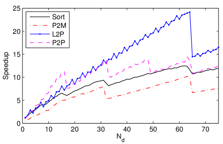
Figure 2: Speedup of the individual parts of the GPU-implementation as a function of the number of sources per box $N_{d}$. Here the total number of sources varies between $2^{16}$ and $75\times 2^{16}$.

In Figure 2, the GPU speedup as a function of the number of sources per box is studied. Within this range, the shift operators and the connectivity mainly depend on the number of levels and therefore obtain constant speedups (hence we omit them). All parts that depend on the number of particles in each box obtain higher speedups for larger number of particles per box. This is expected, since it is easier to get a good GPU load for larger systems. There is also a performance decrease when the number of particles increases above 32, 64, and so on, that is, at multiples of the warp size. The direct evaluation additionally shows a performance decrease directly after each multiple of 16, which is due to the fact that the algorithm can use 4 threads per particle.

The small high frequency oscillations seen in the speedup of L2P and P2P originates from the CPU algorithm, and is due to the use of SSE instructions which makes the CPU code more efficient for an even number of sources per box.

It should be noted again that the direct evaluation and connectivity both make use of symmetry in the CPU version. This means that the speedup would be significantly higher (almost a factor 2) if the CPU version did not rely on this symmetry.

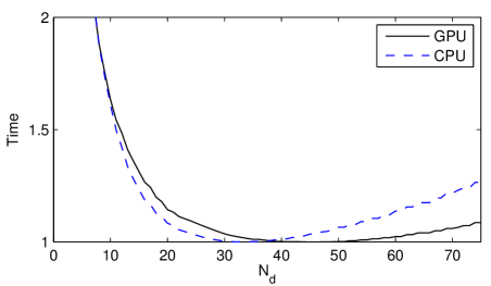
Figure 3: Time as a function of the number of sources per box $N_{d}$ for the CPU and the GPU implementation, both normalized so that the fastest time $\equiv 1$.

As adding one extra level reduces the computational time of the direct interaction, but increases the time requirement for most other parts, it is necessary to find the best range of particles per box. The number of levels $N_{l}$ is calculated according to

$$N_{l} =\left\lceil 0.5\log_{2}\left(\frac{5}{8}\frac{N}{N_{d}}\right)\right\rceil,$$ (7)

where $N$ is the number of particles and $N_{d}$ is the desired number of particles per box. This parameter choice was studied for 150 simulations with different number of particles (from $1\times 10^{4}$ to $2\times 10^{6}$). The result (normalized against the lowest time on each platform) is found in Figure 3, showing that a value around 45 is best for the GPU, while 35 is best for the CPU. Even though the GPU has poor speedup for low number of particles, it still scales better than the CPU in this case. The reason is that with low values of $N_{d},$ the multipole shifts dominate the computational time. This simulation was performed with 17 multipole coefficients, giving a tolerance of approximately $1\times 10^{-6}$. The tolerance is here and below understood as

$$\operatorname{TOL} =\left\|\frac{\Phi_{FMM}-\Phi_{exact}}{\Phi_{exact}}\right\|_{\infty}$$ (8)

where $\Phi_{exact}$ is the exact potential and $\Phi_{FMM}$ is the FMM result.

Part	Time	Part	Time
P2P	43 %	Connect	1 %
Sort	30 %	M2M	$<1$ %
M2L	11 %	L2L	$<1$ %
P2M	5 %
L2P	2 %	Other	8 %

Table 1: Time distribution of the GPU algorithm. The most expensive part in the case studied here is the direct evaluation (P2P), followed by sorting and M2L translations. The field “other” contains all data transfers between the host and the GPU.

For the optimal value 45 of $N_{d}$, the time distribution of the different parts of the algorithm is given in Table 1 for $N=45\times 2^{16}$, which gives 45 sources in each box at the finest level of the FMM tree. According to (7), using $N_{d}=45$ gives 8 levels for $N\in(18\times 2^{16},72\times 2^{16}]$. Within this interval, the time of P2P relative to the total time varies between 25% to 55%. It is particularly interesting to note in Table 1 that the sorting dominates by a factor of about 3 over the usually very demanding M2L-operation.

5.2 Shift operators

The performance of the sorting and direct evaluation depends on the number of sources per box and the number of levels while the connectivity to a first approximation only depends on the number of levels. The rest of the operators also depend on the number of multipole coefficients (the number of multipole coefficients determine the error in the algorithm). Multipole initialization and evaluation depends linearly on the number of coefficients, while the shift operators have two linear parts (pre- and post-scaling) and one quadratic part (the actual shift). In the GPU case, all accesses to global memory are included in the linear parts while all data is kept in shared memory during the shift. A higher number of coefficients increases the use of shared memory and fewer shift operations can therefore be performed in parallel. The speedup as a function of number of coefficients is plotted in Figure 4, where the simulation was performed on $10^{6}$ particles with $N_{d}=45$. The decrease in speedup due to lack of shared memory can be seen quite clearly, e.g. at 42 coefficients for the M2L-shift, where one block less (3 in total) can operate on the same multiprocessor.

The difference in speedup for L2P at low number of coefficients is likely due to overhead, since these values stabilize at high enough number of coefficients.

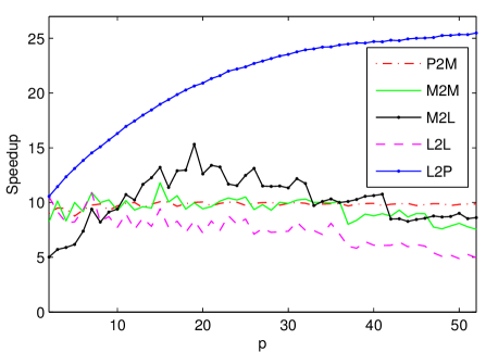
Figure 4: Speedup as a function of the number of multipole coefficients $p$.

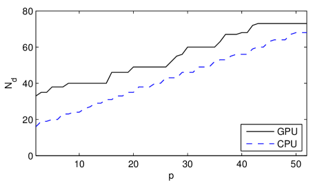
Figure 5: Optimal value of $N_{d}$ as a function of the number of multipole coefficients $p$.

Considering that the time required for the shift operators increases with increasing number of coefficients, the optimal value for $N_{d}$ changes as well. Figure 5 shows that the optimal number for $N_{d}$ increases approximately linearly with increasing number of coefficients.

5.3 Break-even

If the number of sources is low enough, it may be faster to use a direct summation instead of the fast multipole method. In Figure 6, the speed of the entire algorithm is compared with the speed of direct summation for both the CPU and the GPU implementation. The speedup of the GPU code increases with the number of particles since more source points provide a better load for the GPU. Looking at the direct summation times, the GPU scales linearly in the beginning where the number of working cores is still increasing, and later scales quadratically as the cores become fully occupied. Since a double sum is easily performed in parallel and is not memory bandwidth dominated the direct evaluation provides a good estimate of the maximum speedup that can be achieved with the GPU. Recall, however, that symmetry is used in the CPU implementation, which almost speeds up the calculation with a factor of 2. Figure 6 shows that it is more beneficial to use the FMM algorithm if the number of points exceeds about 3500 on the GPU. This result compares favorably with that reported by others Yokota and Barba (2011). For large $N$, the speedup of the direct interaction is higher than that of the FMM (15 compared to about 11, see Figure 7). Again, one should note that the CPU version uses symmetry here. For simulations where the source points and evaluation points are separate, the speedup is about 30 for the direct evaluation and 15 for the FMM. The lower increase in speedup for the FMM is due to the fact that only the P2P-evaluation of the algorithm uses this symmetry (compare Table 1).

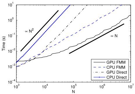
Figure 6: Total time of the algorithm as a function of the number of sources $N$. For the FMM-algorithm, the simulation was performed with $p=17$, implying a tolerance of about $10^{-6}$.

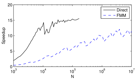
Figure 7: Speedup as a function of the number of sources $N$.

Comparing the individual parts (Figure 8), the M2L- and P2P-shifts quite rapidly obtain high speedups, while the sorting requires quite a large number of points. The poor values for M2M and L2L at low number of particles are due to the fact that few shifts are performed at the lower levels, causing many idle GPU cores. The situation is the same for the connectivity. As these algorithms have to be performed one level at a time, the low performance of the shifts high up in the multipole tree decreases the performance of the entire step. Consequently, the speedup increases with an increasing number of source points. The oscillating behavior of the multipole initialization and evaluation is related to the number of particles in each box (compare with Figure 2).

The code has been tested both on the Tesla platform used for the above figures, and on a Geforce GTX 480 platform (which has 480 cores, compared to 448 for the Tesla card). The total run-time is approximately the same on both platforms. Notable differences are that the P2P interaction is faster on the Tesla if $N_{d}$ is high, and in the simulation in Table 1, the GTX 480 card required 30% longer time than the Tesla card. On the other hand, the Tesla card required 25% longer time than the GTX 480 for the sorting (which is limited by memory access, rather than double precision math). The shift operators were approximately equally fast on both systems. The overall result is that the optimal value for $N_{d}$ is lower for the GTX 480 card (35 instead of 45) for a total running time which was approximately the same. This shows that the much cheaper GTX 480 gaming card is a perfectly reasonable option for this implementation of the fast multipole method, despite the fact that it is written in double precision.

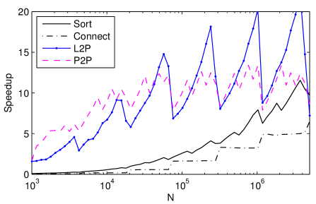
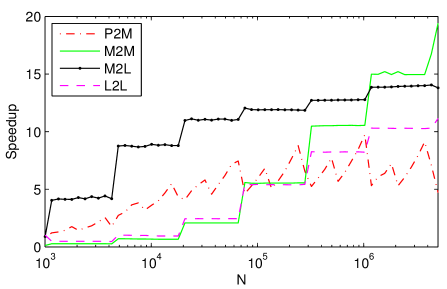
Figure 8: Speedup of individual parts as a function of the number of sources.

5.4 Benefits of adaptivity

As a final computational experiment we investigated the performance of the adaptivity by using different point distributions. Under a relative tolerance of $10^{-6}$ ($p=17$ in (4) and (5)) we measured the evaluation time for increasing number of points sampled from three very different distributions. As shown in Figure 9, the code is robust under highly non-uniform inputs and scales well at least up to some 10 million source points.

When the distribution of particles is increasingly non-uniform, more boxes will be in each others near-field resulting in more direct interactions. This is tested in Figure 10 for the two non-uniform distributions from Figure 9. Both the CPU- and GPU timings have been normalized to the time of a homogeneous distribution. The results indicate that the decrease in performance for highly non-uniform distributions is less for the GPU version than for the CPU version. From the timings of the individual parts, it is seen that almost all the increase in computational time originates from the P2P-shift. The speedup for all time consuming individual parts is relatively constant with respect to the degree of non-uniformity (e.g. the parameter $\sigma$ in Figure 10) and the reason the GPU code handles a highly non-uniform distribution better is simply because the P2P evaluation has a higher speedup than the overall code.

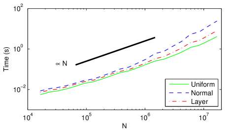
Figure 9: Performance of the code when evaluating the harmonic potential for three different distributions of points. The source points were (i) uniformly distributed in $[0,1]\times[0,1]$, (ii) normally distributed with variance $1/100$, and (iii) distributed in a ‘layer’ where the $x$-coordinate is uniform, and the $y$-coordinate is again $N(0,1/100)$-distributed. For the purpose of comparison, all distributions were rejected to fit exactly within the unit square. The FMM mesh for case (ii) is shown in Figure 1.

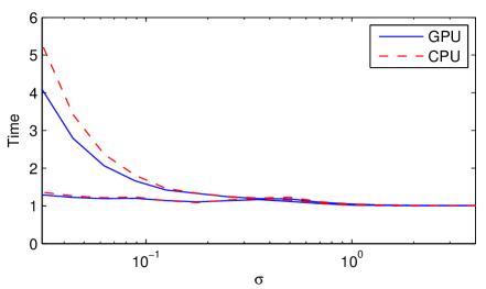
Figure 10: Robustness of adaptivity. Time for two different non-uniform distributions normalized with respect to a uniform distribution of points. The top two graphs are for the normal distribution of sources, while the lower two graphs are for the ‘layer’ distribution. See text for further details.

6 Conclusions

We have demonstrated that all parts of the adaptive fast multipole algorithm can be efficiently implemented on a GPU platform in double precision. Overall, we obtain a speedup of about a factor of 11 compared to a highly optimized (including SSE intrinsics), albeit serial, CPU-implementation. This factor can be compared with the speedup of about 15 which we obtain obtained for the direct $N$-body evaluation, a task for which GPUs are generally understood to be well suited Rapaport (2011) (see Figure 7).

In our implementation, all parts of the algorithm achieve speedups in about the same order of magnitude. Generally, we obtain a higher speedup whenever the boxes contain some 20–25% more particles than the CPU version (see Figures 5 and 8). Given the data-parallel signature of this particular operation, this result is quite expected. Another noteworthy result is that our version of the GPU FMM is faster than the direct $N$-body evaluation at around $N=3500$ source points, see Figure 6. Our tests also show that the asymmetric adaptivity works at least as well on the GPU as on the CPU, and that in some cases it even performs better.

When it comes to coding complexity it is not so straightforward to present actual figures, but some observations at least deserve to be mentioned. The topological phase was by far the most difficult part to implement on the GPU. In fact, the number of lines of codes approximately quadrupled when transferring this operation. We remark also that the topological phase performs rather well on the GPU, an observation which can be attributed to its comparably high internal bandwidth. Thus, there is a performance/software complexity issue here, and striking the right balance is not easy.

By contrast, the easiest part to transfer was the direct evaluation (P2P), where, due to SSE-intrinsics, the CPU-code is in fact about twice the size than the corresponding CUDA-implementation.

These observations as well as our experimental results, suggest that a balanced implementation, where parts of the algorithm are off-loaded to the GPU while the remaining parts are parallelized over the CPU-cores, would be a reasonable compromise. This has also been noted by others Burtscher and Pingali (2011) and is ongoing research.

6.1 Reproducibility

Our implementation as described in this paper is available for download via the second author’s web-page. The code compiles both in a serial CPU-version and in a GPU-specific version and comes with a convenient Matlab mex-interface. Along with the code, automatic Matlab-scripts that repeat the numerical experiments presented here are also distributed.

References

- Aluru (1996) S. Aluru. Greengard’s -body algorithm is not order . SIAM J. Sci. Comput., 17(3):773–776, 1996. doi:10.1137/S1064827593272031.
- Blelloch and Narlikar (1997) G. Blelloch and G. Narlikar. A practical comparison of -body algorithms. In Parallel Algorithms, volume 30 of Series in Discrete Mathematics and Theoretical Computer Science, 1997.
- Burtscher and Pingali (2011) M. Burtscher and K. Pingali. An efficient CUDA implementation of the tree-based Barnes Hut -body algorithm. In W.-M. Hwu, editor, GPU Computing Gems Emerald Edition, chapter 6, pages 75–92. Morgan Kaufmann/Elsevier, 2011.
- Carrier et al. (1988) J. Carrier, L. Greengard, and V. Rokhlin. A fast adaptive multipole algorithm for particle simulations. SIAM J. Sci. Stat. Comput., 9(4):669–686, 1988. doi:10.1137/0909044.
- Cipra (2000) B. A. Cipra. The best of the 20th century: Editors name top 10 algorithms. SIAM News, 33(4), 2000.
- Cruz et al. (2011) F. A. Cruz, M. G. Knepley, and L. A. Barba. Petfmm-a dynamically load-balancing parallel fast multipole library. Internat. J. Numer. Methods Engrg., 85(4):403–428, 2011. doi:10.1002/nme.2972.
- Engblom (2011) S. Engblom. On well-separated sets and fast multipole methods. Appl. Numer. Math., 61(10):1096–1102, 2011. doi:10.1016/j.apnum.2011.06.011.
- Farber (2011) R. Farber. CUDA Application Design and Development. Morgan Kaufmann Publishers Inc., San Francisco, CA, USA, 1st edition, 2011.
- Greengard and Rokhlin (1987) L. Greengard and V. Rokhlin. A fast algorithm for particle simulations. J. Comput. Phys., 73(2):325–348, 1987. doi:10.1016/0021-9991(87)90140-9.
- Griebel et al. (2007) M. Griebel, S. Knapek, and G. Zumbusch. Numerical Simulation in Molecular Dynamics, volume 5 of Texts in Computational Science and Engineering. Springer Verlag, Berlin, 2007.
- Gumerov and Duraiswami (2004) N. A. Gumerov and R. Duraiswami. Fast multipole methods for the Helmholtz equation in three dimensions. Elsevier Series in Electromagnetism. Elsevier, Oxford, 2004.
- Gumerov and Duraiswami (2008) N. A. Gumerov and R. Duraiswami. Fast multipole methods on graphics processors. J. Comput. Phys., 227(18):8290–8313, 2008. doi:10.1016/j.jcp.2008.05.023.
- Harris et al. (2007) M. Harris, S. Sengupta, and J. D. Owens. Parallel prefix sum (scan) with CUDA. In H. Nguyen, editor, GPU Gems 3, chapter 39, pages 851–876. Addison Wesley, 2007.
- Hrycak and Rokhlin (1998) T. Hrycak and V. Rokhlin. An improved fast multipole algorithm for potential fields. SIAM J. Sci. Comput., 19(6):1804–1826, 1998. doi:10.1137/S106482759630989X.
- Liu (2009) Y. Liu. Fast Multipole Boundary Element Method: Theory and Applications in Engineering. Cambridge University Press, Cambridge, 2009.
- NVI (2009) NVIDIA’s Next Generation CUDA Compute Architecture: Fermi. NVIDIA, 2009. Available at http://www.nvidia.com/content/PDF/fermi_white_papers/NVIDIA_Fermi_Compute_Architecture_Whitepaper.pdf.
- NVI (2012) CUDA C Programming Guide. NVIDIA, 2012. Version 4.2. Available at http://developer.download.nvidia.com/compute/DevZone/docs/html/C/doc/CUDA_C_Programming_Guide.pdf.
- Rapaport (2011) D. C. Rapaport. Enhanced molecular dynamics performance with a programmable graphics processor. Comput. Phys. Comm., 182(4):926–934, 2011. doi:10.1016/j.cpc.2010.12.029.
- Sedgewick (1990) R. Sedgewick. Algorithms in C. Addison-Wesley Series in Computer Science. Addison-Wesley, Reading, MA, 1990.
- Shanker and Huang (2007) B. Shanker and H. Huang. Accelerated Cartesian expansions - a fast method for computing of potentials of the form for all real . J. Comput. Phys., 226(1):732–753, 2007. doi:10.1016/j.jcp.2007.04.033.
- Sundar et al. (2008) H. Sundar, R. S. Sampath, and G. Biros. Bottom-up construction and 2:1 balance refinement of linear octrees in parallel. SIAM J. Sci. Comput., 30(5):2675–2708, 2008. doi:10.1137/070681727.
- Tanikawa et al. (2012) A. Tanikawa, K. Yoshikawa, T. Okamoto, and K. Nitadori. N-body simulation for self-gravitating collisional systems with a new simd instruction set extension to the x86 architecture, advanced vector extensions. New Astron., 17(2):82–92, 2012. doi:10.1016/j.newast.2011.07.001.
- Vikram et al. (2009) M. Vikram, A. Baczewzki, B. Shanker, and S. Aluru. Parallel accelerated Cartesian expansions for particle dynamics simulations. In Proceedings of the 2009 IEEE International Parallel and Distributed Processing Symposium, pages 1–11, 2009. doi:10.1109/IPDPS.2009.5161038.
- Vuduc et al. (2010) R. Vuduc, A. Chandramowlishwaran, J. Choi, M. Guney, and A. Shringarpure. On the limits of GPU acceleration. In Proceedings of the 2nd USENIX conference on Hot topics in parallelism, HotPar’10, Berkeley, CA, USA, 2010. USENIX Association.
- Wong et al. (2010) H. Wong, M.-M. Papadopoulou, M. Sadooghi-Alvandi, and A. Moshovos. Demystifying GPU microarchitecture through microbenchmarking. In 2010 IEEE International Symposium on Performance Analysis of Systems Software (ISPASS), pages 235–246, 2010. doi:10.1109/ISPASS.2010.5452013.
- Yokota and Barba (2011) R. Yokota and L. Barba. Treecode and fast multipole method for N-body simulation with CUDA. In W.-M. Hwu, editor, GPU Computing Gems Emerald Edition, chapter 9, pages 113–132. Morgan Kaufmann/Elsevier, 2011.
- Yokota and Barba (2012) R. Yokota and L. Barba. A tuned and scalable Fast Multipole Method as a preeminent algorithm for exascale systems. Int. J. High-perf. Comput. Appl., 2012. doi:10.1177/1094342011429952.