Theoretical study of magnetic domain walls through a cobalt nanocontact

Abstract

To calculate the magnetic ground state of nanoparticles we present a self-consistent first principles method in terms of a fully relativistic embedded cluster multiple scattering Green’s function technique. Based on the derivatives of the band energy, a Newton-Raphson algorithm is used to find the ground state configuration. The method is applied to a cobalt nanocontact that turned out to show a cycloidal domain wall configuration between oppositely magnetized leads. We found that a wall of cycloidal spin-structure is about 30 meV lower in energy than the one of helical spin-structure. A detailed analysis revealed that the uniaxial on-site anisotropy of the central atom is mainly responsible to this energy difference. This high uniaxial anisotropy energy is accompanied by a huge enhancement and anisotropy of the orbital magnetic moment of the central atom. By varying the magnetic orientation at the central atom, we identified the term related to exchange couplings (Weiss-field term), various on-site anisotropy terms, and also those due to higher order spin-interactions.

I Introduction

As magnetic storage devices approach a physical limit of a single atom, the investigation of nanoclusters has become one of the most important subjects in magnetism. Recent developments in nanotechnology permit the construction of clusters with well-controlled structures and enable the measurement of various magnetic properties at the atomic scale. Probing the Kondo resonance in terms of low temperature scanning tunneling spectroscopy Heinrich et al. Heinrich et al. (2004) determined the spin-flip energy of a single manganese atom on a nonmagnetic substrate, while Wahl et al. Wahl et al. (2007) were able to estimate the exchange coupling between Co atoms on a Cu(001) surface. Atomic scale contacts can be fabricated by using electromigrated break junctions where the size of a macroscopic contact between two leads can be reduced down to a single atom. Néel et al. Néel et al. (2007) studied the transition from the tunneling to the contact regime by moving the STM tip closer to the surface adatom, and an enhanced Kondo temperature was found. In conjunction with the Kondo effect, Calvo et al. Calvo et al. (2009) found a Fano resonance for ferromagnetic point contacts indicating that the reduced coordination can dramatically effect the magnetic behavior of nanoclusters.

Experiments on atomic-sized contacts of ferromagnetic metals generated by mechanically controllable break junction (MCBJ) revealed magnetoresistance (MR) effects of unprecedented size. Chopra and Hua (2002); Viret et al. (2002, 2006) There are various mechanisms to this huge MR discussed in the literature: depending, e.g., on the micromagnetic order of the sample controlled by the size of the applied field, atomically enhanced anisotropic MR (AAMR), giant MR (GMR), tunnel MR (TMR) or ballistic MR (BMR) effects can be established. Egle et al. (2010) In particular, based on ab initio calculations, the AAMR has been shown to emerge in wire-like transition metal nanocontacts and related to the giant orbital moment formed at the central atom. Autès et al. (2008)

Ab-initio calculations on magnetic nanostructures are useful for a clear interpretation of experimental results and to attain better understanding of the underlying physical phenomena. Several methods to determine complex magnetic ground states of nanoparticles from first principles are based on a fully unconstrained local spin-density approximation (LSDA) implemented within the full-potential linearized augmented plane-wave (FLAPW) methodKurz et al. (2001) or the projector augmented-wave (PAW) method.Hobbs et al. (2000) Unconstrained non-collinear magnetic calculations are also performed within a tight-binding approach,Robles and Nordström (2006) using the tight-binding linearized muffin-tin orbital (TB-LMTO) method Bergman et al. (2007a, b) or the Korringa-Kohn-Rostoker (KKR) method.Yavorsky and Mertig (2006) Spin-orbit coupling (SOC) has an important role in the formation of different magnetic states via magnetocrystalline anisotropy and Dzyaloshinsky-Moriya (DM) interactions. Bode et al. (2007) SOC is usually treated as perturbation or by directly solving the Dirac equation. The latter concept is applied in studies relying on ab-initio spin-dynamics in terms of a constrained LSDA by means of a fully relativistic KKR method. Újfalussy et al. (2004); Lazarovits et al. (2004); Stocks et al. (2007)

In bulk ferromagnets the formation of a domain wall is governed by a competition between the exchange and anisotropy energies Bloch (1932) and the typical interface between the magnetic domains is the Bloch wall where the magnetization remains perpendicular to the axis of the wall. In thin films with easy plane anisotropy, a Néel wall is formed with atomic magnetic moments lying in the plane of the film, however, DM interactions can give rise to domain walls with out-of-plane magnetization and well-defined rotational sense. Heide (2006); Heide et al. (2008) In a geometrically constrained system the structure of a domain wall is mainly determined by the geometry irrespective of the exchange and anisotropy energies.Bruno (1999) Thermal effects play an additional role and can lead to new types of domain walls beyond the usual restriction of constant magnetization magnitude.Kazantseva et al. (2005) However, for a deeper understanding of the magnetic properties of nanocontacts, models based on first princples calulations are of pronounced importance.

In the present work, a domain wall through a point-contact between (001) surfaces of fcc Co is studied, where the magnetizations are aligned in the (110) and the ($\overline{1}\overline{1}$0) directions in the leads. It should be noted that Co exhibits a hcp structure in bulk, however, as thin film it often displays a fcc-related geometry. We apply a fully relativistic embedded cluster Green’s function technique based on the KKR method (EC-KKR).Lazarovits et al. (2002) Using gradients and second derivatives of the band energy related to the transverse magnetization, a self-consistent Newton-Raphson method is developed to find the ground state configuration of the domain wall. An enhancement of the magnetic anisotropy energy has been established theoretically in atomic scale junctions even for elements that are nonmagnetic in bulk. Thiess et al. (2010) In agreement with this finding, our results reveal that the central atom with the lowest coordination number has the main contribution to the magnetic anisotropy of the contact. To highlight the relationship between the obtained cycloidal domain wall configuration and the magnetic anisotropy, the orientational dependence of the band energy of the point-contact is analyzed in details.

II Computational details

Our model of the atomic-sized point contact has been built from Co atoms forming two identical pyramids facing each other between (001) interfaces of fcc Co as it is shown in Fig. 1(a). The distance between the central atom and its neighbors was chosen identical to the fcc nearest neighbor distance, $a$, of 2.506 Å. Note that this geometrical model is the same as the one labelled by C2 in Ref. Autès et al., 2008, except that they studied a break-junction between bcc Fe surfaces. In order to mimic the contraction and expansion of the contact, the normal to plane distances in the vicinity of the central atom have been scaled by a factor, hereinafter denoted by $x$, between 0.85 and 1.15, see Fig. 1(a). A host system assembled of two oppositely magnetized semi-infinite Co leads and separated by 7 layers of empty spheres (vacuum) is considered. The embedded cluster in the EC-KKR calculations consisted of 29 ($9+4+1+1+1+4+9$) Co atoms forming the contact by substituting empty spheres in the vacuum layers, $16+16$ Co atoms from the Co surfaces adjacent to the contact, and we also included 80 empty spheres in the vicinity of the Co atoms in the contact to let the electron density relax around the cluster, see Fig. 1(b).

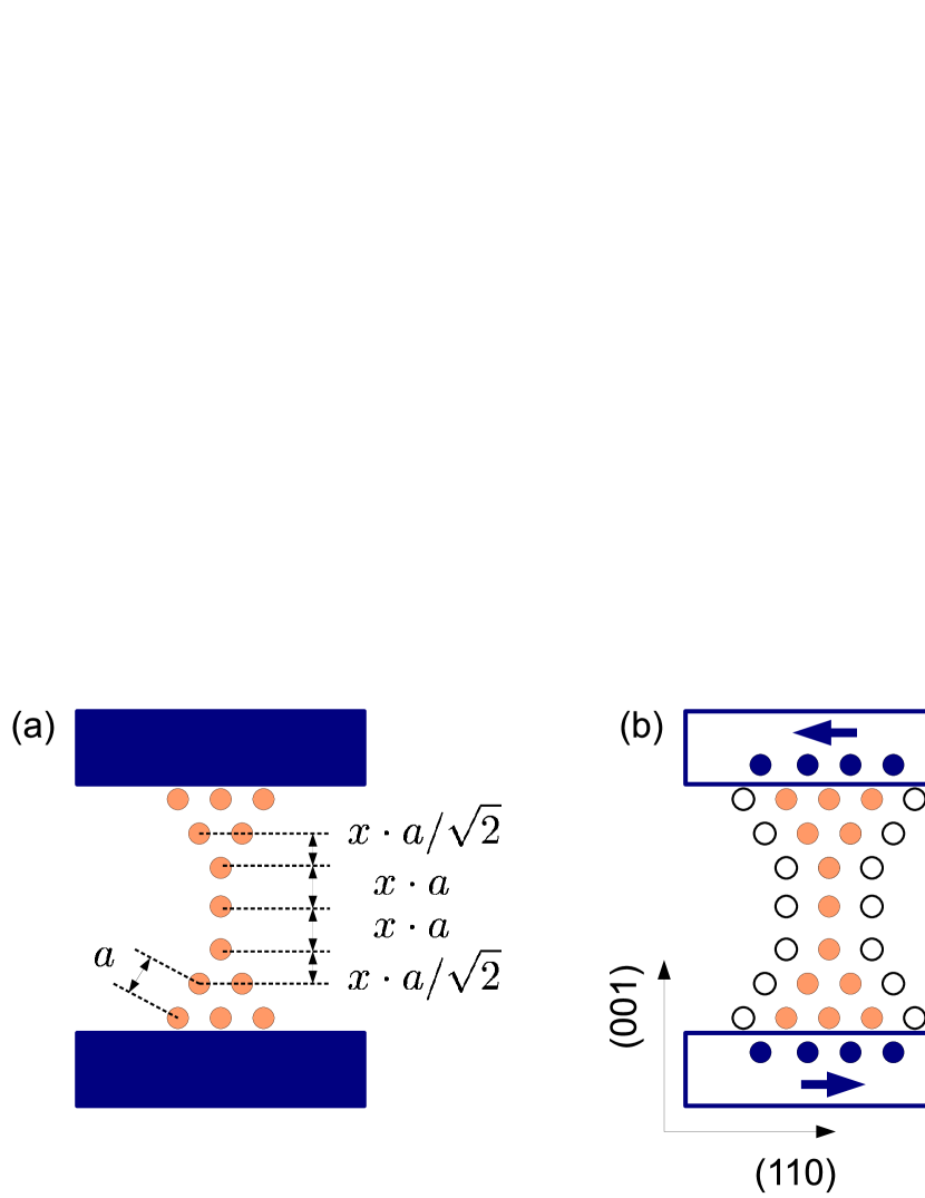
Figure 1: (Color online) (a) The geometry of the contact viewed from the $(1\overline{1}0)$ direction. The leads are depicted as dark (blue) rectangles, the cobalt atoms forming the contact are represented by gray (orange) circles, $a$ denotes the nearest neighbor distance in the fcc structure. The length of the contact is tuned via $x=$ 0.85, 0.90, 0.95, 1.00, 1.05, 1.10, and 1.15. Note that only the marked distances were scaled. (b) Sketch of the embedded cluster. Dark (blue) circles: selected atoms of the cobalt leads, gray (orange) circles: cobalt atoms in the nanocontact, and empty circles: empty spheres around the contact. The directions of magnetization in the leads are marked by dark (blue) arrows.

First, the electronic structure of the host was calculated in terms of the fully relativistic screened KKR method applying the surface Green’s function technique.Szunyogh et al. (1994a, b) Then the electronic structure of the contact has been determined within the EC-KKR method,Lazarovits et al. (2002) in which the scattering path operator (SPO), corresponding to a finite cluster, $\mathcal{C}$, embedded into a host system can be obtained from the following equation,

$$\bm{\tau}_{\mathcal{C}}(\varepsilon)=\left(\mathbf{t}_{\mathcal{C}}^{-1}(\varepsilon)-\mathbf{t}_{\text{h}}^{-1}(\varepsilon)+\bm{\tau}_{\text{h}}^{-1}(\varepsilon)\right)^{-1},$$ (1)

where $\mathbf{t}_{\text{h}}(\varepsilon)$ and $\bm{\tau}_{\text{h}}(\varepsilon)$ denote the single-site scattering matrix and the SPO matrix for the host confined to the sites in $\mathcal{C}$, respectively, while $\mathbf{t}_{\mathcal{C}}$ denotes the single-site scattering matrices of the embedded atoms. The calculations for both the host and the cluster were performed within the local spin-density approximation (LSDA),Vosko et al. (1980) by using the atomic sphere approximation (ASA) and $\ell_{\text{max}}=2$ for the angular momentum expansion.

A fully unconstrained extension of the relativistic EC-KKR method is used to find the magnetic configuration of the point contact. The evolution of the atomic magnetic moments is treated in a semi-classical manner similar to molecular dynamics, whereby, in spirit of the magnetic force theorem,Jansen (1999) the driving force is calculated as the derivative of the band energy,

$$E_{\text{b}}=\int\limits_{-\infty}^{\varepsilon_{\text{F}}}\left(\varepsilon-\varepsilon_{\text{F}}\right)n(\varepsilon)\,\mathrm{d}\varepsilon=-\int\limits_{-\infty}^{\varepsilon_{\text{F}}}N(\varepsilon)\,\mathrm{d}\varepsilon,$$ (2)

with respect to the transverse change of the exchange field, where $\varepsilon_{\text{F}}$ is the Fermi energy, while $n(\varepsilon)$ and $N(\varepsilon)$ stand for the density of states (DOS) and for the integrated DOS, respectively. In the multiple scattering formalism the exchange field enters the electronic structure via the single-site scattering matrix, $t_{i}$. The first and higher order changes of the $t_{i}$ matrices as well as the derivatives of the band energy can straightforwardly be calculated in the local frame of reference introduced at all sites of the cluster, where the direction vector $\bm{\sigma}_{i}$ of the magnetization at site $i$, and the two transverse vectors, $\mathbf{e}_{i1}$ and $\mathbf{e}_{i2}$, form a right handed coordinate system as shown in Fig. 2. The first and second order change of the single site scattering matrix at site $i$ with respect to rotations by $\Delta\phi_{i\alpha}$ around the transverse axes $\mathbf{e}_{i\alpha}$ can be given by the following commutator formulas,

$$\Delta t_{i}^{(1)} =i[\mathbf{e}_{i\alpha}\mathbf{J},t_{i}]\Delta\phi_{i\alpha},$$ (3)

$$\Delta t_{i}^{(2)} =-[\mathbf{e}_{i\alpha}\mathbf{J},[\mathbf{e}_{i\beta}\mathbf{J},t_{i}]]\Delta\phi_{i\alpha}\Delta\phi_{i\beta},$$ (4)

where $\mathbf{J}$ is the matrix representation of the total angular momentum operator and $\alpha,\beta\in\{1,2\}$. Following Ref. Udvardi et al., 2003, the first and second derivatives of the band energy can then be expressed as

$$\frac{\partial E_{\text{b}}}{\partial\phi_{i\alpha}} =\frac{1}{\pi}\,\mathrm{Re}\!\!\int\limits_{-\infty}^{\varepsilon_{\text{F}}}\!\!\mathrm{Tr}\left\{\tau_{ii}\left[\mathbf{e}_{i\alpha}\mathbf{J},m_{i}\right]\right\}\,\mathrm{d}\varepsilon,$$ (5)

$$\frac{\partial^{2}E_{\text{b}}}{\partial\phi_{i\alpha}\partial\phi_{j\beta}} =-\frac{1}{\pi}\mathrm{Im}\!\!\int\limits_{-\infty}^{\varepsilon_{\text{F}}}\!\!\mathrm{Tr}\left\{\tau_{ij}[\mathbf{e}_{j\beta}\mathbf{J},m_{j}]\tau_{ji}[\mathbf{e}_{i\alpha}\mathbf{J},m_{i}]\right\}\,\mathrm{d}\varepsilon$$

$$+\delta_{ij}\frac{1}{\pi}\mathrm{Im}\!\!\int\limits_{-\infty}^{\varepsilon_{\text{F}}}\!\!\mathrm{Tr}\left\{\tau_{ii}[\mathbf{e}_{i\alpha}\mathbf{J},[\mathbf{e}_{i\beta}\mathbf{J},m_{i}]]\right\}\,\mathrm{d}\varepsilon,$$ (6)

where $m_{i}=t_{i}^{-1}$ and $\tau_{ij}$ is the block of the SPO matrix between sites $i$ and $j$. Note that for brevity we dropped the energy arguments of the corresponding matrices in Eqs. (3–II). In the spirit of a gradient minimization, rotating the exchange field by a small amount around the torque vector at each sites,

$$\mathbf{T}_{i}=\mathbf{e}_{i1}\frac{\partial E_{\text{b}}}{\partial\phi_{i1}}+\mathbf{e}_{i2}\frac{\partial E_{\text{b}}}{\partial\phi_{i2}},$$ (7)

the magnetic configuration gets closer to the local minimum of the energy, however, the convergence is very slow. In order to speed up this procedure, a Newton-Raphson iteration scheme has been applied, where the inverse of the second derivative tensor, also referred to as the Hessian, Eq. (II), is used to estimate the angle of rotations around the torque vector given by Eq. (7). The eigenvalues of the Hessian also provide information about the stability of the a configuration with zero torque: if the Hessian is a positive or negative definite matrix then the given configuration is stable or unstable state of equilibrium, respectively. Once the Newton-Raphson iteration has converged, new effective potentials and exchange fields are generated and the procedure is repeated until the effective potential converged and the torque in Eq. (7) is decreased below a predefined value of, typically, $10^{-4}$ meV.

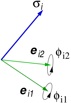
Figure 2: (Color online) Sketch of the local frame of reference: the unit vector $\bm{\sigma}_{i}$ is parallel to the magnetization at site $i$, while the unit vectors $\mathbf{e}_{i1}$ and $\mathbf{e}_{i2}$ point into the transverse directions. Rotations around these axes by $\phi_{i1}$ and $\phi_{i2}$ are also indicated.

The starting magnetic configuration for the above optimization procedure has been determined by Monte Carlo simulated annealing based on a simple isotropic Heisenberg model, $\mathcal{H}=\frac{1}{2}\sum_{i\neq j}J_{ij}\bm{\sigma}_{i}\bm{\sigma}_{j}$, where $J_{ij}$ is the isotropic exchange coupling between sites $i$ and $j$. The coupling coefficients between the atomic moments were calculated by using the torque method proposed by Liechtenstein et al. Liechtenstein et al. (1987) The exchange couplings have been calculated in a ferromagnetic spin-configuration parallel to the (100) direction.

In order to avoid the difficulties arising from the continuous degeneracy of the spin-states in a Heisenberg model, the magnetization on the central atom was fixed normal to the bulk magnetization. Considering the inversion symmetry of the point-contact, only the (1$\overline{1}$0) and the (001) directions are consistent with the (constrained) magnetic ground-state of the system. In the first case, the magnetic moments at all sites (layers) remain within the (001) plane, i.e., normal to the axis of the point-contact, therefore, in the following this spin-configuration will be termed as a helical domain wall. In the second case, all the spin moments are confined to the (1$\overline{1}$0) plane, thus, we shall call this case the cycloidal domain wall. Note that the helical and cycloidal spin-configurations closely resemble the Bloch and Néel types of domain walls well-known in bulk and thin-film magnets, respectively. Since, however, these types of domain walls are distinct through the magnetostatic energy, to avoid confusion we skipped using the traditional terminology.

III Results and discussions

III.1 Domain wall configurations

Self-consistent potentials and exchange fields have been first determined for both the cycloidal and the helical domain walls and the Newton-Raphson iterations were started from both initial configurations. Interestingly, when starting from a helical spin-configuration, the gradients, Eq. (5), were initially zero, but the Hessian had a negative eigenvalue indicating that the helical spin-configuration belonged to a saddle point of the energy surface. Throwing the system off this saddle point, the Newton-Raphson iterations converged to the cycloidal spin-configuration. Thus, independent of the starting configuration, the magnetic state of the nanojunction converged to the cycloidal wall structure for the stretching range considered. In Fig. 3 the ground-state cycloidal wall configuration is displayed for $x=1$.

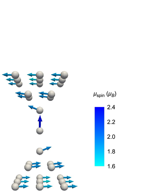
Figure 3: (Color online) The cycloidal spin-configuration obtained for the unstretched contact ($x=1$). The lengths of the arrows, indicated also with color coding, are proportional to the size of the spin magnetic moments.

At sites within the same geometrical layer, we obtained fairly similar orientations for the magnetic moments, therefore, the shape of the domain wall can well be characterized by orientations determined as an average within layers. In Fig. 4 such a profile is shown for $x=1$ in terms of polar angles, $\vartheta(z)$. Remarkably, the well-known analytical form, $\vartheta(z)=-\frac{\pi}{2}\tanh(2z/d_{\text{w}})$ could be well fitted defining, thus, the width of the domain wall, $d_{\text{w}}$. This fit is also shown in Fig. 4. We note that following Ref. Kazantseva et al., 2005 the analytical form of a constrained wall profile should be better described by Jacobian sine functions. However, testing this alternative approach resulted in to a relative deviation of less than 0.5 % in the fitted domain wall thicknesses.

Figure 4: Polar angles averaged within a layer of cobalt atoms in the contact with $x=1$ as the function of the distance from the central atom (in units of the fcc nearest neighbor distance, $a$). The solid curve displays the fit, $\vartheta(z)=-\frac{\pi}{2}\tanh(2z/d_{\text{w}})$.

Figure 5: Width of the domain walls through the point contact as a function of the stretching factor, $x$. Note that $d_{\text{w}}(1.00)=2.34\,a$, where $a$ is the fcc nearest neighbor distance. The solid line stands for the identity function.

The change of the width of the domain walls against the length of the point contact is shown in Fig. 5. For a clear interpretation, the width of the walls is normalized to the width of the domain wall for $x=1$. As obvious from this figure, $d_{\text{w}}(x)\approx x\,d_{\text{w}}(1.00)$ demonstrating that the width of the domain walls follows the length of the point contact. In case of Fe₂₀Ni₈₀ thin films it has been experimentally found that the constrained geometry can reduce the width of the Néel wall.Jubert et al. (2004) The effect is more pronounced in ultrathin films of few atomic layers where the width of the domain wall can be as small as few nanometers in the vicinity of a step edge.Pietzsch et al. (2000) The effect of the reduced dimensionality is even more obvious in the case of a point contact. Since the exchange energy gain for the few atoms of the contact is small compared to the increase of the exchange energy of the leads, the domain wall can not penetrate into the substrates and the wall is confined to the contact. The same conclusion has been drawn by BrunoBruno (1999) based on a theoretical study of a continuous model of domain walls in a confined geometry.

III.2 Magnetic moments

The low coordination in thin films and in nanostructures is often accompanied by the enhancement of the atomic spin and orbital moments. In Fig. 6 the calculated values of the local spin and orbital moments are given in a point contact with cycloidal wall configuration and stretching factor, $x=1$. Since the orbital moment is found almost parallel to the spin-moment at each site, we presented the projection of the orbital moment to the local spin quantization axis. Since the contact has a mirror symmetry with respect to the horizontal plane including the central atom, therefore, the moments in only one half of the contact are displayed. Our data fit nicely to the observation reported in Refs. Šipr et al., 2007 and Błoński and Hafner, 2009 that the spin and orbital moments at sites with lower coordination number are larger then at sites with larger coordination number. This is, in particular, true for the central atom with coordination number of only two where the values of the spin and orbital moments are even larger than those obtained for small clusters on Pt(111) and Au(111) surfaces.Šipr et al. (2007); Błoński and Hafner (2009); Lazarovits et al. (2003)

$\mu_{\text{spin}}\leavevmode\nobreak\ (\mu_{\text{B}})$
$\mu_{\text{orb}}\leavevmode\nobreak\ (\mu_{\text{B}})$

Figure 6: Calculated atomic magnetic moments ($\mu_{B}$) in half of the nanocontact for the stretching factor, $x=1$. In the upper and lower panels shown are the spin and orbital moments, $\mu_{\text{spin}}$ and $\mu_{\text{orb}}$, respectively. For comparison, the spin-moments at the Co surface and in the bulk are $1.82\,\mu_{\text{B}}$ and $1.67\,\mu_{\text{B}}/\text{atom}$, while the corresponding values of the orbital moments are $0.14\,\mu_{\text{B}}$ and $0.08\,\mu_{\text{B}}$.

Fig. 7 shows the spin and orbital moments of the central atom as a function of the stretching ratio $x$, for both the cycloidal and the helical spin-configurations in the point-contact. Clearly, the spin moments are fairly insensitive to the domain wall configuration: this can easily be understood as the relative spin-directions are nearly the same in the two types of domain walls. Also, there is only a moderate change of the spin moment in the range of $2.35\,\mu_{\text{B}}\leq\mu_{\text{spin}}\leq 2.49\,\mu_{\text{B}}$ for the stretching ratios under consideration. These values compare well to $\mu_{\text{spin}}=2.15\,\mu_{\text{B}}$ and $\mu_{\text{spin}}=2.26\,\mu_{\text{B}}$ calculated for a single Co adatom on Pt and Au(111) surfaces in Refs. Šipr et al., 2007 and Błoński and Hafner, 2009, respectively.

The dependence of the orbital moment of the central atom on the stretching is more pronounced than that of the spin moment: in case of a cycloidal and a helical wall it increases from about $1\,\mu_{B}$ to $2\,\mu_{B}$ and from $0.3\,\mu_{B}$ to $1.5\,\mu_{B}$, respectively. Similar high values of $\mu_{\text{orb}}$ for the central atom of a wire-like Fe point-contact were reported in Ref. Autès et al., 2008 and attributed to localized atomic-like electronic states treated within a full Hartree-Fock scheme. It should be mentioned that for a more reliable description of highly localized states, the plain LSDA we used in our calculations should be extended with, e.g., the local self-interaction correction, LSDA+SIC Lüders et al. (2005) or the dynamical mean field theory, LSDA+DMFT. Kotliar et al. (2006)

Apparently, the orbital moment of the central atom is systematically larger in a cycloidal wall than in a helical wall. This can be understood since these orbital moments correspond to different directions: in case of a cycloidal wall it points along the (001) directions, while, for a helical wall, along the (1$\overline{1}$0) direction. Such a huge anisotropy of the orbital moment at the central atom has also been observed in Ref. Autès et al., 2008. According to Bruno’s theory Bruno (1989) this large orbital momentum anisotropy is related to a large magnetic anisotropy energy featuring the (001) direction as easy axis, which clearly corroborates our result for the preference of a cycloidal domain wall.

Figure 7: The spin- and orbital moments of the central atom as a function of the stretching. Spin moments are displayed by open symbols, orbital moments are displayed by filled symbols as calculated in the cycloidal wall (CW, squares) and in the helical wall (HW, triangles) configurations.

III.3 Rotational energy of the domain wall

The cycloidal and helical spin-configurations of the point contact can be transformed into each other in term of a simultaneous rotation of the spin-directions around the axis parallel to the magnetization of the leads. The energy along the path of this global rotation, termed as the rotational energy of the domain wall, was calculated using the magnetic force theorem, namely, from the band energy of the system by rotating the orientation of the exchange field at each atomic site around the (110) axis and keeping frozen the effective potentials and fields as obtained for the ground state cycloidal wall configuration. For the case of the unstretched configuration the results are plotted in Fig. 8. The two minima and maxima of the band energy belong to the two-fold degenerate cycloidal and helical domain wall configurations. The height of the energy barrier between the two ground state cycloidal spin-configurations is 32.0 meV. Similar behavior has been found for the whole stretching range of the point contact. The energy differences between the two types of domain wall as a function of the stretching ratio are displayed by diamonds in Fig. 9.

Figure 8: The band energy of the nanocontact with $x=1.00$ while rotating the exchange field at each atomic sites simultaneously around the (110) axis. By rotating all the spins by $90^{\circ}$ the system goes over from the cycloidal wall (CW) into the helical wall (HW). The dashed line denotes the leading Fourier component of the band energy, $-15.2\;[\mathrm{meV}]\cos(2\theta)$, see Eq. (8). Note that we shifted the zero level of the energy to the constant term, $K_{0}$.

Due to time reversal symmetry, the magnetic anisotropy energy has a periodicity of $\pi$, but it does not comply with a usual $\cos^{2}(\theta)$ dependence. To explore this deviation we performed the Fourier expansion,

$$E_{\text{b}}(\theta)=K_{0}+\sum_{k=2,4,\dots}^{\infty}{K_{k}\cos(k\theta)}\,,$$ (8)

for the contacts with different stretching. Note that because of the inversion symmetry of the contact $E_{\text{b}}(\theta)=E_{\text{b}}(\pi-\theta)$ applies, therefore, the $\sin(k\theta)$ ($k=2,4,\dots)$ terms do not appear in the expansion, Eq. (8). We summarized the Fourier coefficients, $K_{k}$, in Table 1. We found that in each case the term $K_{2}\cos(2\theta)$ adds the largest weight to the rotational energy of the domain wall. The next term $K_{4}\cos(4\theta)$ is quite significant for $x\geq 0.95$, but it drops for smaller stretching. Interestingly, in the stretching range of $x\leq 0.90$ the $k=6$ term overweights the one of $k=4$, whereas in the complementary range the $k=6$ term is negligible. It should be mentioned that the $k\geq 8$ terms of the Fourier expansion have practically vanishing weight.

Table 1: The $k=2$, $4$ and $6$ Fourier coefficients (in units of meV) of the rotational energy of the point-contact, Eq. (8), as a function of the stretching parameter, $x$.

$x$	$k=2$	$k=4$	$k=6$
$0.85$	$-6.3$	$0.15$	$0.397$
$0.90$	$-10.0$	$0.36$	$0.499$
$0.95$	$-13.6$	$1.40$	$0.298$
$1.00$	$-15.2$	$2.17$	$-0.040$
$1.05$	$-15.1$	$2.35$	$-0.122$
$1.10$	$-14.4$	$2.24$	$-0.083$
$1.15$	$-13.2$	$1.92$	$0.025$

III.4 Magnetic anisotropy of the central atom

As we have seen in Sec. III.2, the central atom of the contact exhibits a huge orbital moment anisotropy that should be accompanied by a large magnetic anisotropy energy. For that reason, we analyze the band energy of the point-contact, $E_{\text{b}}(\bm{\sigma})$, with $\bm{\sigma}$ denoting the spin-orientation at the central atom, whereas the spin-orientations of all the other sites in the contact are kept fixed as obtained in the ground-state cycloidal wall configuration.

Our analysis is based on an expansion of $E_{\text{b}}(\bm{\sigma})$ in terms of (real) spherical harmonics, $R_{\ell}^{m}(\bm{\sigma})$,

$$E_{\text{b}}(\bm{\sigma})=\sum_{\ell,m}K_{\ell}^{m}R_{\ell}^{m}(\bm{\sigma})\,,$$ (9)

with the angular momentum indices, $\ell=0,1,2,\dots$ and $-\ell\leq m\leq\ell$. Similar to the rotational energy of the domain wall, we used the magnetic force theorem to evaluate $E_{\text{b}}(\bm{\sigma})$, but here we employed Lloyd’s formula, Lloyd (1967) since it accurately accounts for the change of the band energy of the whole point-contact with respect to the change of the spin-orientation at the central site. For the expansion, the integration over $\bm{\sigma}$ was performed using a 51 points Gaussian quadrature along the $z$-direction and a uniform mesh of 100 points in the azimuth angle, resulting in a spherical grid of 5100 points. The obtained coefficients are summarized in Table 2 up to $\ell=4$ and for all the stretching ratios under consideration. Only the non-vanishing coefficients are presented, for clarity, together with the definition of the corresponding spherical harmonics, $R_{\ell}^{m}(\bm{\sigma})$.

Table 2: Expansion coefficients $K_{\ell}^{m}$ (in units of meV) of the band energy of the contact, see Eq. (9), according to real spherical harmonics $R_{\ell}^{m}$ up to $\ell=4$.

$\ell$	$m$	$R_{\ell}^{m}\vphantom{\sqrt{\frac{1}{2}}}$	$x=0.85$	$x=0.90$	$x=0.95$	$x=1.00$	$x=1.05$	$x=1.10$	$x=1.15$
1	0	$\frac{1}{2}\sqrt{\frac{3}{\pi}}z$	$-240$	$-247$	$-235$	$-212$	$-192$	$-176$	$-159$
2	0	$\frac{1}{4}\sqrt{\frac{5}{\pi}}\left(3z^{2}-1\right)$	$-25.3$	$-30.0$	$-33.2$	$-32.4$	$-30.9$	$-28.4$	$-25.6$
2	2	$\frac{1}{4}\sqrt{\frac{15}{\pi}}\left(x^{2}-y^{2}\right)$	$4.30$	$2.54$	$1.39$	$0.51$	$-0.29$	$-0.92$	$-1.36$
3	0	$\frac{1}{4}\sqrt{\frac{7}{\pi}}\left(5z^{3}-3z\right)$	$4.12$	$3.06$	$1.63$	$0.71$	$-0.28$	$-1.43$	$-2.67$
3	2	$\frac{1}{4}\sqrt{\frac{105}{\pi}}\left(x^{2}-y^{2}\right)z$	$-0.199$	$-0.093$	$0.004$	$0.108$	$0.196$	$0.267$	$0.293$
4	0	$\frac{3}{16}\sqrt{\frac{1}{\pi}}\left(35z^{4}-30z^{2}+3\right)$	$-0.63$	$1.72$	$4.60$	$4.94$	$5.05$	$4.85$	$4.32$
4	2	$\frac{3}{8}\sqrt{\frac{5}{\pi}}\left(x^{2}-y^{2}\right)\left(7z^{2}-1\right)$	$0.033$	$0.125$	$0.184$	$0.108$	$0.051$	$0.001$	$-0.052$
4	4	$\frac{3}{16}\sqrt{\frac{35}{\pi}}\left(x^{4}-6x^{2}y^{2}+y^{4}\right)$	$-0.007$	$-0.005$	$-0.018$	$-0.041$	$-0.088$	$-0.187$	$-0.345$

The absence of certain spherical harmonics in expansion Eq. (9) can be discussed based on group-theoretical arguments. The function $E_{\text{b}}(\bm{\sigma})$ should be invariant under symmetry transformations, $g$, of the point-contact, $E_{\text{b}}(\bm{\sigma})=E_{\text{b}}(g\bm{\sigma})$, including the symmetry of both the lattice and the given (cycloidal) spin-configuration. Regarding that the spin-vectors transform as axial vectors, the only allowed transformation is the reflection onto the (001) plane: $(x,y,z)\rightarrow(-x,-y,z)$. Thus we conclude that only those function can enter the expansion of $E_{\text{b}}(\bm{\sigma})$ that contain even powers of the variables $x$ and $y$. As seen from Table 2, this is fully confirmed by our calculations. Apparently, the expansion Eq. (9) shows a satisfactory convergence as the coefficients rapidly decrease with increasing $\ell$. An obvious exception can, however, be seen for $K_{4}^{0}$ that for $x\geq 0.95$ overweights $K_{3}^{0}$. Noticeably, among the terms with a given $\ell$, the one associated with the $z$ component of the magnetization ($m=0$), i.e., excluding in-plane anisotropy, has the largest weight.

In order to connect the above results to the rotational energy of the domain wall discussed in Sec. III.3, we relate expansion Eq. (9) to a classical spin-model. According to a Heisenberg model extended by relativistic corrections Udvardi et al. (2003); Szunyogh et al. (2011) the energy in Eq. (9) can be expressed as

$$E(\bm{\sigma})=E_{\text{anis}}(\bm{\sigma})+\bm{\sigma}\sum_{j}\mathbf{J}_{\text{c}j}\bm{\sigma}_{j}\,,$$ (10)

where $\mathbf{J}_{\text{c}j}$ denote the exchange coupling tensor between the central site and the other sites of the contact with classical spin-vectors $\bm{\sigma}_{j}$ and $E_{\text{anis}}(\bm{\sigma})$ stands for the on-site anisotropy energy that, due to the tetragonal ($D_{4h}$) point-group symmetry of the point-contact, can be expanded up to $\ell=4$ as

$$E_{\text{anis}}(\bm{\sigma})=K_{2}^{0}R_{2}^{0}(\bm{\sigma})+K_{4}^{0}R_{4}^{0}(\bm{\sigma})+K_{4}^{4}R_{4}^{4}(\bm{\sigma})\,.$$ (11)

It is clear that the $(\ell,m)=(1,0)$ term in Eq. (9) is uniquely related to the exchange coupling and, due to the presence of a cycloidal wall, it represents a strong Weiss field that orients the magnetic moment at the central site along the $z$ direction. Because of the increasing distances between the central site and the other sites of the contact, it is also easy to understand why this term significantly decreases with increasing stretching ratio. On the other hand, there is no $(\ell,m)=(1,0)$ term in the rotational energy of the domain wall, Eq. (8), since in that case the relative orientation of the spins are unchanged. With other words, repeating the expansion Eq. (9) in the presence of a helical wall, the leading term correspond to the spherical harmonics $\propto x$, with practically the same coefficients as listed in Table 2 for $(\ell,m)=(1,0)$.

In relation to Eq. (11), the terms proportional to $R_{2}^{0}$, $R_{4}^{0}$ and $R_{4}^{4}$ in Eq. (9) can mainly be attributed to on-site anisotropy contributions to the spin-Hamiltonian, however, the effect of higher order spin-interactions can not be ruled out. The second-order uniaxial anisotropy coefficients, $K_{2}^{0}$, are negative in the whole range of stretching, favoring thus a normal-to-plane direction. Remarkably, the magnitude of $K_{2}^{0}$ is around 30 meV, with a maximum of $\left|K_{2}^{0}\right|=33.2\,\mathrm{meV}$ at $x=0.95$. This value should be compared to some results communicated in the literature: Etz et al. Etz et al. (2008) and Bornemann et al. Bornemann et al. (2007) calculated 5.3 meV and 4.76 meV, respectively, for the MAE of a Co ad-atom on Pt(111) surface, while, including orbital polarization, Gambardella et al. Gambardella et al. (2003) obtained 18.45 meV for the same system. In a similar geometrical confinement of an atomic scale junction, W and Ir turned out to be magnetic with a magnetic anisotropy energy comparable to our values.Thiess et al. (2010)

Figure 9: Diamonds: Calculated energy differences between the helical and cycloidal domain walls, $E_{\text{HW}}-E_{\text{CW}}$, circles: on-site uniaxial magnetic anisotropy energy of the central atom (see text) as a function of the stretching parameter, $x$. Thin lines serve as a guide for the eye.

From Fig. 8 and Table 1 we inferred that the rotational energy of the domain wall is dominated by the uniaxial magnetic anisotropy term proportional to $\cos^{2}\theta=z^{2}$. In Fig. 9 the energy differences obtained between the helical wall configuration and the ground state cycloidal wall configuration is plotted as a function of the stretching factor, together with that provided by the uniaxial anisotropy of the central atom, $\frac{3}{4}\sqrt{\frac{5}{\pi}}K_{2}^{0}$. The values of $\Delta E$ from the two calculations agree well for $x\geq 0.95$, while for more squeezed contacts the uniaxial anisotropy of the central atom overestimates the energy difference between the different types of domain walls. Nevertheless, we can in general conclude that the main driving force of the formation of a cycloidal domain wall is a giant uniaxial on-site magnetic anisotropy at the central atom: in the cycloidal wall the magnetic moment of the central atom is parallel to the easy axis, while in the helical wall configuration it lies within the hard plane.

Finally, we briefly comment on the terms corresponding to $(\ell,m)=(2,2)$, $(3,0)$, $(3,2)$ and $(4,2)$ in Table 2. Since these terms are not invariant under transformations of the $D_{4h}$ point-group, they can not be accounted for the on-site anisotropy terms. In terms of a spin-model, these terms should, therefore, be related to higher order spin-interactions. The $(\ell,m)=(2,2)$ term can, e.g., be identified as the consequence of biquadratic interactions,Deak et al. (2011) $\sum_{i}B_{\text{c}i}(\bm{\sigma}\bm{\sigma_{i}})^{2}$, while the $\ell=3$ terms to triquadratic interactions,Boča (2012) $\sum_{i}T_{\text{c}i}(\bm{\sigma}\bm{\sigma_{i}})^{3}$. Four-spin interactions have been explicitely calculated and proved to give significant contributions to a spin-Hamiltonian of Cr trimers deposited on Au(111) surface by Antal et al.,Antal et al. (2008) but recently their presence was highlighted even in bulk magnets. Lounis and Dederichs (2010)

IV Summary

In case of deposited magnetic nanostructures the point-group symmetry of the system might considerably be reduced, therefore, complex magnetic states occur naturally. Detecting and investigating such magnetic states pose a challenge for ab initio calculations. We have developed a computational technique based on a self-consistent embedded cluster Korringa-Kohn-Rostoker method suitable to find non-collinear ground-states of finite magnetic clusters. The method is applied to determine the structure of a domain wall formed through an atomic scale nanocontact between two antiparallelly magnetized cobalt leads. The obtained ground state is a cycloidal domain wall which remains stable against squeezing or stretching the contact along the normal-to-plane direction. A huge enhancement, as well as, anisotropy of the orbital moment are found at the central site of the contact. The energy of the domain walls was explored in terms of the magnetic force theorem. Our main observation is that the formation of the cycloidal wall against a helical wall is primarily driven by the uniaxial on-site anisotropy at the central site. We also found effects of higher order spin-interactions as terms in the expansion of the band energy not complying with the point-group symmetry of the point contact.