Geometric Phases generated by the non-trivial spatial topology
of static vector fields linearly coupled to a neutral spin-endowed particle.
Application to ¹⁷¹Yb atoms trapped in a 2D optical lattice

Abstract

We have constructed the geometric phases emerging from the non trivial topology of a space-dependent magnetic field ${\mathbf{B}}({\mathbf{r}})$, interacting with the spin magnetic moment of a neutral particle. Our basic tool, adapted from a previous work on Berry’s phases, is the space-dependent unitary transformation $\mathcal{U}({\mathbf{r}})$ which leads to the identity, $\mathcal{U}({\mathbf{r}})^{{\dagger}}\,{\mathbf{S}}\cdot{\mathbf{B}}({\mathbf{r}})\,\mathcal{U}({\mathbf{r}})=|{\mathbf{B}}({\mathbf{r}})|\,S_{z}$, at each point ${\mathbf{r}}$. In the “rotated” Hamiltonian $\widehat{\mathcal{H}}$, $\frac{\partial}{\partial{\mathbf{r}}}$ is replaced by the non-Abelian covariant derivative $\frac{\partial}{\partial{\mathbf{r}}}-\frac{i}{\hbar}\mathcal{A}({\mathbf{r}})$ where $\mathcal{A}({\mathbf{r}})=i\hbar\,\mathcal{U}^{{\dagger}}.\frac{\partial}{\partial{\mathbf{r}}}\mathcal{U}$ can be written as ${\mathbf{A}}_{1}({\mathbf{r}})S_{x}+{\mathbf{A}}_{2}({\mathbf{r}})S_{y}+{\mathbf{A}}_{3}({\mathbf{r}})S_{z}$. The Abelian differentials ${\mathbf{A}}_{k}({\mathbf{r}})\cdot d{\mathbf{r}}$ are given in terms of the Euler angles defining the orientation of ${\mathbf{B}}({\mathbf{r}})$. The non-Abelian field $\mathcal{A}({\mathbf{r}})$ transforms as a Yang-Mills field, however its vanishing “curvature” reveals its purely geometric character. We have defined a perturbation scheme based upon the assumption that in $\widehat{\mathcal{H}}$ the longitudinal field ${\mathbf{A}}_{3}({\mathbf{r}})$ dominates the transverse field ${\mathbf{A}}_{1,2}({\mathbf{r}})$ contributions, evaluated to second-order. The geometry embedded in both the vector field ${\mathbf{A}}_{3}({\mathbf{r}})$ and the geometric magnetic field $\mathbf{B}_{3}({\mathbf{r}})=\frac{\partial}{\partial{\mathbf{r}}}\wedge{{\mathbf{A}}}_{3}({\mathbf{r}})$ is described by their associated Aharonov-Bohm phase. As an illustration we study the physics of cold ¹⁷¹Yb atoms dressed by overlaying two circularly-polarized stationary waves with orthogonal directions, which form a 2D square optical lattice. The frequency is tuned midway between the two hyperfine levels of the $(6s6p)^{3}P_{1}$ states to protect the optical ${\mathbf{B}}({\mathbf{r}})$ field generated by the lattice from the dressed atom instability. The geometric field ${\mathbf{B}}_{3}({\mathbf{r}})$ is computed analytically in terms of the Euler angles. The magnitude of the second-order corrections due to the transverse fields can be reduced to the percent level by a choice of light intensity which keeps the dressed atom loss rate $\leq 5$ s^-1. A second optical lattice can be designed to confine the atoms inside 2D domains where ${\mathbf{B}}_{3}({\mathbf{r}})\cdot\hat{z}\geq 0$. We extend our analysis to the case of a triangular lattice.

I Introduction

In this paper we shall be interested in the spatial geometry associated with the time-independent Hamiltonian

$$\mathcal{H}=\frac{{\mathbf{p}}^{2}}{2\,M}+V({\mathbf{r}})-\gamma_{S}{\mathbf{S}}\cdot{\mathbf{B}}({\mathbf{r}}),$$ (1)

describing the quantum evolution of a non-relativistic neutral particle of spin S and magnetic moment $\gamma_{S}\;{\mathbf{S}}$, interacting with a scalar potential $V({\mathbf{r}})$ and a static non-uniform magnetic field ${\mathbf{B}}({\mathbf{r}})$.

In a recent work concerning Berry’s phases [8] generated by arbitrary spins non-linearly coupled to time-dependent external fields [9], we have found that the geometry of the Hamiltonian parameter space is more clearly exhibited if one uses a rotating frame method instead of the standard approach involving space-time wave functions within the adiabatic approximation. The Coriolis effect generates in the rotating frame a time-dependent linear spin coupling $\Delta H(t)=-\gamma_{S}\Delta{\mathbf{B}}(t).{\mathbf{S}}$. The Berry phase is generated by the longitudinal effective field $\Delta B_{z}(t)$ and the non-adiabatic corrections, governed by the transverse fields $\Delta B_{x,y}(t)$, are readily obtained by a second-order perturbation calculation.

The purpose of this paper is to use a similar approach to construct the geometrical phase associated with the non-trivial spatial topology of the magnetic field ${\mathbf{B}}({\mathbf{r}})$. We are going to apply to $\mathcal{H}$ a local unitary transformation, which makes diagonal the spin coupling at each point ${\mathbf{r}}$. The transformed kinetic term is obtained by replacing the gradient $\frac{\partial}{\partial{\mathbf{r}}}$ by the non-Abelian covariant derivative, ${\mathbf{D}}=\frac{\partial}{\partial{\mathbf{r}}}-\frac{i}{\hbar}{{\mathbf{A}}}_{k}({\mathbf{r}})S^{k}$ (with $S^{1}=S_{x},\;S^{2}=S_{y},\;S^{3}=S_{z}$), in which is encapsulated all the geometry of ${\mathbf{B}}({\mathbf{r}})$. By analogy with Berry’s phase it is possible to assume, within well-defined conditions, that the longitudinal field ${\mathbf{A}}_{3}({\mathbf{r}})$ gives the dominant contribution, the transverse ones, ${\mathbf{A}}_{1,2}({\mathbf{r}})$, leading to second-order corrections. This is a kind of Born-Oppenheimer approximation, playing, here, the role of the adiabatic approximation. The role of the Berry phase is, then, taken up by the Aharonov-Bohm phase associated with ${\mathbf{A}}_{3}({\mathbf{r}})$.

A simple example of this problem, where the spatial dependence of ${\mathbf{B}}({\mathbf{r}})$ results from a constant field gradient, was studied experimentally by W. Phillips and coworkers [1, 2]. In the case where ${\mathbf{B}}({\mathbf{r}})$ is a periodic field, $\mathcal{H}$ could be used, for instance as a model to describe the scattering of thermal neutrons by magnetic materials [3]. There has been recently a regain of interest in this model for describing the evolution of cold atoms within an optical lattice [4, 5, 6, 7]. ln this case, ${\mathbf{B}}({\mathbf{r}})$ stands for the “effective” magnetic field generated by an ac-Stark effect involving the electric field ${\mathbf{E}}({\mathbf{r}})$ associated with the coherent laser field used to construct the optical lattice. Two realistic and simple examples involving $S=1/2$ cold atoms trapped in a two-dimensional (2D) optical lattice will be discussed in the last section of this paper.

II Non-Abelian gauge fields generated by the ${\mathbf{B}}({\mathbf{r}})$ geometry

II.1 The “ rotated frame” approach

We are going to extend the method we have used in the case of time-dependent fields to the present context, by introducing at each space point ${\mathbf{r}}$ a “rotated frame”. The change of frame is defined by writing the vector state as $\Psi({\mathbf{r}})=\mathcal{U}({\mathbf{r}})\widehat{\Psi}({\mathbf{r}})$. The space-dependent unitary transformation $\mathcal{U}({\mathbf{r}})$ is designed to line up, at each space point, the magnetic field ${\mathbf{B}}({\mathbf{r}})$ along the spin quantization axis:

$$\mathcal{U}^{{\dagger}}({\mathbf{r}})\,{\mathbf{S}}\cdot{\mathbf{B}}({\mathbf{r}})\,\mathcal{U}({\mathbf{r}})=|{\mathbf{B}}({\mathbf{r}})|\,S_{z}.$$ (2)

Let us ignore, for a moment, that $\mathcal{U}({\mathbf{r}})$ does not commute with the kinetic energy term. For a periodic magnetic field, one would then have to solve, for each spin component $m$, a wave equation involving a scalar potential, like in the historical experiment of Stern and Gerlach. One would then come down to solving standard problems of solid state theory.

To proceed, let us introduce the rotation, ${\cal R}(\phi,\theta)=R(\hat{z},\phi({\mathbf{r}}))\cdot R(\hat{y},\theta({\mathbf{r}})),$ where $R(\hat{n},\chi)$ is the rotation of angle $\chi$ about the unit vector $\hat{n}$ and $\phi({\mathbf{r}}),\;\theta({\mathbf{r}})$ the two Euler angles which define the direction of the ${\mathbf{B}}({\mathbf{r}})$ field. More precisely, $\mathcal{R}(\phi({\mathbf{r}}),\theta({\mathbf{r}}))$ is chosen in order to satisfy the following equation,

$${\mathbf{B}}({\mathbf{r}})=|{\mathbf{B}}({\mathbf{r}})|\,\mathcal{R}(\phi({\mathbf{r}}),\theta({\mathbf{r}})).\hat{z}.$$ (3)

We should keep in mind that there is not a unique way to bring $\hat{z}$ along the direction of ${\mathbf{B}}({\mathbf{r}})$. This property can be associated with the gauge invariance of the non-Abelian gauge fields that we are going to introduce. It is easily verified that $\mathcal{U}({\mathbf{r}})$ given below coincides with the unitary transformation associated with the rotation $\mathcal{R}(\phi({\mathbf{r}}),\theta({\mathbf{r}}))$:

$$\mathcal{U}({\mathbf{r}})=\exp(\frac{-i}{\hbar}\,S_{z}\,\phi({\mathbf{r}})).\exp(\frac{-i}{\hbar}\,S_{y}\,\theta({\mathbf{r}})).$$ (4)

Using group theory arguments, one can derive the basic relation (see [9]),

$$\mathcal{U}^{{\dagger}}({\mathbf{r}})\,{\mathbf{S}}\,\mathcal{U}({\mathbf{r}})=\mathcal{R}(\phi({\mathbf{r}}),\theta({\mathbf{r}}))\cdot{\mathbf{S}}.$$ (5)

This leads to the set of identities: $\mathcal{U}^{{\dagger}}({\mathbf{r}})\,{\mathbf{S}}\cdot{\mathbf{B}}\,\mathcal{U}({\mathbf{r}})=(\mathcal{R}(\phi,\theta)\,{\mathbf{S}})\cdot{\mathbf{B}}={\mathbf{S}}\cdot(\mathcal{R}^{-1}(\phi,\theta)\,{\mathbf{B}})=|{\mathbf{B}}({\mathbf{r}})|\,S_{z}.$

II.2 The geometric non-Abelian gauge fields

Our next step is to write within the rotated frame the eigenvalue equation, $\mathcal{H}\,\Psi_{n}=E_{n}\Psi_{n}$, now taking into account that $\mathcal{U}({\mathbf{r}})$ does not commute with the kinetic energy operator $\frac{{\mathbf{p}}^{2}}{2\,M}$. By making simple manipulations, we arrive at the eigenvalue equation written in the rotated frame: $\widehat{\mathcal{H}}\,\widehat{\Psi}_{n}({\mathbf{r}})=E_{n}\widehat{\Psi}_{n}({\mathbf{r}})$, where the rotated Hamiltonian $\widehat{\mathcal{H}}=\mathcal{U}^{{\dagger}}({\mathbf{r}})\,{\mathcal{H}}\;\mathcal{U}({\mathbf{r}})$ is given by:

$$\widehat{\mathcal{H}} = \frac{1}{2\,M}\widehat{{\mathbf{p}}}^{2}+V({\mathbf{r}})-\gamma_{S}|{\mathbf{B}}({\mathbf{r}})|\,S_{z},$$ (6)

$$\widehat{{\mathbf{p}}} = -i\hbar\frac{\partial}{\partial{\mathbf{r}}}-i\hbar\,\mathcal{U}^{{\dagger}}({\mathbf{r}}).(\frac{\partial}{\partial{\mathbf{r}}}\mathcal{U}({\mathbf{r}})).$$ (7)

In reference ([9] sec. 4.2), we have made a similar calculation in the case where the Euler angles are time- instead of space-dependent. The needed result is obtained by doing the replacement: $\dot{\phi}\rightarrow\frac{\partial}{\partial{\mathbf{r}}}\,\phi\,,\,\dot{\theta}\rightarrow\frac{\partial}{\partial{\mathbf{r}}}\,\theta\,,\,\dot{\alpha}\rightarrow 0$. This leads to the following expression for $\widehat{{\mathbf{p}}}$:

$$\widehat{{\mathbf{p}}} = -i\hbar\frac{\partial}{\partial{\mathbf{r}}}-{{\mathbf{A}}}_{1}({\mathbf{r}})S_{x}-{{\mathbf{A}}}_{2}({\mathbf{r}})S_{y}-{{\mathbf{A}}}_{3}({\mathbf{r}})S_{z},$$

$${{\mathbf{A}}}_{1}({\mathbf{r}}) = -\sin\theta({\mathbf{r}})\,\frac{\partial}{\partial{\mathbf{r}}}\phi({\mathbf{r}}),$$

$${{\mathbf{A}}}_{2}({\mathbf{r}}) = \frac{\partial}{\partial{\mathbf{r}}}\theta({\mathbf{r}}),\;\;\;\;{{\mathbf{A}}}_{3}({\mathbf{r}})=\cos\theta({\mathbf{r}})\,\frac{\partial}{\partial{\mathbf{r}}}\phi({\mathbf{r}}).$$ (8)

Note that ${\mathbf{A}}_{3}({\mathbf{r}})\,S_{z}$, etc. are tensor products of a vector operator in the geometric space by a vector operator in the spin space. A remarkable feature of the above results is also the fact that the three fields ${{\mathbf{A}}}_{i}({\mathbf{r}})$ do not depend on the value of ${\mathbf{S}}^{2}=S(S+1)\hbar^{2}$. This follows from the fact that the evaluation of $\widehat{{\mathbf{p}}}$ relies only upon the $SU(2)$ Lie algebra: $[S^{i},S^{j}]=i\,\hbar\,{\epsilon}_{i\,j\,k}\,S^{k}$. A simple direct evaluation of the above formulas has been performed for $S=1/2$ using the fact that $\mathcal{U}({\mathbf{r}})$ is given by a $2\times 2$ matrix, linear with respect to ${\mathbf{S}}$. From now on, we shall often use the notation $S^{1}=S_{x},\;S^{2}=S_{y},\;S^{3}=S_{z}$ in order to stress that the $S^{i}$ will be treated as scalar objects under ordinary space rotation. It is of interest to incorporate the three fields ${{\mathbf{A}}}_{i}({\mathbf{r}})$ into a “non-Abelian” classical field $\mathcal{A}({\mathbf{r}})$, a well-known concept used in other fields of physics:

$$\mathcal{A}({\mathbf{r}})={{\mathbf{A}}}_{k}({\mathbf{r}})S^{k}=i\hbar\,\mathcal{U}^{{\dagger}}({\mathbf{r}}).(\frac{\partial}{\partial{\mathbf{r}}}\mathcal{U}({\mathbf{r}})).$$ (9)

The Hamiltonians considered in this work have not any simple invariance properties under rotation involving the total angular momentum of our neutral particle ${\mathbf{J}}={\mathbf{L}}+{\mathbf{S}}$. Using a fashionable expression, our spin will be treated as a “colored” spin.

II.3 Non-Abelian covariant derivatives and gauge invariance

In analogy with what is done for Abelian fields, we define the basic concept of covariant “derivative” as follows:

$${\mathbf{D}}=\frac{i}{\hbar}\widehat{{\mathbf{p}}}=\frac{\partial}{\partial{\mathbf{r}}}-\frac{i}{\hbar}{{\mathbf{A}}}_{k}({\mathbf{r}})S^{k}=\frac{\partial}{\partial{\mathbf{r}}}-\frac{i}{\hbar}\mathcal{A}({\mathbf{r}}).$$ (10)

We are now going to require that ${\mathbf{D}}.\widehat{\Psi}({\mathbf{r}})$ transforms under any space-dependent $SU(2)$ unitary transformation $\exp(\frac{i}{\hbar}\Lambda_{k}({\mathbf{r}})\,S^{k})$ in the same way as the wave function $\widehat{\Psi}({\mathbf{r}})$, i.e. $\widehat{\Psi}({\mathbf{r}})\rightarrow\widehat{\Psi}_{\Lambda}({\mathbf{r}})=\exp(\frac{i}{\hbar}\Lambda_{k}({\mathbf{r}})S^{k})\,\widehat{\Psi}({\mathbf{r}})).$ The above requirement will be satisfied provided that the non-Abelian field $\mathcal{A}({\mathbf{r}})$ is subjected to a well-defined non-Abelian gauge transformation: $\mathcal{A}({\mathbf{r}})\rightarrow\mathcal{A}_{\Lambda}({\mathbf{r}})$. The covariance condition means that the operator ${\mathbf{D}}$ should transform locally as a vector operator under any space-dependent $SU(2)$ unitary transformation:

$$\frac{\partial}{\partial{\mathbf{r}}}-\frac{i}{\hbar}\mathcal{A}_{\Lambda}=\exp(\frac{i}{\hbar}\Lambda_{k}S^{k})\,{\mathbf{D}}\,\exp(-\frac{i}{\hbar}\Lambda_{k}S^{k}).$$ (11)

The non-Abelian gauge transformation $\mathcal{A}({\mathbf{r}})\rightarrow\mathcal{A}_{\Lambda}({\mathbf{r}})$ is then easily derived by introducing in the above formula the expression of ${\mathbf{D}}$ given in Eq.(10),

$$\mathcal{A}_{\Lambda}({\mathbf{r}}) = \exp(\frac{i}{\hbar}\Lambda_{k}S^{k})\,\Big{(}\frac{i\,\hbar\partial}{\partial{\mathbf{r}}}\exp(-\frac{i}{\hbar}\Lambda_{k}S^{k})\Big{)}$$ (12)

$$+\exp(\frac{i}{\hbar}\Lambda_{k}S^{k})\,\mathcal{A}({\mathbf{r}})\,\exp(-\frac{i}{\hbar}\Lambda_{k}S^{k}).$$

It is found to agree with the formulas given by S. Weinberg [10] for general non-Abelian fields. If the space-dependent matrix $\Lambda_{k}({\mathbf{r}})S^{k}$ is replaced by an ordinary scalar function of ${\mathbf{r}}$, one recovers the usual Abelian gauge transformation.

An important physical concept for non-Abelian gauge fields is the “curvature” tensor, involving covariant derivative commutators, $\mathcal{F}_{i\,j}({\mathbf{r}})=i[D_{i},D_{j}]$, or

$$\mathcal{F}_{i\,j}({\mathbf{r}})=\frac{\partial}{\partial x_{i}}\mathcal{A}_{x_{j}}({\mathbf{r}})-\frac{\partial}{\partial x_{j}}\mathcal{A}_{x_{i}}({\mathbf{r}})-i[\mathcal{A}_{x_{i}},\mathcal{A}_{x_{j}}].$$

A crucial point, here, is that the non-Abelian field $\mathcal{A}({\mathbf{r}})$ given by equation (12) can be expressed under two forms, which are equivalent as a result of $\mathcal{U}({\mathbf{r}})$ unitarity: $\mathcal{A}({\mathbf{r}})=i\hbar\,\mathcal{U}^{{\dagger}}({\mathbf{r}})\,.\,(\frac{\partial}{\partial{\mathbf{r}}}\mathcal{U}({\mathbf{r}}))=-i\hbar(\frac{\partial}{\partial{\mathbf{r}}}\mathcal{U}^{{\dagger}}({\mathbf{r}}))\,.\,\mathcal{U}({\mathbf{r}}))$. Using this identity to rewrite $\mathcal{F}_{i\,j}({\mathbf{r}})$ one arrives, after some algebraic manipulations, at the remarkable result: $\mathcal{F}_{i\,j}({\mathbf{r}})=0$. This shows, clearly, that $\mathcal{A}({\mathbf{r}})$ is not a self interacting Yang-Mills field like the fields used in Particle Physics, but a purely geometrical field associated with a local change of space coordinates. There is a similarity with the situation encountered in the tests of the “equivalence principle” which involve “flat” space-time metrics.

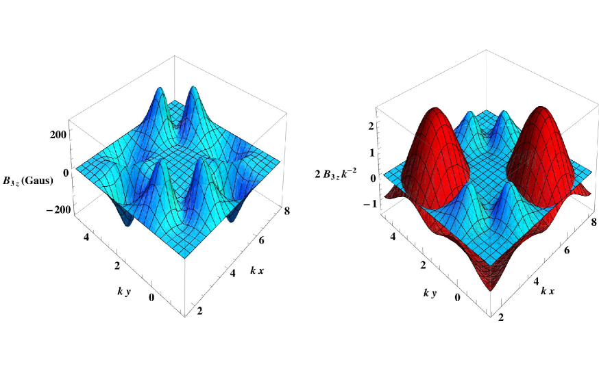
Figure 1: The geometric magnetic field $B_{3z}$ and the confinement potential inside one elementary cell of the optical lattice represented in the “rotated frame”. The Left graphic gives a perspective 3D plot of ${\mathbf{B}}_{em}({\mathbf{r}})$, the electromagnetic field equivalent of the geometric field ${\mathbf{B}}_{3}({\mathbf{r}})=\frac{\partial}{\partial{\mathbf{r}}}\wedge{{\mathbf{A}}}_{3}({\mathbf{r}})$, as a function of $k\,x$ and $k\,y$ ($k$ being the wave number of the optical “dressing” field generating the non-Abelian gauge fields). The geometric magnetic field $B_{3z}$ exhibits two positive maxima within the plaquette defined by $\pi/2\leq k\,x\leq 3\pi/2$, $-\pi/2\leq k\,y\leq\pi/2$. A symmetric pair of negative minima $B_{3z}$ appears within the plaquette obtained by performing the translation $x\rightarrow x+\pi$, as predicted by the formula (27). In the Right graphic we have plotted $B_{3z}$ together with the total potential $V_{c}({\mathbf{r}})=\mathcal{V}({\mathbf{r}})+\mathcal{W}({\mathbf{r}})-\gamma_{I}\,\hbar/2\,|{\mathbf{B}}({\mathbf{r}})|$ acting upon a state with $I_{z}=\hbar/2$, drawn in dark red using as unit $\gamma_{I}\,\hbar\,B_{0}$. ( For the sake of visibility $V_{c}({\mathbf{r}})$ has been shifted up by one unit.) As expected, the added potential $\mathcal{W}({\mathbf{r}})$ does prevent the cold atoms from exploring the regions where the sign of $B_{3z}$ is negative. Indeed, the pair of negative minima $B_{3z}$ of the Left are clearly not accessible for atoms below a well defined temperature. It is of interest to note that the two graphics are invariant under a rotation of $\pi$ around a vertical axis centered at the point $kx_{0}=3\pi/2,\,\,ky_{0}=\pi/2$, leading to the coordinate transformation, $x\rightarrow x^{\prime}=3\pi-x,y\rightarrow y^{\prime}=\pi-y$ which leaves invariant both $B_{3z}({\mathbf{r}})$ and $\mathcal{W}({\mathbf{r}}).$ The values of these quantities for the full 2D space are obtained by performing the set of translations: $x\rightarrow x^{\prime}=2\,n_{1}\,\pi+x,\,y\rightarrow y^{\prime}=2\,n_{2}\,\pi+y$ where $n_{1}$ and $n_{2}$ are arbitrary integers.

A possible application of the non-Abelian gauge transformation is the choice of the Landau gauge for ${{\mathbf{A}}}_{\Lambda 3}({\mathbf{r}})$ by writing ${A_{\Lambda 3x}=\hat{x}\cdot{\mathbf{A}}}_{\Lambda 3}({\mathbf{r}})=0$ without affecting the magnetic coupling. It is easily seen from Eq. (11), that the wanted gauge transformation has to satisfy the following constraints: $\widetilde{\Lambda_{1}}=\widetilde{\Lambda_{2}}=0\;,\;\frac{\partial}{\partial x}\,\widetilde{\Lambda_{3}}({\mathbf{r}})=-{A}_{3x}({\mathbf{r}}).$ An explicit expression $\widetilde{\Lambda_{3}}({\mathbf{r}})$ is obtained by a quadrature over $y:\widetilde{\Lambda_{3}}({\mathbf{r}})=-\int_{0}^{x}A_{3x}(v,y,z)\,dv.$ With this choice of $\Lambda$ the Hamiltonian $\widetilde{\mathcal{H}}$ is obtained from $\widehat{\mathcal{H}}$ by performing the replacement ${{\mathbf{A}}}_{i}({\mathbf{r}})\rightarrow{\widetilde{\mathbf{A}}}_{i}({\mathbf{r}})$,

$${\widetilde{\mathbf{A}}}_{1}({\mathbf{r}}) = \cos(\widetilde{\Lambda_{3}}){{\mathbf{A}}}_{1}({\mathbf{r}})+\sin(\widetilde{\Lambda{3}}){{\mathbf{A}}}_{2}({\mathbf{r}}),$$

$${\widetilde{\mathbf{A}}}_{2}({\mathbf{r}}) = -\sin(\widetilde{\Lambda_{3}}){{\mathbf{A}}}_{1}({\mathbf{r}})+\cos(\widetilde{\Lambda_{3}}){{\mathbf{A}}}_{2}({\mathbf{r}}),$$

$$\widetilde{{\mathbf{A}}}_{3}({\mathbf{r}}) = (A_{3y}({\mathbf{r}})+\frac{\partial}{\partial y}\widetilde{\Lambda_{3}}({\mathbf{r}}))\,\hat{y}.$$ (13)

III The Aharonov-Bohm phase from the “longitudinal” gauge field

Although the above developments are valid for any spin values, from now on, for sake of simplicity, we shall limit ourselves to the case of a $S=\frac{1}{2}$ particle in a 2D space. So far we have made no approximation. In analogy with the method we have used for Berry’s phases generated by non-linear spin Hamiltonians [9], we are going in sec. IV to construct a perturbation expansion, using as starting point the diagonal part ${\widehat{\mathcal{H}}}_{0}$ of the Hamiltonian $\widehat{\mathcal{H}}$,

$${\widehat{\mathcal{H}}}_{0} = -\frac{1}{2M}\big{(}\frac{\hbar\partial}{\partial{\mathbf{r}}}\big{)}^{2}+V({\mathbf{r}})+\frac{\hbar^{2}}{8\,M}\,\sum_{i=1}^{i=3}{\mathbf{A}}_{i}({\mathbf{r}})^{2}$$ (14)

$$-\big{(}\frac{i\hbar}{2\,M}\{\frac{\partial}{\partial{\mathbf{r}}},{{{\mathbf{A}}}}_{3}({\mathbf{r}})\}+\gamma_{S}|{\mathbf{B}}({\mathbf{r}})|\,\big{)}\,S_{z},$$

$\{...\}$ denoting the anticommutator between operators. The above approximation is often referred to as a Born-Oppenheimer (BO) approximation. It supposes that the evolution of the spin wave function is slow as compared to that of the spatial wave function describing the particle internal state (just like in molecular physics, the motion of the nuclei of a molecule is generally slow in comparison with that of the atomic electrons). The validity of this approximation in the present context is dicussed later on (see sec. IV). This is one advantage of the present “rotated” frame approach, similar to our treatment of the adiabatic approximation [9], to provide a systematic perturbation method to calculate the corrections. The left over perturbation Hamiltonian is given by the non-diagonal contribution of ${\widehat{\mathcal{H}}}$,

$${\widehat{\mathcal{H}}}_{1}=-\frac{i\hbar}{2\,M}\frac{\partial}{\partial{\mathbf{r}}}\cdot\big{(}{\mathbf{A}}_{1}({\mathbf{r}})S_{x}+{\mathbf{A}}_{2}({\mathbf{r}})S_{y}\big{)}+h.c.$$ (15)

Let us discuss the physics content of Eq. 14 for a given eigenvalue of $S_{z}/\hbar,\;m=\pm\frac{1}{2}$. The three first terms describe a spinless particle moving in a scalar potential. The terms of the second line represent the coupling of this particle of effective electric charge $m$, interacting with the Coulomb-like potential $-\gamma_{S}|{\mathbf{B}}({\mathbf{r}})|$ and a magnetic vector potential given by ${\mathbf{A}}_{3}({\mathbf{r}}).$ The diamagnetic term ${{\mathbf{A}}}_{3}({\mathbf{r}})^{2}$ is incorporated into the third term of the first line.

Ignoring for a moment ${\widehat{\mathcal{H}}}_{1}$, we would like to consider a two-slit Aharonov-Bohm interferometer experiment involving two beams described by wave packets, solutions of the Schrödinger equation associated with ${\widetilde{\mathcal{H}}}_{0}$. It is convenient to describe the two interfering beams by two Feynman path integrals associated with the classical paths $\mathcal{C}_{1}$ and $\mathcal{C}_{2}$ enclosing a 2D finite region $\mathcal{R}_{B}$ where the “geometric magnetic” field is confined:

$$\mathbf{B}_{3}({\mathbf{r}}) = \frac{\partial}{\partial{\mathbf{r}}}\wedge{{\mathbf{A}}}_{3}({\mathbf{r}})=\sin(\theta({\mathbf{r}}))\Big{(}\frac{\partial}{\partial x}\phi({\mathbf{r}})\,\frac{\partial}{\partial y}\theta({\mathbf{r}})-$$ (16)

$$\frac{\partial}{\partial y}\phi({\mathbf{r}})\,\frac{\partial}{\partial x}\theta({\mathbf{r}})\Big{)}\,\hat{z}.$$

Following Feynman [11], the phase difference

$$\Phi_{AB}(m)=-\,m\Big{(}\oint_{\mathcal{C}_{1}}\,{{\mathbf{A}}}_{3}({\mathbf{r}}_{1})\,d{{\mathbf{r}}}_{1}-\oint_{\mathcal{C}_{2}}\,{{\mathbf{A}}}_{3}({\mathbf{r}}_{2})\,d{{\mathbf{r}}}_{2}\Big{)},$$ (17)

is factored out of the functional integration and is given explicitly by the 2D integral:

$$\Phi_{AB}(m)=m\int_{\mathcal{R}_{B}}dx\,dy\,B_{3z}(x,y),$$ (18)

where $m\hbar$ plays the role of the electric charge. The Aharonov-Bohm phase [12] $\Phi_{AB}(m)$, can be viewed as a spatial extension of Berry’s phase associated with the non-trivial geometry of the physical ${\mathbf{B}}({\mathbf{r}})$ field, which is described by the geometric magnetic field, $\mathbf{B}_{3}({\mathbf{r}})$.

The above calculation has been performed in the rotated frame. To return to the laboratory frame, we shall use the fact that, in a typical Aharonov-Bohm experiment, the paths $\mathcal{C}_{1}$ and $\mathcal{C}_{2}$ are drawn in regions where $\mathbf{B}_{3}({\mathbf{r}})=0$. Assuming that the Feynman phase factors $\oint_{\mathcal{C}_{i}}\,{{\mathbf{A}}}_{3}({\mathbf{r}}_{i})\,d{{\mathbf{r}}}_{i}$ have been factored out, the wave functions relative to the paths $\mathcal{C}_{i}$ can be written in the rotated frame as $\widehat{\Psi}_{i,m}=\widehat{\psi}_{i,m}({\mathbf{r}},t)\otimes\widehat{\chi}_{m}$. The spatial wave functions $\widehat{\psi}_{i,m}({\mathbf{r}},t)$ obey the Shr$\ddot{o}$dinger equation associated with the Hamiltonian ${\widehat{\mathcal{H}}}_{0}({\mathbf{A}}_{3}=0,S_{z}=m\hbar)$ given by Eq. (14); $\chi_{m}$ is the $S=1/2$ spinor wave function, $(\delta_{m,1/2},\delta_{m,-1/2})$. When going back to the laboratory frame the spatial wave function $\widehat{\psi}_{i,m}({\mathbf{r}},t)$ is unchanged, whatever ${\mathbf{r}},t$, since $\mathcal{U}({\mathbf{r}},t)$ acts only on the spin, while the spinor, ${\chi}_{i,m}({\mathbf{r}})=\mathcal{U}({\mathbf{r}},t).\,\widehat{\chi}_{i,m}$ has been rotated. However, at the interference point the spinor wave function interference in the laboratory and in the rotated frame is identical, $\langle\widehat{\chi}_{2,m}|\widehat{\chi}_{1,m}\rangle=\langle\chi_{2,m}|\mathcal{U}^{\dagger}({\mathbf{r}}).\,\mathcal{U}({\mathbf{r}})|\chi_{1,m}\rangle$, as a consequence of the unitarity relation $\mathcal{U}^{\dagger}({\mathbf{r}}).\,\mathcal{U}({\mathbf{r}})=1$. In more physical terms the spins rotate differently along the two paths $\mathcal{C}_{1}$ and $\mathcal{C}_{2}$, but their scalar product is preserved at the interference point. In conclusion: $\Phi_{AB}^{lab}(m)=\Phi_{AB}(m)$.

In order to clarify the relation of $\Phi_{AB}(m)$ with the standard Berry’s phase, it is instructive to discuss briefly the case of a space and time-dependent ${\mathbf{B}}({\mathbf{r}},\,t)$ field. As before, let us construct the wave function in the frame rotating in space-time: $\widehat{\Psi}(t)=\mathcal{U}^{\dagger}({\mathbf{r}},t)\Psi(t)$, where $\Psi(t)$ is a solution of the Schrödinger equation associated with the time-dependent Hamiltonian $\mathcal{H}(t)$ obtained by giving a space- and time-dependence to the magnetic field ${\mathbf{B}}$. The unitary transformation $\mathcal{U}({\mathbf{r}},t)=\exp(\frac{-i}{\hbar}\,S_{z}\,\phi({\mathbf{r}},t)).\exp(\frac{-i}{\hbar}\,S_{y}\,\theta({\mathbf{r}},t))$ brings the ${\mathbf{B}}({\mathbf{r}},t)$ field along the $z$ axis. The time evolution of the “rotated” wave function is then governed by the Hamiltonian $\widehat{\mathcal{H}}(t)=\frac{1}{2M}(-i\hbar\frac{\partial}{\partial{\mathbf{r}}}-{{\mathbf{A}}}_{k}({\mathbf{r}},t)S^{k})^{2}-{V}_{k}({\mathbf{r}},t)S^{k}+V({\mathbf{r}})-\gamma_{S}|{\mathbf{B}}({\mathbf{r}},t)|\,S_{z}$. The scalar fields ${V}_{k}({\mathbf{r}},t)$ are obtained from the vector fields ${{\mathbf{A}}}_{k}({\mathbf{r}},t)$ by replacing in Eq. (8) $\frac{\partial}{\partial{\mathbf{r}}}$ by $\frac{\partial}{\partial t}$. For the moment, let us remove the ${\mathbf{r}}$ dependence and ignore the transverse potentials $V_{1,2}(t)$, governing the non-adiabatic corrections [9]. Berry’s phase is closely related to the dynamical phase contribution generated by $-V_{3}(t)S_{z}$ in the rotating frame [9]: $\widehat{\Phi}_{D3}=\int_{0}^{T}dt\,m\cos\theta(t)\,\dot{\phi}(t)$. By returning to the laboratory frame, $\widehat{\Psi}(t)\rightarrow\Psi(t)$, one recovers the standard Berry’s phase formula: $\beta(m)=\int_{0}^{T}dt\,m\big{(}\cos\theta(t)-1\big{)}\dot{\phi}(t).$

The creation of effective magnetic fields in 2D optical lattices was suggested by Jaksch and Zoller [13]. They deal with a pseudo spin $\frac{1}{2}$ associated with two internal atomic states. The effective fields are resulting from the spatial dependence of the Rabi frequencies induced by Raman lasers designed to transfer an atom in a given internal state to a nearest-neighbor lattice site associated with a flipped internal state. In addition, there is in the Hamiltonian a dynamical contribution which specifies the direction of the atomic jump. This requires, in practice, additional space-dependent potentials [14]. Here, we have adopted a totally different point of view: we have focused upon continuous space-dependent “dressed” Hamiltonians, having a linear spin coupling. We have developed a precise formalism showing how the non-trivial spatial topology of our spin Hamiltonian implies the existence of an Aharonov-Bohm phase, generated by a geometric magnetic field $\mathbf{B}_{3}({\mathbf{r}})$. The role of the electric charge is taken up by the eigenvalue of $S_{z}/\hbar,\,m=\pm\frac{1}{2}$.

IV The transverse gauge fields corrections

We are going to present a brief analysis of the effects or the transverse gauge fields ${{\mathbf{A}}}_{1,2}({\mathbf{r}})$ upon the physics associated with the approximation $\widehat{\mathcal{H}}\approx{\widehat{\mathcal{H}}}_{0}$, taking as an example the calculation of the Aharonov-Bohm phase. We shall use a perturbation approach using as starting point the eigenstates of ${\widehat{\mathcal{H}}}_{0}$ associated with a given eigenvalue of $m$: ${\widehat{\mathcal{H}}}_{0}\Psi_{n\,m}({\mathbf{r}})=E_{n\,m}\Psi_{n\,m}({\mathbf{r}})$. The eigenenergy corrections appear to be of second-order with respect to ${\widehat{\mathcal{H}}}_{1}$: $\Delta_{2}E_{n\,m}=\sum_{\bar{n}}|\langle\Psi_{n,m}|{\widehat{\mathcal{H}}}_{1}|\Psi_{\bar{n},-m}\rangle|^{2}\,/(E_{n,m}-E_{\bar{n},-m})$. Assuming that the magnetic coupling energy, $-\gamma_{S}S_{z}|{\mathbf{B}}({\mathbf{r}})|$, is dominant in ${\widehat{\mathcal{H}}}_{0}$ allows us to write: $E_{n,m}-E_{\bar{n},-m}$ as the quantum average of $-2m\,\gamma_{S}\,|{\mathbf{B}}({\mathbf{r}})|$. The energy shift $\Delta_{2}E_{n\,m}$ is then approximated by the rather simple expression:

$$\Delta_{2}E_{n\,m}\approx-\frac{\langle\Psi_{n,m}|{\widehat{\mathcal{H}}}_{1}^{2}|\Psi_{n,m}\rangle}{2\,m\,\hbar\gamma_{S}\,\langle\,\Psi_{n\,m}|\,(|{\mathbf{B}}({\mathbf{r}})|)\,|\Psi_{n\,m}\rangle}.$$ (19)

Let us now turn to the ${\widehat{\mathcal{H}}}_{1}$ corrections to the geometric phase $\Phi_{AB}(m)$. In a typical atomic interferometry experiment, the convergence of the two paths $\mathcal{C}_{i}$ is implemented with a localized “mirror” device. If the gauge vector field line integral is factored out, the wave packets $\Phi_{i}({\mathbf{r}},t)$ associated with $\mathcal{C}_{i}$ satisfy, outside the “reflexion” regions, the Schrödinger equation governed by ${\widehat{\mathcal{H}}}_{0}({{\mathbf{A}}}_{3}=0)$, a real operator having real eigenfunctions $\Phi_{n,m}$ with eigenvalues ${\cal E}_{n,m}$. Let us concentrate upon wave packets relative to the converging sections of the paths, $\Phi_{i}^{c}({\mathbf{r}},t)$ with $0<t<T$, where the times $-T,0,T$ are respectively the emission, reflexion and interference times. At these three times occur transformations described within the sudden approximation. Using standard time-dependent perturbation formalism, the first-order ${\widehat{\mathcal{H}}}_{1}$ corrections to the converging wave packets reads:

$$\delta\Phi_{i}^{c}(t) = 2\,i\sum_{n,\bar{n}}\langle\Phi_{\bar{n},-m}|{\widehat{\mathcal{H}}}_{1}|\Phi_{n,m}\rangle\langle\Phi_{n,m}|\Phi_{i}^{c}(0)\rangle$$

$$\times\;\frac{\sin(({\cal E}_{n,m}-{\cal E}_{\bar{n},-m})t/\hbar)}{({\cal E}_{n,m}-{\cal E}_{\bar{n},-m})}\,\,\Phi_{\bar{n},-m}.$$

Since only the wave packets with identical $m$ can interfere, the lowest-order interference correction reads: $\langle\;\delta\Psi_{2}^{c}(T)\,|\,\delta\Psi_{1}^{c}(T)\;\rangle=\langle\;\delta\Phi_{2}^{c}(T)\,|\,\delta\Phi_{1}^{c}(T)\;\rangle\,\exp(i\Delta\Phi_{AB}^{c})$, where $\Delta\Phi_{AB}^{c}$ is the phase difference accumulated along the converging paths. $\Delta\Phi_{AB}^{c}=m\big{(}\oint_{\mathcal{C}_{1}}\,{{\mathbf{A}}}_{3}({\mathbf{r}}_{1})\,d{{\mathbf{r}}}_{1}-(\mathcal{C}_{1}\rightarrow\mathcal{C}_{2})\big{)}.$ (Note the change of sign with respect to $\Phi_{AB}$.) To proceed we make two approximations. As before in the evaluation of $\Delta_{2}E_{n\,m}$ we shall write: $(\mathcal{E}_{n,m}-\mathcal{E}_{\bar{n},-m})={2\,m\,\gamma_{S}\,\langle\,\Psi_{n\,m}|\,(|{\mathbf{B}}({\mathbf{r}})|)\,|\Psi_{n\,m}\rangle}$. Then, we shall drop the oscillating $\sin$ products and replace the $\sin^{2}$ by their average $1/2$. This leads to the following expressions for $\delta_{1,2}^{c}=\langle\delta\Phi_{2}^{c}(T)|\delta\Phi_{1}^{c}(T)\rangle$ and $\eta_{n,m}$,

$$\delta_{1,2}^{c} \approx \sum_{n}\eta_{n,m}\;\langle\Phi_{2}^{c}(0)|\Phi_{n,m}\rangle\langle\Phi_{n,m}|\Phi_{1}^{c}(0)\rangle,$$

$$\eta_{n,m} = \frac{2\langle\Phi_{n,m}|{\widehat{\mathcal{H}}}_{1}^{2}|\Phi_{n,m}\rangle}{(\gamma_{S}\,\hbar\langle\,\Psi_{n\,m}|\,(|{\mathbf{B}}({\mathbf{r}})|)\,|\Psi_{n\,m}\rangle)^{2}},$$ (20)

which are closely related in magnitude to the energy shift $\Delta_{2}E_{n\,m}$, calculated previously (Eq. 19).

It is of interest to give an explicit expression of $\langle\Phi_{n,m}|{\widehat{\mathcal{H}}}_{1}^{2}|\Phi_{n,m}\rangle$, by writing ${\widehat{\mathcal{H}}}_{1}=\sum_{k=1}^{2}{\widehat{\mathcal{H}}}_{1,k}\,S^{k}$ where ${\widehat{\mathcal{H}}}_{1,k}=\{{\mathbf{p}}\ ,\,{\mathbf{A}}_{k}({\mathbf{r}})\}/(2\,M).$ Using the $S^{k}$ algebra for $S=1/2$, one gets the more compact expression,

$\langle\Phi_{n,m}|{\widehat{\mathcal{H}}}_{1}^{2}|\Phi_{n,m}\rangle=\sum_{k=1}^{2}\langle\Phi_{n,m}|{\widehat{\mathcal{H}}}_{1,k}^{2}|\Phi_{n,m}\rangle/4.$

Pulling out the ${\mathbf{A}}_{k}({\mathbf{r}})$ field from the matrix element of ${\widehat{\mathcal{H}}}_{1,k}$ one gets a formula useful for an explicit evaluation:

$$\langle\Phi_{n,m}|{\widehat{\mathcal{H}}}_{1}^{2}|\Phi_{n,m}\rangle = \frac{\hbar^{2}}{4\,M^{2}}\Big{\{}\sum_{k}\int d^{3}{\mathbf{r}}\,|\phi_{n,m}|^{2}(\frac{\partial}{2\,\partial{\mathbf{r}}}\cdot{\mathbf{A}}_{k})^{2}$$ (21)

$$+\sum_{k,i,j}\int d^{3}{\mathbf{r}}\frac{\partial}{\partial x_{i}}\Phi_{n,m}^{*}\,\frac{\partial}{\partial x_{j}}\Phi_{n,m}\times A_{k,i}\,A_{k,j}\Big{\}}$$

Using the above results which make no assumption about the origin of ${\mathbf{B}}({\mathbf{r}})$, it is possible to give an order of magnitude of $\eta_{n,m}$ in the particular case of a periodic field ${\mathbf{B}}({\mathbf{r}})$ associated with a single wave number ${\mathbf{k}}$. Looking at Eq. (8) one sees clearly that the non-abelian fields ${\mathbf{A}}_{i}({\mathbf{r}})$ scale as ${\mathbf{k}}$ and their divergence, $\frac{\partial}{\partial{\mathbf{r}}}\cdot{\mathbf{A}}_{i}({\mathbf{r}})$, as $k^{2}$. In an explicit computation to be presented later on, it appears that the terms involving the field divergence is the dominant one. Assuming that the magnetic coupling is the dominant term in ${\widehat{\mathcal{H}}}_{0}$, one arrives at the estimate,

$$|\eta_{n,m}|\lesssim\eta_{max}\;\;\;{\rm with}\;\;\eta_{max}=\frac{1}{2}\Big{(}\frac{(\hbar{\mathbf{k}})^{2}/(2\,M)}{\hbar\gamma_{S}{|{\mathbf{B}}({\mathbf{r}})|}_{min}}\Big{)}^{2},$$ (22)

which can also be viewed as a scaling law. In the case where the periodic field ${\mathbf{B}}({\mathbf{r}})$ contains an effective optical magnetic field ${\mathbf{B}}_{opt}({\mathbf{r}})$ generated inside a 2D optical lattice, $\ (\hbar{\mathbf{k}})^{2}/(2\,M)$ is the recoil energy of the cold atom following the absorption of one photon of momentum ${\mathbf{k}}$.

V Application to ${}^{171}\rm{Yb}$ cold atoms in a 2D optical lattice

We now want to illustrate the above theoretical analysis with a simple realistic example. We choose the case of cold neutral atoms with $F=I=\frac{1}{2}$ angular momentum, “dressed” by a second-order Stark effect [15] involving the wave electric field ${\mathbf{E}}({\mathbf{r}})$ of an optical lattice. The light wave directions and polarizations are selected to generate an effective magnetic field ${\mathbf{B}}_{opt}({\mathbf{r}})$ which has the lattice periodicity.

Much more ambitious experimental programs involving 2D optical lattices are aiming at a simulation of actual condensed matter problems [16, 17, 14, 18], like the electronic properties of graphene.

V.1 The dressed atom Hamiltonian $\mathcal{H}$

Let us assume that the “dressing” optical electric field ${\mathbf{E}}({\mathbf{r}})$ is obtained by the coherent superposition of two stationary waves, directed along $\hat{x}$ and $\hat{y}$. Each one results from the interference of a circularly polarized laser beam (wave vector ${\mathbf{k}}$, helicity $\xi$) and of the beam reflected at normal incidence, all beams carrying along their propagation axis the same angular momentum $\hbar\xi$ per photon,

$${\mathbf{E}}({\mathbf{r}}) = \mathcal{E}\Big{\{}\frac{1}{\sqrt{2}}(\hat{y}+i\xi\hat{z})(\exp{ik\,x}-\exp{-ik\,x})$$ (23)

$$+\frac{1}{\sqrt{2}}(\hat{z}+i\xi\hat{x})(\exp{ik\,y}-\exp{-ik\,y})\Big{\}}.$$

This configuration has been selected in order to make the space dependence of $i{\mathbf{E}}^{*}\wedge{\mathbf{E}}$ appearing in $\mathbf{B}({\mathbf{r}})$ both simple and symmetric under the $x\rightarrow y$ exchange (see Eq. (25) below). In particular the relative phase of the two stationary waves plays an essential role. To avoid the singularities of the non-Abelian gauge fields directly associated with the geometry of the optical “effective” magnetic field ${\mathbf{B}}_{opt}$, a uniform dc magnetic field ${\mathbf{B}}_{0}$ has to be applied, with the same $x\leftrightarrow y$ symmetry as ${\mathbf{B}}_{opt}$, ${\mathbf{B}}_{0}=(\sin{u}\;(\hat{x}+\hat{y})/\sqrt{2}+\cos{u}\;\hat{z})B_{0}$.

We consider non-interacting ¹⁷¹Yb atoms, with nuclear spin $\frac{1}{2}$, trapped in this 2D optical lattice and ignore many-body effects. The laser frequency is detuned from the transition at 555.8 nm between the ground state $(4f^{14},6s^{2})^{1}S_{0}$ and the first $(4f^{14},6s6p)^{3}P_{1}$ excited state. In the case of a single transition between two states of angular momentum $\frac{1}{2}$, the optical field generates a space-dependent effective dc magnetic field ${\mathbf{B}}_{opt}$ which follows from the identity, valid for $S=1/2$,

$$({\mathbf{S}}\cdot{\mathbf{E}}^{*})({\mathbf{S}}\cdot{\mathbf{E}})=\frac{\hbar^{2}}{4}{\mathbf{E}}^{*}\cdot{\mathbf{E}}+i\frac{\hbar}{2}{\mathbf{E}}^{*}\wedge{\mathbf{E}}\cdot{\mathbf{S}}.$$ (24)

The magnitude of ${\mathbf{B}}_{opt}$ scales as the atom-field coupling $\Omega^{2}/\delta$, where $\hbar\Omega=2\,\mathcal{E}\,d$ is the Rabi frequency of the transition, $d=\langle^{3}P_{0},\;m=0|d_{z}|^{1}S_{0}\rangle$ its electric dipole amplitude and $\delta$ the laser frequency detuning. Actually, the ¹⁷¹Yb isotope has two hyperfine (hf) components, $F=\frac{1}{2}$ and $F=\frac{3}{2}$ with relative strength $\frac{1}{3}$ and $\frac{2}{3}$ and hyperfine splitting $W_{hf}/\hbar=5.939$ GHz [19]. It is important to adjust the laser frequency midway between the two hf lines, (i.e. opposite detunings, $\hbar\delta=\pm W_{hf}/2$, for the two transitions). This particular choice has the great advantage of canceling out the imaginary part of the effective magnetic field associated with spontaneous emission (see Appendix). Only the number of dressed atoms, irrespective of their nuclear spin orientation, is subjected to a decrease. With this choice the contributions to ${\mathbf{B}}_{opt}$ coming from each transition happen to be equal.

It is convenient to write ${\mathbf{B}}_{opt}$ in a way which makes its coupling to the ¹⁷¹Yb ground state exactly similar to the real magnetic field coupling. Since it originates from an ac Stark shift, it has, however, no reason to have a vanishing divergence. From the calculation presented in the Appendix, Eqs. (35, 36), we obtain the expression,

$${\mathbf{B}}_{opt} = -\frac{8\,d^{2}}{3\,\gamma_{I}\,\hbar W_{hf}}\,i\,{\mathbf{E}}^{*}({\mathbf{r}})\wedge{\mathbf{E}}({\mathbf{r}})$$ (25)

$$=B_{0}\;\xi\,\rho\,\Big{(}\sin^{2}(k\,x)\hat{x}+x\rightarrow y-\sin(k\,x)\,\sin(k\,y)\hat{z}\Big{)},$$

$$\rho=\frac{32\,d^{2}\,\mathcal{E}^{2}}{3\,W_{hf}\,\hbar\,\gamma_{I}B_{0}}=\frac{8\;\hbar\Omega^{2}}{3\,W_{hf}\,\gamma_{I}B_{0}}.$$

Then, the dressed atom Hamiltonian is expressed as:

$$\mathcal{H} = \frac{{\mathbf{p}}^{2}}{2\,M}-\gamma_{I}({\mathbf{B}}_{0}+{\mathbf{B}}_{opt}({\mathbf{r}}))\cdot{\mathbf{I}}+\mathcal{V}({\mathbf{r}}),$$

$$\mathcal{V}({\mathbf{r}}) = -\;\hbar\gamma_{I}B_{0}\;\rho\;(\sin^{2}(k\,x)+\sin^{2}(k\,y))/4,$$ (26)

where the scalar potential $\mathcal{V}({\mathbf{r}})$ is associated with the scalar terms $\propto{\mathbf{E}}^{*}\cdot{\mathbf{E}}$ (see Eq. (35)).

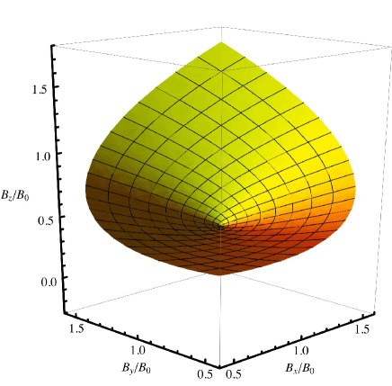
Figure 2: Illustration of the geometry embedded in the effective field ${\mathbf{B}}({\mathbf{r}})$ by a perspective view representing the 2D surface $\mathcal{S}$, immersed in a 3D Euclidian space. $\mathcal{S}$ is defined by the parametrization: $x_{1}=B_{x}(x,y)/B_{0}\,,y_{1}=B_{y}(x,y)/B_{0}\,,\,z_{1}=B_{z}(x,y)/B_{0}$. Performing the simple change of coordinates: $x_{2}=x_{1}-1/2=\sin^{2}(k\,x);y_{2}=y_{1}-1/2=\sin^{2}(k\,y);z_{2}=z_{1}-\sqrt{1/2}=-\sin(k\,x)\sin(k\,y)$, one finds that $\mathcal{S}$ is the intersection of a cone of equation: $z_{2}^{2}=x_{2}\,y_{2}$ with the cubic volume defined by $0<x_{2},~{}y_{2}<1$, together with the condition $-1<z_{2}<1.$ The “rotated” frame method is associated with the mapping of $\mathcal{S}$ onto a line segment along the $z_{1}$ axis. The cone tip can be associated with the saddle point appearing in Fig. 1 between two bumps of the geometric field $\mathbf{B}_{3}$.

V.2 Explicit evaluation of the phases associated with the magnetic field geometry

In the following, the AB phase will be considered as a diagnosis. It serves to test for the presence of a vector potential $\mathbf{A}_{3}({\mathbf{r}})$ able to generate the non-local quantum physical effects associated with the magnetic field ${\mathbf{B}}_{3}({\mathbf{r}})$.

We have all we need to construct the non-Abelian gauge fields given by Eqs. 8. The angles $\theta({\mathbf{r}})$ and $\phi({\mathbf{r}})$ appearing in the relevant unitary transformation: $\mathcal{U}({\mathbf{r}})=\exp(-\frac{i}{2}\sigma_{z}\,\phi({\mathbf{r}})).\exp(-\frac{i}{2}\,\sigma_{y}\,\theta({\mathbf{r}}))$ are given by the orientation of the total magnetic field, ${\mathbf{B}}({\mathbf{r}})={\mathbf{B}}_{0}({\mathbf{r}})+{\mathbf{B}}_{opt}({\mathbf{r}})$,

$$\tan\phi({\mathbf{r}}) = \frac{B_{y}({\mathbf{r}})}{B_{x}({\mathbf{r}})}\,,\,\;\;\;\;\cos\theta({\mathbf{r}})=\frac{B_{z}({\mathbf{r}})}{|B({\mathbf{r}})|}.$$

The graphs of Fig. 1 and 2 have been obtained for the typical case $u=\pi/4,\;\xi=\rho=1$. The geometric magnetic field $\mathbf{B}_{3}({\mathbf{r}})$ can, then, be obtained directly from the compact geometric formula (16). The algebraic structure of $\phi({\mathbf{r}})$ and $\theta({\mathbf{r}})$ suggests that $\mathbf{B}_{3}({\mathbf{r}})$ can be written under the symmetric form,

$$\mathbf{B}_{3}({\mathbf{r}}) = -\hat{z}\,k^{2}\cos(k\,x)\cos(k\,y)\,\mathcal{F}\big{(}\sin(kx),\sin(ky)\big{)},$$

$$\mathcal{F}(a,b) = (a^{2}+2\sqrt{2}a\,b+b^{2})G(a,b)^{-\frac{3}{2}},$$

$$G(a,b) = 1+a^{2}-\sqrt{2}a\,b+b^{2}+a^{4}+b^{4}+a^{2}\,b^{2}.$$ (27)

By looking at Fig.1, it is clearly of interest to compute the phase $\Phi_{geom}(1/2)$ as the flux of $m\,\mathbf{B}_{3}({\mathbf{r}})$ through the plaquette: $\pi/2\leq k\,x\leq 3\pi/2$, $-\pi/2\leq k\,y\leq\pi/2$. Using the above explicit expression of $\mathbf{B}_{3}({\mathbf{r}})$, and performing a precise numerical quadrature, one obtains $\Phi_{geom}(1/2)=0.499284$. This pure number is a characteristic of the geometry associated with ${\mathbf{B}}({\mathbf{r}})$ for the values of the geometric parameters $u=\pi/4,\;\xi=\rho=1$.

It is of interest to construct, from the geometric field ${\mathbf{B}}_{3}({\mathbf{r}})$, an electromagnetic field which would induce the same physical effect (e.g. the same Aharonov-Bohm phase for a particle with elementary electric charge $e$). This can be achieved by comparing the covariant derivative of Eq.(10), in the limit ${{\mathbf{A}}}_{1}({\mathbf{r}})={{\mathbf{A}}}_{2}({\mathbf{r}})=0$ (namely $\frac{\partial}{\partial{\mathbf{r}}}-i\,m\,{{\mathbf{A}}_{3}}({\mathbf{r}})$, $m\hbar$ being the eigenvalue $\pm\frac{1}{2}$ of $I_{z}$), with the corresponding expression in the electromagnetic case: $\frac{\partial}{\partial{\mathbf{r}}}-i\frac{e}{\hbar}\,{\mathbf{A}}_{em}({\mathbf{r}})$. A simple inspection leads to: ${\mathbf{A}}_{em}({\mathbf{r}})=m\frac{\,\hbar}{e}{{\mathbf{A}}_{3}}({\mathbf{r}})$. This implies ${\mathbf{B}}_{em}({\mathbf{r}})=\pm\frac{1}{2}(\frac{2\pi}{\lambda({\rm Yb})})^{2}\frac{\,\hbar}{e}(\mathbf{B}_{3}({\mathbf{r}})k^{-2})$, where $\lambda({\rm Yb})=0.5558\times 10^{-6}m$ is the wavelength of the ${}^{1}S_{0}\rightarrow\,^{3}P_{1}\,^{171}$Yb transition. Using the values of $e$ and $\hbar$, one gets the electromagnetic equivalent in $MKSA$ units of the geometric field ${\mathbf{B}}_{3}({\mathbf{r}})$, ${\mathbf{B}}_{em}({\mathbf{r}})=\pm 0.0420287\times 10^{4}$ T$\times(\mathbf{B}_{3}({\mathbf{r}})\,k^{-2}$).

It is important to note that in the expression of $B_{3z}$, Eq. (27), $\mathcal{F}(\sin(kx)\sin(ky))$ is a positive definite function of $x,y$. This suggests the possibility to confine the Yb atoms in 2D domains where $\mathbf{B}_{3}({\mathbf{r}})\cdot\hat{z}\geq 0$, by adding to the $\mathcal{H}$ Hamiltonian an extra scalar potential,

$$\mathcal{W}({\mathbf{r}})=\hbar\gamma_{I}\;B_{0}\,\mu\,\cos(k\,x)\cos(k\,y),$$ (28)

where $\mu$ is a dimensionless positive parameter to be adjusted. Let us write, in the “rotated” frame, the confining part of the ${\widehat{\mathcal{H}}}_{0}$ Hamiltonian associated with the dressed $(4f^{14}~{}6s^{2})^{1}S_{0},\;I=\frac{1}{2}$ ground state of ¹⁷¹Yb,

$${\widehat{\mathcal{H}}}_{c}=\frac{{\mathbf{p}}^{2}}{2\,M}+\Big{(}\mathcal{V}({\mathbf{r}})+\mathcal{W}({\mathbf{r}})-\gamma_{I}\;|{\mathbf{B}}({\mathbf{r}})|\,I_{z}\Big{)}.$$ (29)

We have omitted the gauge vector fields $\mathbf{A}_{i}({\mathbf{r}})$ contributions, which play a limited role in the confinement. In the rhs of Fig. 1, we have plotted in red, using $\gamma_{I}B\hbar$ units, the total potential acting on the hyperfine sub-state $I_{z}=\hbar/2$,

$$V_{c}({\mathbf{r}})=\mathcal{V}({\mathbf{r}})+\mathcal{W}({\mathbf{r}})-\gamma_{I}\,\hbar/2\,|{\mathbf{B}}({\mathbf{r}})|.$$ (30)

We have found that the choice $\mu=2$ leads to the wanted effect. On the same graph, we have displayed in blue twice the dimensionless quantity $\mathbf{B}_{3}({\mathbf{r}})\,k^{-2}$. It is clear that, for an appropriate temperature, cold ¹⁷¹Yb atoms can be confined in connected domains of the 2D-space where the effective magnetic field satisfies $\mathbf{B}_{3}({\mathbf{r}})\cdot\hat{z}\geq 0$. For this purpose, the experiment should make use of two optical lattices having the same periodicity, but each one fulfilling a different role. The green lattice (555.8 nm) provides the topology of the effective field which generates the geometric non-Abelian field and the associated AB phase. The confinement role is attributed to the second lattice, spin-decoupled, hence not affected by the “rotated” frame transformation. This provides the possibility to adjust the atom position according to their temperature.

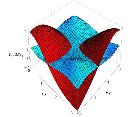
Figure 3: The scalar potential $V_{c}({\mathbf{r}})$ (dark red) and the geometric field $B_{3z}$ (light blue), within one quarter of the elementary cell relative to the potential $\mathcal{W}({\mathbf{r}})$. The geometric phase relative to this plaquette cancels, but when $\mathcal{W}({\mathbf{r}})$ is increased adiabatically, the trajectory of the wave packet is clearly modified: the cold atom is attracted towards the $B_{3z}>0$ regions and gets submitted to a Laplace-type force. The quantum circuit no longer satisfies the conditions required for the observation the AB effect. Therefore the cancellation of the purely geometric phase no longer implies the vanishing of the magnetic flux through a physical circuit, hence cannot be considered as a negative test of the $B_{3z}$ field relevance.

One way to generate the scalar potential $\mathcal{W}({\mathbf{r}})$ is to rely upon the scalar ac Stark effect with a large detuning. This may involve two stationary waves linearly polarized along $\hat{z}$, having wave vectors ${{\mathbf{k}}}_{1}=k(\hat{x}+\hat{y})/2$ and ${{\mathbf{k}}}_{2}=k(\hat{x}-\hat{y})/2$ with $|{{\mathbf{k}}}_{1}|=|{{\mathbf{k}}}_{2}|=k/\sqrt{2}$, i.e. $\lambda=786.0$ nm. We make the further assumption that there is no phase coherence between the two stationary waves, in other words, they do not interfere. With an appropriate phase and intensity matching of each stationary wave, the light induced potential, up to a constant factor, is given by: $\cos(\ k\,(x+y)/2)+\cos(\ k\,(x-y)/2)=2\,\cos(k\,x)\cos(k\,y)$. It has clearly the right space dependence for the wanted potential and the wanted sign is provided by the negative red detuning. The light intensity can be used to adjust the potential depth without affecting the stability of the dressed atoms, thanks to the large magnitude of the detuning $\simeq 10^{8}\,\Gamma_{P}$.

An important property of the flux of ${\mathbf{B}}_{3}$ is its cancellation when it is taken through a full elementary cell. This is an obvious consequence of the periodicity of the gauge vector field ${\mathbf{A}}_{3}({\mathbf{r}})$ generated by the periodic optical field ${\mathbf{B}}_{opt}({\mathbf{r}})$. From a look at Fig.1, it is clear that the symmetry properties of $\mathbf{{\mathbf{B}}}_{3}$ imply that its flux $\Phi_{geom}$ through the plaquette now associated with the half-elementary cell, defined by $\pi/2\leq kx\leq 5\pi/2\,,\,-\pi/2\leq ky\leq\pi/2$, vanishes. The vanishing of $\Phi_{geom}$ - a purely geometrical result - is not affected by the scalar potential $\mathcal{W}({\mathbf{r}})$ which has no effect upon the ${{\mathbf{A}}}_{3}({\mathbf{r}})$ gauge field. In the limit where the kinetic term dominates $V_{c}({\mathbf{r}})$ in the Hamiltonian ${\widehat{\mathcal{H}}}_{c}$, it is possible to build wave packets which propagate along the plaquette perimeter. The AB phase, $\Phi_{AB}$, around the half-elementary cell will vanish since it coincides with $\Phi_{geom}$. However, if we assume that $\mathcal{W}({\mathbf{r}})$ is increased adiabatically, the wave packets are pushed towards the regions where $B_{3z}>0$. Depending on their kinetic energy, they may even be confined there. In these conditions, the phase accumulated along the deformed circuit will differ from $\Phi_{geom}$ for two reasons: first, the $B_{3z}$ flux is no longer guaranteed to vanish; second, the wave packets propagate in regions where $|B_{3z}|>0$ which makes the situation incompatible with physical requirements for measuring the AB effect, see Fig. 3. Therefore the vanishing of the $B_{3z}$ flux through this particular purely geometric loop cannot be considered as an evidence for the irrelevance of the ${\mathbf{B}}_{3}$ field in presence of a confining potential.

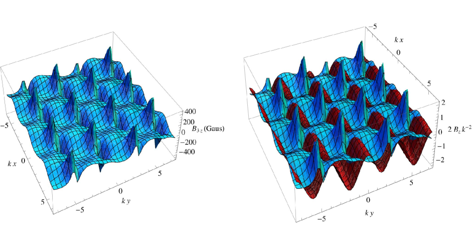
Figure 4: The geometric field ${\mathbf{B}}_{3}({\mathbf{r}})$ (in light blue) and the scalar confinement potential (in dark red) for the triangular optical lattice within the rotated frame. Left : The holes and the bumps of ${\mathbf{B}}_{3}({\mathbf{r}})$ form an hexagonal lattice. They can be organized in rows alined along the $x$-axis. Right : This can be used to introduce in $\widehat{\mathcal{H}}$ an extra $y$-dependent $\mathcal{W}({\mathbf{r}})$ potential leading to the total scalar potential $V_{c}({\mathbf{r}})$ acting on the state $I_{z}=\hbar/2$ (in $\gamma_{I}\hbar\,B^{tri}_{0}$ units). For sake of visibility $V_{c}({\mathbf{r}})$ is shifted up by 1 unit.

V.3 The instability of the dressed atom versus the transverse field corrections

By contrast to what happens for ${\mathbf{B}}_{opt}$, the imaginary part of the scalar potential $\mathcal{V}({\mathbf{r}})$ does not cancel out. This leads to an instability of the “dressed” atom associated with the spontaneous decay of the mixed excited state [20, 15]. However, the long lifetime $\Gamma_{P}^{-1}=850$ ns of the ${}^{3}P_{1}$ atomic state [21] contributes to slow down the decay of the dressed atom governed by the rate $\Gamma^{\prime}=(4\hbar^{2}\Omega^{2}/W_{hf}^{2})\Gamma_{P}$ for the chosen detuning (see Appendix). There is a clear relation between the magnitudes of $B_{opt}$ and $\Gamma^{\prime}$ since they are both proportional to $\Omega^{2}$, hence to the laser intensity $I_{l}$. Following the current use, the laser intensity is defined in terms of the saturated intensity $I_{s}$ at which $\Omega^{2}=\Gamma^{2}/2$. For the Yb transition considered, $I_{s}$ amounts to 0.14 mW/cm² [22] leading to a decay rate $\Gamma^{\prime}=1$ s^-1, obtained for a laser intensity $I_{l}$= 73 mW/cm² which gives rise to $B_{opt}=4.824$ G. Obviously, the laser intensity will have to satisfy a compromise if one wants to keep $\Gamma^{\prime}\propto I_{l}$ small as well as the parameter $\eta\propto I_{l}^{-2}$ which scales the importance of the transverse gauge field corrections. Below we show that a realistic compromise does exist, allowing one to anticipate a magnitude of corrections at the percent level.

To get a more precise evaluation of the transverse gauge field corrections than the one given in equation (22), we have calculated numerically the average of the two quantities $\mathcal{N}=\sum_{i=1,2}(\frac{\partial}{\partial{\mathbf{r}}}\cdot{\mathbf{A}}_{i}({\mathbf{r}}))^{2}$ and $|B({\mathbf{r}})|$, using their exact expressions over the relevant plaquette. In the rhs of Eq. (21), the second term, once averaged, is found to be ten times smaller than the first one, whose average leads to $\mathcal{N}_{av}=1.53445~{}k^{4}$, while ${|B({\mathbf{r}})|}_{av}=1.684~{}B_{0}$. From their ratio and the value of $\eta_{0}=\frac{1}{2}\Big{(}\frac{(\hbar{\mathbf{k}})^{2}/(2\,M)}{\hbar\gamma_{S}B_{0}}\Big{)}^{2}=12.64$ for ¹⁷¹Yb and for $B_{0}=1$ gauss. We deduce $\eta_{av}=\eta_{0}\,\mathcal{N}_{av}/{|B({\mathbf{r}})|}_{av}=6.828~{}B_{0}^{-2}$ (for $B_{0}$ expressed in gauss). This gives an improved estimate of $\eta_{n,m}$ (Eq. (22)) in this well specified geometry, assuming that the Bloch wave functions moduli are slowly varying over one elementary cell. One can reduce $\eta_{av}$ to the one percent level, by choosing $B_{0}=24$ G. For the total laser intensity this leads to $I_{l}=365$ mW/cm², shared among the four beams, with ${\Gamma^{\prime}}^{-1}=0.2$ s for the “dressed” ground state lifetime.

V.4 Extension to a triangular optical lattice involving running waves

To end this section, we would like to present an extension of the above analysis to the case a triangular optical lattice, generated by a set of three interfering running waves, invariant by rotation of $2\pi/3$-multiple angles. The triangular geometry has been observed for the first time by Grynberg et al. [23] and the properties of cold atoms trapped in such a 2D lattice have already been considered in [24] but with a spatial configuration different from the one adopted here. In contradistinction to what we do, the authors have not taken into account the two hyperfine transitions.

We consider three circularly polarized, running waves, which propagate in the $x,\,y$ plane. It should be noted that the previous square lattice built from stationary waves cannot be identified with a running wave lattice invariant by rotation of $\pi/2$-multiple angles, since the normal reflexion of an optical wave cannot be described by a rotation of $\pi$ of the wave electric field. Our optical triangular lattice is described by the following optical electric field,

$${\mathbf{E}}({\mathbf{r}}) = \mathcal{E}\sum_{n=0}^{n=2}\,{\mathbf{e}}_{n}(\xi)\exp(i{\mathbf{k}}_{n}-i\zeta(n)),$$

$${\mathbf{k}}_{n} = R(\hat{z},2n\pi/3).\hat{x},$$

$${\mathbf{e}}_{n}(\xi) = R(\hat{z},2n\pi/3).(\hat{y}+i\xi\hat{z})/\sqrt{2}.$$ (31)

It turns out that the choice $\zeta(n)=2n\pi/3$ is slightly more favorable than $\zeta(n)=0$. To simplify the writing, it is convenient to introduce the dimensionless vector field: ${\mathbf{b}}({\mathbf{r}})=-\frac{i}{2\,\mathcal{E}^{2}}{\mathbf{E}}^{*}({\mathbf{r}})\wedge{\mathbf{E}}({\mathbf{r}})$. Performing a straightforward computation using the above expression of ${\mathbf{E}}({\mathbf{r}})$, one arrives at the rather compact expressions for the ${\mathbf{b}}({\mathbf{r}})$ field components:

$$b_{x}=\frac{\xi}{2}\Big{(}-\cos\big{(}\sqrt{3}y-2\zeta\big{)}+\cos\big{(}\frac{3x}{2}\big{)}\cos\big{(}\frac{\sqrt{3}y}{2}-\zeta\big{)}\Big{)},$$

$$b_{y}=\frac{\xi}{2}\sqrt{3}\sin\big{(}\frac{3x}{2}\big{)}\sin\big{(}\frac{\sqrt{3}y}{2}-\zeta\big{)},$$

$$b_{z}=\frac{\sqrt{3}}{2}\sin\big{(}\frac{\sqrt{3}y}{2}-\zeta\big{)}\Big{(}\cos\big{(}\frac{3x}{2}\big{)}-\cos\big{(}\frac{\sqrt{3}y}{2}-\zeta\big{)}\Big{)}.$$

By contrast to the previous case, $b_{z}$ is independent of the beam helicity. Using equation (36) the optical effective magnetic field is given by:

$${\mathbf{B}}_{opt}^{tri}=\frac{16(\mathcal{E}\,d)^{2}}{3\gamma_{I}\,\hbar W_{hf}}{\mathbf{b}}.$$ (33)

As before, in order to avoid singularities in the geometrical gauge fields, we have added to ${\mathbf{b}}({\mathbf{r}})$ a constant field: ${\mathbf{b}}_{0}=\sqrt{2}\,\hat{x}+\frac{1}{2}\hat{y}$, leading to a constant magnetic field of magnitude $B_{0}^{tri}=\frac{8(\mathcal{E}\,d)^{2}}{\gamma_{I}\,\hbar W_{hf}}$. Following the procedure used in Sec. V. B for the square lattice, we have calculated the geometric field ${\mathbf{B}}_{3}({\mathbf{r}})$ satisfying the formula (16). On Fig. 4, the Left graphic gives a perspective 3D plot of ${\mathbf{B}}_{em}({\mathbf{r}})$, the electromagnetic field equivalent of the geometric field ${\mathbf{B}}_{3}({\mathbf{r}})=\hat{z}\cdot\frac{\partial}{\partial{\mathbf{r}}}\wedge{{\mathbf{A}}}_{3}({\mathbf{r}})$, as a function of $k\,x$ and $k\,y$. The geometric phase $\Phi_{geom}(1/2)$, given by the flux of $m\,\mathbf{B}_{3}({\mathbf{r}})$ through the plaquette $0\leq k\,x\leq 4\pi/3$ cancels, but through the half-plaquette $0\leq k\,x\leq 2\pi/3$ it amounts to $\Phi_{geom}(1/2)=0.384137$. Larger values are obtained by deforming the plaquette, e.g. for $-0.9\leq k\,x\leq 1.92$, $-0.2\leq k\,y\leq 2.8$, it becomes $\Phi_{geom}(1/2)=0.475858$. We have calculated the corrections due to the transverse gauge fields by following the procedure already described for the square lattice. The result $\eta_{av}$ = 6.86 ($B^{tri}_{0})^{-2}$ turns out to be close to the one obtained in this previous case (6.83 $B_{0}^{-2})$.

The geometric magnetic field $B_{3z}$ exhibits regularly spaced pairs of positive maxima and negative minima forming hexagonal lattices. It appears that the bumps and the holes can be organized in rows parallel to the x axis. This offers the possibility to bar cold ¹⁷¹Yb atoms from visiting the connected domains of the 2D-space where $B_{3z}<0$, by adding to the $\mathcal{H}$ Hamiltonian the following $y$-dependent scalar potential,

$$\mathcal{W}({\mathbf{r}})=\nu\hbar\gamma_{I}\;B_{0}^{tri}\cos\big{(}\sqrt{3}k\,(y-y_{0})\big{)}.$$ (34)

The confining potential plotted in red on the right graphic of Fig. 4 corresponds to the parameter choice $\nu=1.$ and $y_{0}=0$.

Challenging experiments are currently performed by overlaying two commensurate triangular optical lattices generated by light at the wavelengths of 532nm and 1064nm [25]. Different 2D lattice geometries have been observed by tuning the relative positions of the two lattices. In this realization the beams are linearly polarized, so that the periodic optical magnetic field has a fixed direction, normal to the lattice, leading to a null gauge magnetic field $\mathbf{B}_{3}({\mathbf{r}})$. Our work paves the way to predicting and designing space-dependent optical fields which will endow eventually trapped fermions with orbital magnetism, the magnetic spin quantum number of the trapped atoms playing the role of their electric charge.

VI Summary and Perspectives

The purpose of this paper is the study of the geometric phases emerging from the non-trivial topology embedded in space-dependent vector fields ${\mathbf{B}}({\mathbf{r}})$, coupled to the spin of a neutral particle. Instead of working directly on the geometry of the spin wave functions, we have relied, in analogy with our previous work [9], on a “rotated frame” approach, where a space-dependent unitary transformation $\mathcal{U}({\mathbf{r}})$ is applied to line up the local ${\mathbf{B}}({\mathbf{r}})$ field along the spin quantization axis: $\mathcal{U}^{{\dagger}}\,{\mathbf{S}}\cdot{\mathbf{B}}\,\mathcal{U}=|{\mathbf{B}}|\,S_{z}$. Introducing the standard Euler angles $\theta({\mathbf{r}}),\phi({\mathbf{r}})$, giving the direction of ${\mathbf{B}}$, the wanted transformation reads: $\mathcal{U}({\mathbf{r}})=\exp(\frac{-i}{\hbar}\,S_{z}\,\phi).\exp(\frac{-i}{\hbar}\,S_{y}\,\theta)$. In the “rotated” Hamiltonian $\widehat{\mathcal{H}}=\mathcal{U}^{{\dagger}}({\mathbf{r}})\,{\mathcal{H}}\,\mathcal{U}({\mathbf{r}})$, appears the non-Abelian gauge field $\mathcal{A}({\mathbf{r}})=i\hbar\,\mathcal{U}^{{\dagger}}\cdot\frac{\partial}{\partial{\mathbf{r}}}\,\mathcal{U}$ which encapsulates the geometry of ${\mathbf{B}}({\mathbf{r}})$: $\widehat{\mathcal{H}}={\widehat{{\mathbf{p}}}}^{2}/(2\,M)+V({\mathbf{r}})+|{\mathbf{B}}|\,S_{z}$, the “ rotated” momentum $\hat{\mathbf{p}}$ being given by the significant expression, $\widehat{{\mathbf{p}}}=-i\hbar\frac{\partial}{\partial{\mathbf{r}}}-\mathcal{A}({\mathbf{r}})$. Relying only on the $SU(2)$ Lie algebra: $[S^{i},S^{j}]=i\,\hbar\,{\epsilon}_{i\,j\,k}\,S^{k}$, $\mathcal{A}({\mathbf{r}})$ can be written as a linear combination of $S^{1}=S_{x},\;S^{2}=S_{y},\;S^{3}=S_{z}$, namely $\mathcal{A}({\mathbf{r}})=\sum_{k=1}^{3}S^{k}\,{\mathbf{A}}_{k}({\mathbf{r}})$. The three vector fields ${{\mathbf{A}}}_{i}({\mathbf{r}})$ involve the gradients of $\theta({\mathbf{r}}),\phi({\mathbf{r}})$ (Eq. (8)), in particular the “longitudinal” vector field is ${{\mathbf{A}}}_{3}({\mathbf{r}})=\cos\theta({\mathbf{r}})\,\frac{\partial}{\partial{\mathbf{r}}}\phi({\mathbf{r}})$.

Performing the non-Abelian gauge transformation $\widehat{\Psi}\rightarrow\exp(\frac{i}{\hbar}\Lambda_{k}({\mathbf{r}})\,S^{k})\widehat{\Psi}$ leaves the Hamiltonian $\widehat{\mathcal{H}}$ invariant, if $\mathcal{A}({\mathbf{r}})$ transforms like a standard SU(2) Yang-Mills field. However, $\mathcal{A}({\mathbf{r}})$ differs from a Yang-Mills field in an essential way: it has a vanishing non-Abelian “curvature”. This means that, unlike $SU(2)$ Yang-Mills fields, $\mathcal{A}({\mathbf{r}})$ is a purely geometric object, not a dynamical self-interacting non-Abelian gauge field.

Pursuing the analogy with Berry’s phase, we have constructed a Born-Oppenheimer-like perturbation scheme: $\widehat{\mathcal{H}}=\widehat{\mathcal{H}}_{0}+\widehat{\mathcal{H}}_{1}$, which takes the place of the adiabatic approximation with its corrections. The Hamiltonian $\widehat{\mathcal{H}}_{0}$ contains only the “longitudinal” gauge vector field ${{\mathbf{A}}}_{3}({\mathbf{r}})$ which is assumed to play the dominant role while the “transverse” fields ${{\mathbf{A}}}_{1,2}({\mathbf{r}})$, incorporated in ${\mathcal{H}}_{1}$, generate well defined BO corrections, appearing only to second order. The spin dependence of $\widehat{\mathcal{H}}_{0}$ reads $\big{(}\frac{i\hbar}{2\,M}\{\frac{\partial}{\partial{\mathbf{r}}},{{{\mathbf{A}}}}_{3}({\mathbf{r}})\}+\gamma_{S}|{\mathbf{B}}({\mathbf{r}})|\,\big{)}\,S_{z}.$ (At this stage of our work, we limit ourselves to a $S=1/2$ particle in a 2D space.) The role of Berry’s phase is taken up by the Aharonov-Bohm phase $\Phi_{AB}(m)$ given by a loop integral of the vector gauge field ${{\mathbf{A}}}_{3}({\mathbf{r}})$ or by the 2D flux integral of the associated “geometric magnetic” field: $\mathbf{B}_{3}({\mathbf{r}})=\sin(\theta({\mathbf{r}}))\Big{(}\frac{\partial}{\partial x}\phi({\mathbf{r}})\,\frac{\partial}{\partial y}\theta({\mathbf{r}})-\frac{\partial}{\partial y}\phi({\mathbf{r}})\,\frac{\partial}{\partial x}\theta({\mathbf{r}})\Big{)}\,\hat{z}$, the eigenvalue $m$ of $S_{z}/\hbar$ standing for the “effective” electric charge. Going back to the laboratory frame, the explicit evaluation of $\Phi_{AB}^{lab}(m)$ is performed in sec. III within the BO approximation, where $\widehat{\mathcal{H}}\approx\widehat{\mathcal{H}}_{0}$. In a typical experiment, both interfering paths remain in regions where $\mathbf{B}_{3}({\mathbf{r}})=0$. Then, the Feynman phase factor can be factored out from the wave function $\widehat{\Psi}({\mathbf{r}})=\widehat{\psi}_{i}({\mathbf{r}},t)\otimes\widehat{\chi}_{i}({\mathbf{r}})$ and the evolution of the spatial part $\psi_{i}({\mathbf{r}})$ ruled out by the Hamiltonian $\widehat{\mathcal{H}}_{0}({\mathbf{A}}_{3}=0)$, is just identical to that of $\widehat{\psi}_{i}({\mathbf{r}})$. Thus, the change of phase is only governed by the spin transformation $\chi_{i}({\mathbf{r}}_{i})=\mathcal{U}({\mathbf{r}}_{i})\hat{\chi}_{i}$. At the interference point, ${\mathbf{r}}_{1}={\mathbf{r}}_{2}$, unitarity of $\mathcal{U}({\mathbf{r}})$ simply implies that $\Phi_{AB}^{lab}(m)=\Phi_{AB}(m)$. In addition, we give an explicit method to estimate the transverse field corrections to $\Phi_{AB}(m)$. They are given in terms of a set of parameters $\eta_{n,m}$ which can be viewed as the squared amplitudes of the first order ${\mathcal{H}}_{1}$ corrections to the eigenfunctions of $\widehat{\mathcal{H}}_{0}$. If ${\mathbf{B}}({\mathbf{r}})$ is a periodic field with a single wave number ${\mathbf{k}}$, we have derived for $\eta_{n,m}$ the following estimate, $|\eta_{n,m}|\lesssim 1/8\Big{(}(\hbar{\mathbf{k}})^{2}/(\hbar\gamma_{S}\,M{|{\mathbf{B}}({\mathbf{r}})|}_{min}\Big{)}^{2}$.

In order to illustrate the above conceptual developments on a concrete physical case, we have applied our formalism to cold ¹⁷¹Yb atoms dressed by the beams of an optical lattice. The dressing optical field involves two stationary waves directed along $\hat{x}$ and $\hat{y}$, each beam carrying the angular momentum $\xi\hbar$ per photon. The light frequency is tuned midway between the two transitions connecting the $(6s^{2})^{3}S_{0}$, $F=I=\frac{1}{2}$ ground state to the hyperfine sublevels $F=\frac{1}{2}$ and $\frac{3}{2}$ of the $(6s6p)^{3}P_{1}$ excited state. This choice guarantees that the dressed atom instability does not affect the effective dc magnetic field acting on the atom (see [20] and Appendix). A real static magnetic field of comparable magnitude is added to avoid possible singularities of the optical gauge field. This geometry is simple enough to lead to a tractable analytical expression of the rescaled geometric field, $k^{-2}{\mathbf{B}}_{3}({\mathbf{r}})$, which depends only on the geometric properties of the system Hamiltonian, namely relative directions of propagation axes and polarizations of the beams but is independent of the light intensity. This latter only determines the magnitude of the corrections associated with the transverse gauge fields via $\mathbf{{\mathbf{B}}}({\mathbf{r}})$. The explicit expression of ${\mathbf{B}}_{3}({\mathbf{r}})$ can be casted under the following form: ${\mathbf{B}}_{3}({\mathbf{r}})=-\cos(kx)\,\cos(kx)\mathcal{F}\big{(}\sin(kx),\sin(ky)\big{)}k^{2}\,\hat{z}$, where $\mathcal{F}$ is a positive definite function of $x$ and $y$. This offers the possibility, within the rotated frame, to confine the ¹⁷¹Yb atoms in 2 D domains where $\hat{z}.{\mathbf{B}}_{3}({\mathbf{r}})$ is positive by introducing an extra scalar potential $\mathcal{W}({\mathbf{r}})=\hbar\gamma_{I}\,B_{0}\,\mu\,\cos(k\,x)\cos(k\,y)$, as illustrated on Fig. 1.

We have added at the end of this section a short presentation of the geometric magnetic field ${\mathbf{B}}_{3}({\mathbf{r}})$ emerging from the geometry of the optical field ${\mathbf{B}}_{opt}$ generated by a triangular optical lattice. We consider a lattice resulting from the interference of three circularly polarized running waves, invariant by rotation of $2\pi/3$ multiple angles. The associated ${\mathbf{B}}_{3}({\mathbf{r}})$ field exhibits a 2D hexagonal geometrical pattern involving bump and hole pairs. Like in the case of the square lattice generated by stationary waves, it is possible to confine the ¹⁷¹Yb atoms outside the $B_{3z}$ holes, as shown on Fig. 4.

This work is based on the sole geometric properties of the Hamiltonian. Our initial problem, formulated in the rotated frame, has been reduced, within a BO-like approximation, to that of a spinless particle, having an electric charge $\propto m$, interacting with periodic Coulomb and magnetic vector potentials, i.e a standard - though non trivial - problem of Solid State Theory. What remains to be done, with our concrete example, is to fully determine the energy bands and the associated Bloch wave functions and explore directly their geometry. This program is beyond the scope of this exploratory paper.

Appendix : Optimal detuning of the dressing beam

When the light detuning is of the order of the hyperfine (hf) splitting, the Hamiltonian which acts on the optically dressed ${}^{1}S_{0,F=\frac{1}{2}}\;^{171}$Yb ground state, receives distinct contributions from the two hf lines. We derive them by assuming here for simplicity, that the light wave is a running wave so that the light angular momentum $\propto\xi\hat{z}=i{\mathbf{E}}^{*}\wedge{\mathbf{E}}/{\mathbf{E}}^{*}\cdot{\mathbf{E}}$ is spatially uniform.

There are two remarks which simplify the calculation.

1) For the $1/2\rightarrow 1/2$ hf line the electric dipole and the spin matrix elements are proportional, (Wigner-Eckart theorem). The contribution to the Hamiltonian reads $H^{(1)}=\frac{\hbar\,\Omega^{2}/3}{\delta_{1}+i\Gamma_{P}/2}(1-2\,\xi I_{z})$.

2) For the $1/2\rightarrow 3/2$ hf line, one should note that the sum over the excited states involving the projection operator ${\small\mathcal{P}_{F=3/2}=\sum_{m_{F}}{|F=\frac{3}{2},m_{{}_{F}}\rangle\langle F=\frac{3}{2},m_{{}_{F}}|}}$ adds up to ${\small\mathcal{P}_{F=1/2}}$ to give the unit operator. As a result for very large detunings off the two hf lines, the vector coupling contributions nearly cancel each other while the scalar ones add up to $\frac{\hbar\,\Omega^{2}}{\delta}$. Hence the contribution of the second hf line is $H^{(2)}=\frac{2\hbar\,\Omega^{2}/3}{\delta_{2}+i\Gamma_{P}/2}(1+\xi I_{z})$.

By contrast, for opposite detunings $\delta_{1}=-\delta_{2}=W_{hf}/2\hbar$ the vector coupling contributions become equal and add up together, while the scalar ones subtract. The complete Hamiltonian becomes: $H_{opt}=H^{(1)}+H^{(2)}=-\frac{2\hbar^{2}\,\Omega^{2}}{3W_{hf}}(1+4\xi I_{z})-i\hbar\Gamma^{\prime}/2$, with ${\mathbf{B}}_{opt}=\frac{8\hbar\Omega^{2}}{3W_{hf}\gamma_{I}}\xi\,\hat{z}$, the optical field. The imaginary part ${\small\Gamma^{\prime}/2=\frac{4\hbar^{2}\Omega^{2}}{\,W_{hf}^{2}}\;\Gamma_{P}/2}$ is free of $I_{z}$ contribution.

The calculation can be generalized to the case of the stationary wave given by Eq. (23). When the two detunings are opposite, the effective Hamiltonian is now given by:

$$H_{opt}=\frac{8\,d^{2}}{3W_{hf}}\Big{(}-\frac{1}{4}\,{\mathbf{E}}^{*}\cdot{\mathbf{E}}+\frac{i}{\hbar}\,{\mathbf{I}}\cdot{\mathbf{E}}^{*}\wedge{\mathbf{E}}\Big{)}.$$ (35)

The effective magnetic coupling, associated with the term $\propto{\mathbf{I}}$, leads to the following expression for ${\mathbf{B}}_{opt}({\mathbf{r}})$:

$${\mathbf{B}}_{opt}({\mathbf{r}})=-\frac{8\,d^{2}}{3\,\gamma_{I}\,\hbar W_{hf}}\,i\,{\mathbf{E}}^{*}({\mathbf{r}})\wedge{\mathbf{E}}({\mathbf{r}}).$$ (36)

The calculation of $\Gamma^{\prime}$ is also valid for stationary waves, assuming that $\mathcal{V({\mathbf{r}})\propto{\mathbf{E}}({\mathbf{r}})^{*}\cdot{\mathbf{E}}({\mathbf{r}})}$ can be replaced by its average over one unit cell.

References

- [1] Y.-J. Lin et al., Phys. Rev. Lett. 102 130401 (2009).
- [2] Y.-J. Lin et al., Nature 462, 628 (2009).
- [3] S. Mülbauer et al., Science 323, 915 (2009).
- [4] J. Dalibard, et al., Rev. Mod. Phys. 83, 1523 (2011) (arXiv:1008.5378)
- [5] N. R. Cooper, Phys.Rev. Lett. 106, 175301 (2011).
- [6] N. R. Cooper and J. Dalibard, Europhysics Letters 95, 66004 (2011) (arXiv:1106.0820)
- [7] B. Juliá-Díaz et al., Phys. Rev. A 84, 053605 (2011), (arXiv:1105.5021)
- [8] M. V. Berry, Proc. R. Soc. A 392, 45 (1984).
- [9] M.-A. Bouchiat and C. Bouchiat, J. Phys. A:Math. Theor. 43, 465302 (2010).
- [10] S. Weinberg inThe Quantum Theory of Fields, volume II p. 5, Cambridge Univ. Press (2005).
- [11] R.P Feynman, R.B Leighton and M.Sands 1965, The Feynman Lectures in Physics, volume III (Reading, MA: Addison-Wesley) p.21-2 eq. 21-1.
- [12] Y. Aharonov and D. Bohm, Phys. Rev. 115, 485 (1959).
- [13] D. Jaksch and P. Zoller, New J. Phys. 5, 56 (2003).
- [14] F. Gerbier and J. Dalibard, arXiv:0910.4606
- [15] C. Cohen-Tannoudji, J. Dupont-Roc and G. Grynberg, Atom-Photon Interactions (Wiley, New-York, 1992).
- [16] L. Tarruell et al., Nature 483, 302 (2012).
- [17] M. Aidelburger et al., Phys. Rev. Lett. 107, 255301 (2011).
- [18] A. Górecka, B. Grémaud and C. Miniatura, arXiv:1103.3535
- [19] W. A. van Wijngaarden and J. Li, J. Opt. Soc. Am. B, 11, 2163 (1994) and references therein.
- [20] M.-A. Bouchiat and C. Bouchiat, Phys. Rev. A 83, 052126 (2011).
- [21] C. J. Bowers et al., Phys. Rev. A 53, 3103 (1996).
- [22] T. Kuwamoto et al., Phys. Rev. A, 60, R745 (1999).
- [23] G. Grynberg et al., Phys. Rev. Lett. 70, 2249 (1993).
- [24] A. M. Dudarev et al., Phys. Rev. Lett. 92, 153005 (2004).
- [25] G.-B. Jo et al., Phys. Rev. Lett. 108, 045305 (2012).