Matter stability in modified teleparallel gravity

Abstract

We study the matter stability in modified teleparallel gravity or $f(T)$ theories. We show that there is no Dolgov-Kawasaki instability in these types of modified teleparallel gravity theories. This gives the $f(T)$ theories a great advantage over their $f(R)$ counterparts because from the stability point of view there isn’t any limit on the form of functions that can be chosen.

PACS numbers

04.50.Kd

Key Words

Teleparallel Gravity, Matter Stability

1 Introduction

It was Einstein who soon after formulating his theory of general relativity, first introduced the idea of teleparallel gravity [1]. In this new theory, a set of four tetrad (or vierbein) fields form the orthogonal bases for the tangent space at each point of spacetime and torsion instead of curvature describes gravitational interactions. Tetrads are the dynamical variables and play a similar role to the metric tensor field in general relativity. Teleparallel gravity also uses the curvature-free Weitzenbock connection instead of Levi-Civita connenction of general relativity to define covariant derivatives [2].

After its first introduction, further important developments were made by several pioneering works in teleparallel gravity and it has been shown that teleparallel Lagrangian density only differs with Ricci scalar by a total divergence [3, 4]. This shows that general relativity and teleparallel gravity are dynamically equivalent theories where the difference arises only in boundary terms. However there are some fundamental conceptual differences between teleparallel theory and general relativity. According to general relativity, gravity curves the spacetime and shapes the geometry. In teleparallel theory however torsion does not shape the geometry but instead acts as a force. This means that there are no geodesics equations in teleparallel gravity but there are force equations much like the Lorentz force in electrodynamics.

Recently with the discovery of accelerated cosmic expansion[5], modifying gravity beyond general relativity has generated much interest. One way to modify gravity is to replace the GR Lagrangian density, $R$, with a general function of Ricci scalar. This approach leads to the so called $f(R)$ theories of gravity [6]. Similarly one can try to modify gravity in the context of teleparallel formalism and replace the teleparallel Lagrangian density, $T$ with a general function of $T$ which leads to the generalized teleparallel gravity or $f(T)$ theories [7]. The resulting field equations in $f(T)$ theories are second order equations and are much simpler than the fourth order equations that appear in metric formalism of $f(R$) gravities.

It has been shown that $f(T)$ theories can explain the present time cosmic acceleration without resorting to some exotic dark energy [8, 9, 10]. However one should remain cautious when selecting the form of function $f(T)$. It is a well established fact in our every day experience that weak-field gravitational bodies like the sun or the earth do not experience violent instabilities resulting in dramatic changes in their gravitational fields. So any theory which results in such instabilities should be clearly ruled out. It has been shown that some prototypes of $f(R)$ theory suffer from these instabilities [11] and a general condition for the stability of such theories has been derived [12]. Similarly one should consider stability of the theory in the weak-field limit of $f(T)$ gravity. In this paper we show that matter is generally stable in the context of modified teleparallel gravity.

2 Field equations

In teleparallel gravity we need to define four orthogonal vector fields named tetrad which form the basis of spacetime. The manifold and the Minkowski metrics are related as

$$g_{\mu\nu}=\eta_{ij}e_{\mu}^{i}e_{\nu}^{j}$$ (1)

where the Greek indices run from $0$ to $3$ in coordinate basis of the manifold, the Latin indices run the same in tangent space of the manifold and $\eta_{ij}=diag(+1,\,-1,\,-1,\,-1)$. The connection in teleparallel theory, the Weitzenbock connection, is defined as

$$\Gamma^{\rho}_{\,\,\,\,\mu\nu}=e^{\rho}_{i}\partial_{\nu}e^{i}_{\mu}$$ (2)

which gives the spacetime a nonzero torsion but zero curvature in contrast with general relativity. By this definition the torsion tensor and its permutations are [3]

$$T^{\rho}_{\,\,\,\,\mu\nu}\equiv e_{i}^{\rho}(\partial_{\mu}e_{\nu}^{i}-\partial_{\nu}e_{\mu}^{i})$$ (3)

$$K^{\mu\nu}_{\quad\rho}=-\frac{1}{2}(T^{\mu\nu}_{\quad\rho}-T^{\nu\mu}_{\quad\rho}-T_{\rho}^{\,\,\,\,\mu\nu})$$ (4)

$$S^{\,\,\,\,\mu\nu}_{\rho}=\frac{1}{2}(K^{\mu\nu}_{\quad\rho}+\delta^{\mu}_{\rho}T^{\alpha\nu}_{\quad\alpha}-\delta^{\nu}_{\rho}T^{\alpha\mu}_{\quad\alpha}).$$ (5)

Where $S^{\,\,\,\,\mu\nu}_{\rho}$ is called the superpotential. In correspondence with Ricci scalar we define a torsion scalar as

$$T=S^{\,\,\,\,\mu\nu}_{\rho}T^{\rho}_{\,\,\,\,\mu\nu}$$ (6)

so the gravitational action is

$$I=\frac{1}{16\pi G}\int d^{4}x\,|e|\,T$$ (7)

where $|e|$ is the determinant of the vierbein $e^{a}_{\mu}$ which is equal to $\sqrt{-g}$. Variation of the above action with respect to the vierbeins will give the teleparallel field equations

$$e^{-1}\partial_{\mu}(ee_{i}^{\rho}S^{\,\,\,\,\mu\nu}_{\rho})-e_{i}^{\lambda}T_{\,\,\,\,\mu\lambda}^{\rho}S^{\,\,\,\,\nu\mu}_{\rho}+\frac{1}{4}e_{i}^{\nu}T=4\pi Ge_{i}^{\rho}\Theta^{\,\,\nu}_{\rho}$$ (8)

Now similar to modifying the action of general relativity which $R$ is replaced by a general function $f(R)$, one can replace the teleparallel action $T$ by a function $f(T)$. Doing this, the resulting modified field equations are

$$e^{-1}\partial_{\mu}(eS^{\,\,\,\,\mu\nu}_{i})f^{\prime}(T)-e^{\lambda}_{i}T^{\rho}_{\,\,\,\,\mu\lambda}S_{\rho}^{\,\,\,\,\nu\mu}f^{\prime}(T)$$

$$+S_{i}^{\,\,\,\,\mu\nu}\partial_{\mu}(T)f^{\prime\prime}(T)+\frac{1}{4}e^{\nu}_{i}f(T)=4\pi G\,e^{\rho}_{i}\,\Theta^{\,\,\nu}_{\rho}$$ (9)

where $\Theta^{\,\nu}_{\rho}$ is the energy momentum tensor of matter. In what follows we set $4\pi G=1$.

3 Matter Stability

The main motivation for modifying gravity in both teleparallel and general relativity is the explanation of present time accelerated expansion of the universe. If one considers a flat, homogeneous Friedmann-Robertson-Walker universe, then the tetrads are

$$e^{i}_{\mu}=diag\Big{(}1,a(t),a(t),a(t)\Big{)}$$ (10)

and the torsion scalar will be

$$T=-6\frac{\dot{a}^{2}}{a^{2}}=-6H^{2}$$ (11)

From the field equation (9) one can derive the modified Friedmann equation as [8]

$$12H^{2}f^{\prime}(T)+f(T)=4\rho$$ (12)

To achieve the present time acceleration, any added term to the torsion scalar should be dominant at late times but negligible at early times. In ref. [8] the form $f(T)=T-\epsilon/(-T)^{n}$ has been proposed. This gives the correct cosmological dynamics at late times without resorting to dark energy.

Now we turn to the problem of matter stability. Following the above discussion we promote the torsion scalar, $T$ to a general function in the form

$$f(T)=T+\epsilon\varphi(T)$$ (13)

where the parameter $\epsilon$ should be small to agree with recent observational constraints. To study the matter stability of a model of modified teleparallel gravity in the form (13), we begin by taking the trace of field equation (9)

$$e^{-1}\partial_{\mu}(eS^{\,\,\,\,\mu\nu}_{\nu})f^{\prime}(T)+S^{\,\,\,\,\mu\nu}_{\rho}\partial_{\mu}(e_{i}^{\rho})f^{\prime}(T)e_{\nu}^{i}$$

$$+Tf^{\prime}(T)+S^{\,\,\,\,\mu\nu}_{\nu}\partial_{\mu}(T)f^{\prime\prime}(T)+f(T)=\Theta$$ (14)

Substituting (13), gives

$$e^{-1}\partial_{\mu}(eS^{\,\,\,\,\mu\nu}_{\nu})(1+\epsilon\varphi^{\prime})+S^{\,\,\,\,\mu\nu}_{\rho}\partial_{\mu}(e_{i}^{\rho})(1+\epsilon\varphi^{\prime})e_{\nu}^{i}$$

$$+T(1+\epsilon\varphi^{\prime})$$

$$+S^{\,\,\,\,\mu\nu}_{\nu}\partial_{\mu}(T)\epsilon\varphi^{\prime\prime}+\Big{(}T+\epsilon\varphi(T)\Big{)}=\Theta$$ (15)

Note that Eqs. (14) and (15) correspond to the trace of the equation of motion since the only kind of perturbations we take into account are the ones of conformal factor i.e. scalar modes. Now we apply this equation to the gravitational field of a weak-field object like the sun or the earth. For such gravitational bodies, the torsion scalar in linear perturbation can be approximated by [11]

$$-T=\Theta+2\nabla_{\mu}T_{\nu}^{\,\,\,\mu\nu}+T_{1}$$ (16)

where $T_{1}$ is the linear perturbation and $\nabla_{\mu}$ is the covariant derivative with the Levi-Civita connection. This equation followed from the fact that the torsion scalar $T$ and the Ricci scalar $R$ only differ by a total divergence, $R=-T-2\nabla_{\mu}T_{\nu}^{\,\,\,\mu\nu}$. The minus sign in (16) comes from the fact that the torsion scalar is negative for a homogeneous and isotropic weak field gravitational body.

The metric is also approximately can be taken as the Minkowski metric plus some small perturbations

$$g_{\mu\nu}=\eta_{\mu\nu}+h_{\mu\nu}$$ (17)

where we assume perturbations to be homogeneous and isotropic. Eq. (17) means that the vierbeins can also locally be written in the form

$$e^{\,\,i}_{\nu}=\delta^{\,\,i}_{\nu}+\tilde{e}_{\nu}^{\,\,i}$$ (18)

where $\tilde{e}_{\nu}^{\,\,i}$ is a small perturbation in relation to the trivial tetrad. We can describe the deviation from the flat spacetime by [4]

$$\tilde{e}_{\nu}^{\,\,i}=\alpha\tilde{e}_{(1)\nu}^{\,\,i}+\alpha^{2}\tilde{e}_{(2)\nu}^{\,\,i}+...$$ (19)

where $\alpha$ is a dimensionless parameter which labels the order of perturbations. Inserting this expansion in (17), the corresponding expansion of the metric is

$$g_{\mu\nu}=\eta_{\mu\nu}+\alpha(\tilde{e}_{(1)\mu\nu}+\tilde{e}_{(1)\nu\mu})+...$$ (20)

and we have $\tilde{e}_{(1)\nu}^{\,\,\rho}=\delta_{i}^{\rho}\tilde{e}_{(1)\nu}^{\,\,i}$ and $\tilde{e}_{(1)\mu\nu}=\eta_{\mu\rho}\tilde{e}_{(1)\nu}^{\,\,\rho}$.
Here we consider only the first order or linear perturbations so from now on we drop the subscript $(1)$ from the equations.
By perturbing the torsion in the form of equation (16) we’ll have the following equation in linear perturbation theory for the nearly flat region inside a weak field celestial body (see Appendix for proof)

$$\partial_{\mu}S^{\,\,\,\,\rho\mu}_{\rho}=A\Bigg{(}\frac{\dot{\Theta}+\dot{T}_{1}}{2\sqrt{\Theta}}-\frac{T_{1}\dot{\Theta}}{4\Theta\sqrt{\Theta}}+\sqrt{\Theta}\,\,\partial_{t}^{3}\,\tilde{e}_{\nu}^{\nu}+\frac{\dot{\Theta}}{2\sqrt{\Theta}}\partial_{t}^{2}\,\tilde{e}_{\nu}^{\nu}\Bigg{)}$$ (21)

where $A=\frac{3}{2\sqrt{6}}$ is a positive constant. Inserting (16) , (18) and (21) in (15) and keeping only the terms linear in perturbations, we get

$$\Bigg{[}\frac{A}{2\sqrt{\Theta}}+\frac{A\epsilon\varphi^{\prime}}{2\sqrt{\Theta}}+A\epsilon\varphi^{\prime\prime}\sqrt{\Theta}\Bigg{]}\dot{T_{1}}$$

$$+\Bigg{[}-A\epsilon(\varphi^{\prime}-\varphi^{\prime\prime})\Big{(}\frac{\dot{\Theta}}{4\Theta\sqrt{\Theta}}\Big{)}+\epsilon\varphi^{\prime}+2\Bigg{]}T_{1}$$

$$=-A(1+\epsilon\varphi^{\prime})\Big{(}\frac{\dot{\Theta}}{4\Theta\sqrt{\Theta}}\Big{)}-A(1+\epsilon\varphi^{\prime})\Big{[}\partial_{t}(\tilde{e})+\sqrt{\Theta}\,\,\partial_{t}^{3}\,\tilde{e}_{\nu}^{\nu}\Big{]}+A(2+\epsilon\varphi^{\prime})\Big{[}\frac{\dot{\Theta}}{2\sqrt{\Theta}}\partial_{t}^{2}\,\tilde{e}_{\nu}^{\nu}\Big{]}$$

$$-A(1+\epsilon\varphi^{\prime})\sqrt{\Theta}\partial_{t}(\tilde{e}_{i}^{\nu})\delta_{\nu}^{i}+\frac{A}{2}\sqrt{\Theta}\epsilon\varphi^{\prime\prime}\dot{\Theta}$$

$$-\frac{1}{2}\Theta\epsilon\varphi^{\prime}-\frac{1}{4}\epsilon\varphi$$ (22)

where $A=\frac{3}{2\sqrt{6}}$ and a dot denotes differentiation with respect to time. Note that the perturbation equation in modified teleparallel gravity, equation (22) is a first order differential equation in contrast to the second order equations that appear in $f(R)$ theories [12]. The right hand side of (22) is a source term involving the matter content and also deviation from the flat background as in (17) and (18). Equation (22) can be rewritten in a concise form as

$$m\dot{T_{1}}+nT_{1}=\Pi$$ (23)

where we have defined

$$m\equiv\frac{A}{2\sqrt{\Theta}}+\frac{A\epsilon\varphi^{\prime}}{2\sqrt{\Theta}}+A\epsilon\varphi^{\prime\prime}\sqrt{\Theta}$$

$$n\equiv-A\epsilon(\varphi^{\prime}-\varphi^{\prime\prime})\Big{(}\frac{\dot{\Theta}}{4\Theta\sqrt{\Theta}}\Big{)}+\epsilon\varphi^{\prime}+2$$

$$\Pi\equiv-A(1+\epsilon\varphi^{\prime})\Big{(}\frac{\dot{\Theta}}{4\Theta\sqrt{\Theta}}\Big{)}-A(1+\epsilon\varphi^{\prime})\Big{[}\partial_{t}(\tilde{e})+\sqrt{\Theta}\,\,\partial_{t}^{3}\,\tilde{e}_{\nu}^{\nu}\Big{]}$$

$$+A(2+\epsilon\varphi^{\prime})\Big{[}\frac{\dot{\Theta}}{2\sqrt{\Theta}}\partial_{t}^{2}\,\tilde{e}_{\nu}^{\nu}\Big{]}-A(1+\epsilon\varphi^{\prime})\sqrt{\Theta}\partial_{t}(\tilde{e}_{i}^{\nu})\delta_{\nu}^{i}$$

$$\frac{A}{2}\sqrt{\Theta}\epsilon\varphi^{\prime\prime}+\dot{\Theta}-\frac{1}{2}\Theta\epsilon\varphi^{\prime}-\frac{1}{4}\epsilon\varphi$$ (24)

Let us make a comparison between values of the terms in $m$. For a typical gravitational body the energy-momentum scalar, $\Theta$, is proportional to the mass density of the body and is positive [11]

$$\Theta\sim(10^{3}sec)^{-2}\Big{(}\frac{\rho_{m}}{g\,\,cm^{-3}}\Big{)}$$ (25)

where $\rho_{m}$ is the mass density of the body. For example we have $\rho_{m}=5.52\,g/cm^{3}$ for the earth and $\rho_{m}=1.41\,g/cm^{3}$ for the sun. The value of $\epsilon$ is fixed in such a way that it gives the correct cosmological dynamics at late times, so it should be extremely small. For example, a common class of functions that are popular in $f(T)$ literature is

$$f(T)=T-\frac{\mu^{2(n+1)}}{(T)^{n}}$$ (26)

where $n$ is some real number and the $\mu$ parameter will be fixed to a value that the model can reproduce the late time accelerated expansion of the universe [8, 10]. For this model we have

$$\mu^{-1}\sim 10^{18}\,sec$$ (27)

From this it is obvious that the first term in $m$ is much larger than the other two terms and we can safely neglect the second and third terms. Doing this, equation (22) becomes

$$\dot{T_{1}}+\Bigg{[}-\epsilon(\varphi^{\prime}-\varphi^{\prime\prime})\Big{(}\frac{\dot{\Theta}}{2\Theta}\Big{)}+\frac{2\epsilon\varphi^{\prime}\sqrt{\Theta}}{A}+\frac{4\sqrt{\Theta}}{A}\Bigg{]}T_{1}$$

$$=\Big{(}\frac{2\sqrt{\Theta}}{A}\Big{)}\Pi$$ (28)

Let’s consider the time evolution of perturbations. From the form of differential equation (28) it is obvious that first order perturbations, $T_{1}$ will grow with time if the coefficient of $T_{1}$ in (28) is negative and decreases with time if the coefficient is positive. Growing of perturbations with time will mean that the torsion will rise very quickly and leads to strong instability while a decreasing perturbations will mean that the gravitational field will bounce back to its equilibrium state and so the body is stable. The coefficient of $T_{1}$ in (28) is dominated by the last term $\frac{4\sqrt{\Theta}}{A}$ due to extremely small value of $\epsilon$. Note that $A$ and $\Theta$ are positive so from this discussion it is obvious that the coefficient of $T_{1}$ will always remain positive and as a result the matter in these types of theories is always stable.

Now we turn our attention to the case of a radiation fluid. For this type of matter the trace of the energy-momentum tensor, $\Theta$ is vanishing. From (16) we have $-T=\nabla_{\mu}T_{\nu}^{\,\,\,\mu\nu}+T_{1}=T^{\prime}_{1}$ . Inserting this in the trace of field equation (9) yields

$$\dot{T^{\prime}_{1}}+p\,T^{\prime 3/2}_{1}-q\,T^{\prime 1/2}_{1}=0$$ (29)

where by definition

$$p\equiv\Bigg{(}\frac{4+2\epsilon\varphi}{A(1+\epsilon\varphi^{\prime})}\Bigg{)}$$

$$q\equiv\Bigg{(}\frac{2\epsilon\varphi}{1+\epsilon\varphi^{\prime}}\Bigg{)}$$ (30)

Solving equation (29) for the time evolution of $T_{1}$ gives

$$T^{\prime}_{1}\left(t\right)=\frac{q}{p}\tanh\Big{(}\frac{1}{2}\,t\sqrt{p\,q}+\frac{C}{2}\sqrt{p\,q}\Big{)}^{2}$$ (31)

which of course is always stable because the perturbations will become constant after some time. Here $C$ is an integration constant. The limiting value is given by $q/p=A\epsilon\varphi/(2+\epsilon\varphi)$ which is extremely small because of the value of $\epsilon$. Figure (1) shows the qualitative behaviour of $T_{1}$ as given by equation (31).

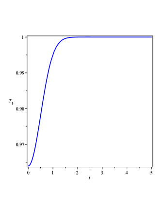
Figure 1: Qualitative behavior of the first order torsion scalar perturbation versus time for radiation matter with vanishing energy-momentum scalar. $T^{\prime}_{1}$ will reach a constant value given by $q/p$ and so the matter in this scenario is always stable.

4 Conclusion

From a geometric point of view, modifying gravity seems a necessary task in order to explain recent positively accelerated expansion of the universe. Any such modified theory, whether it is in the context of general relativity or in teleparallel gravity, may be expected to show some strong deviation from the standard gravity at very high energies and in strong-field regimes. This is because we still do not have a proper theory of quantum gravity to describe the behavior of gravitational interactions at those energies. On the other hand any strong deviation from the standard gravity at low energies and weak-field regimes immediately disqualify the theory because it will contradicts well established weak-field experiments. One of these experiments is the stability of weak-field celestial bodies or any other weak gravity objects. In this paper we’ve investigated the stability of such objects in the context of modified teleparallel gravity. The analysis shows that there is no Dolgov-Kawasaki matter instability in these type of theories. In contrast, in the corresponding $f(R)$ theories a certain stability condition should be met. This gives a great advantage to $f(T)$ theories over their $f(R)$ counterparts because from matter stability viewpoint, there is no limit on the form of functions that can be chosen to replace the torsion scalar in the action of $f(T)$ theories. We note that we have extended our analysis to the second order of perturbations and we have observed that the matter is still stable in this scenario.

Appendix A

Here we present the proof of equation (23) for an almost flat region inside a weak field gravitational body. For such an object the tetrad and metric are given by equations (18) and (20) respectively. Considering only the first order perturbations and dropping the subscript we have the following equations for the torsion and superpotential tensors

$$T_{\,\,\,\,\mu\nu}^{\rho}=\partial_{\mu}\tilde{e}_{\nu}^{\,\,\rho}-\partial_{\nu}\tilde{e}_{\mu}^{\,\,\rho}$$ (32)

and

$$S^{\,\,\,\,\rho\mu}_{\nu}=\partial^{\rho}\tilde{e}_{\nu}^{\,\,\mu}-\partial^{\mu}\tilde{e}_{\nu}^{\,\,\rho}-\delta_{\nu}^{\mu}(\partial^{\rho}\tilde{e}_{\sigma}^{\,\,\sigma}-\partial_{\sigma}\tilde{e}^{\sigma\rho})$$

$$+\delta_{\nu}^{\rho}(\partial^{\mu}\tilde{e}_{\sigma}^{\,\,\sigma}-\partial_{\sigma}\tilde{e}^{\sigma\mu})$$ (33)

the tensor $\tilde{e}_{\nu}^{\,\,\mu}$ is not necessarily symmetric but it has been shown that the anti-symmetric part of it has no physical significance in the field equations so we assume it to be symmetric here[4]. Furthermore for an almost flat region inside a star, we can safely assume that both the background and the first order correction are homogeneous and isotropic. In that case the torsion and its perturbation does not depend on spatial coordinates and we have $\partial_{\mu}\rightarrow\partial_{t}$. Also for a homogeneous and isotropic perturbation the first order correction of the tetrad has the form

$$\tilde{e}_{\nu}^{\,\,\mu}=diag(1,b,b,b)$$ (34)

and $b$ only depends on time. Substituting this in (A1) and (A2), we can find the torsion scalar as

$$T=S^{\rho\mu\nu}T_{\rho\mu\nu}=-6\dot{b}^{2}$$ (35)

Up to the first order in perturbations, the second term in the R.H.S of Eq. (16) will be $\nabla_{\mu}T_{\nu}^{\,\,\,\mu\nu}=3\ddot{b}$. On the other hand the only non zero components of the superpotential tensor are all the same (up to a sign) and proportional to $\sqrt{T}$, in particular we have

$$\partial_{\mu}S_{\nu}^{\mu\nu}=\frac{3}{2}\ddot{b}$$ (36)

so we will have the relation

$$\partial_{\mu}S_{\nu}^{\mu\nu}=\frac{3}{2\sqrt{6}}\partial_{t}{(\sqrt{-T})}$$ (37)

substituting from (16), equation (23) is obtained.

References

- [1] A. Einstein, Math. Annal. 102, 685 (1930). For an english translation, see A. Unzicker and T. Case, [arXiv:physics/0503046v1].
- [2] R. Weitzenbock, Invariance Theorie, Nordhoff, Groningen, 1923.
- [3] K. Hayashi and T. Shirafuji, Phys. Rev. D 19, 3524 (1979); K. Hayashi and T. Shirafuji, Phys. Rev. D 24, 3312 (1981);
- [4] R.Aldrovandi and J. G. Pereira, An Introduction to Teleparallel Gravity, Instituto de Fisica Teorica, UNSEP, Sao Paulo.
- [5] A. G. Riess et al. [Supernova Search Team Collaboration], Astron. J. 116, 1009 (1998); S. Perlmutter et al. [Supernova Cosmology Project Collaboration], Astrophys. J. 517, 565 (1999);
- [6] S. M. Carroll, V. Duvvuri, M. Trodden and M. S. Turner, Phys. Rev. D 70, 043528 (2004); S. Nojiri and S. D. Odintsov, Gen. Rel. Grav. 36, 1765 (2004); S. Nojiri and S. D. Odintsov, Phys. Rev. D 68, 123512 (2003); G. Allemandi, M. Capone, S. Capozziello and M. Francaviglia, Gen. Rel. Grav. 38, 33 (2006); S. Nojiri and S.D. Odintsov, [arXiv:hep-th/0601213]; T. P. Sotiriou, Class. Quant. Grav. 23, 5117 (2006); T. P. Sotiriou and S. Liberati, Annals Phys. 322, 935 (2007); T. P. Sotiriou and V. Faraoni, Rev. Mod. Phys. 82, 451 (2010); S. Tsujikawa, Lect. Notes Phys. 800, 99 (2010); S. Nojiri and S. D. Odintsov, Phys. Rept. 505, 59 (2011).
- [7] R. Ferraro and F. Fiorini, Phys. Rev. D75, 084031 (2007); R. Ferraro and F. Fiorini, Phys. Rev. D78, 124019 (2008); P. Wu and H. W. Yu, Eur. Phys. J. C 71, 1552 (2011); R. Zheng and Q. G. Huang, JCAP 1103, 002 (2011); K. Bamba, C. Q. Geng, C. C. Lee and L. W. Luo, JCAP 1101, 021 (2011); T. Wang, Phys. Rev. D84, 024042 (2011); P. Wu and H. W. Yu, Phys. Lett. B 693, 415 (2010); G. R. Bengochea, Phys. Lett. B 695, 405 (2011); P. Wu and H. W. Yu, Phys. Lett. B692, 176 (2010); S. H. Chen, J. B. Dent, S. Dutta and E. N. Saridakis, Phys. Rev. D 83, 023508 (2011); J. B. Dent, S. Dutta and E. N. Saridakis, JCAP 1101, 009 (2011); X. C. Ao, X. Z. Li and P. Xi, Phys. Lett. B694, 186 (2010); Y. Zhang, H. Li, Y. Gong and Z. H. Zhu, JCAP 1107, 015 (2011); R. Ferraro and F. Fiorini, Phys. Lett. B702, 75 (2011); H. Wei, X. P. Ma and H. Y. Qi, Phys. Lett. B703, 74 (2011); P. Wu and H. Yu, Phys. Lett. B703, 223 (2011); C. Q. Geng, C. C. Lee, E. N. Saridakis, Y. P. Wu, Phys. Lett. B704, 384 (2011); S. Capozziello, V. F. Cardone, H. Farajollahi and A. Ravanpak, Phys. Rev. D 84, 043527 (2011); K. Karami and A. Abdolmaleki, JCAP 04, 007 (2012); M. Li, R. -X. Miao, Y. -G. Miao, JHEP 1107, 108 (2011); R. -X. Miao, M. Li and Y. -G. Miao, JCAP 11, 033 (2011).
- [8] G. R. Bengochea and R. Ferraro, Phys. Rev. D 79, 124019 (2009).
- [9] E. V. Linder, Phys. Rev. D 81, 127301 (2010).
- [10] B. Li, T. P. Sotiriou and J. D. Barrow, Phys. Rev. D 83, 064035 (2011).
- [11] A. D. Dolgov and M. Kawasaki, Phys. Lett. B 573, 1 (2003).
- [12] V. Faraoni, Phys. Rev. D 74 104017 (2006)