Sparse Signal Separation in Redundant Dictionaries

Abstract

We formulate a unified framework for the separation of signals that are sparse in “morphologically” different redundant dictionaries. This formulation incorporates the so-called “analysis” and “synthesis” approaches as special cases and contains novel hybrid setups. We find corresponding coherence-based recovery guarantees for an $\ell_{1}$-norm based separation algorithm. Our results recover those reported in Studer and Baraniuk, ACHA, submitted, for the synthesis setting, provide new recovery guarantees for the analysis setting, and form a basis for comparing performance in the analysis and synthesis settings. As an aside our findings complement the D-RIP recovery results reported in Candès et al., ACHA, 2011, for the “analysis” signal recovery problem

$$\underset{\widetilde{\mathbf{x}}}{\text{minimize}}\,\,\|\boldsymbol{\Psi}\widetilde{\mathbf{x}}\|_{1}\quad\text{subject to}\,\,\|\mathbf{y}-\mathbf{A}\widetilde{\mathbf{x}}\|_{2}\leq\varepsilon$$

by delivering corresponding coherence-based recovery results.

I Introduction

We consider the problem of splitting the signal $\mathbf{x}=\mathbf{x}_{1}+\mathbf{x}_{2}$ into its constituents $\mathbf{x}_{1}\in\mathbb{C}^{d}$ and $\mathbf{x}_{2}\in\mathbb{C}^{d}$—assumedto be sparse in “morphologically” different (redundant) dictionaries [1]—based on $m$ linear, nonadaptive, and noisy measurements $\mathbf{y}=\mathbf{A}\mathbf{x}+\mathbf{e}$. Here, $\mathbf{A}\in\mathbb{C}^{m\times d}$, $m\leq d$, is the measurement matrix, assumed to be known, and $\mathbf{e}\in\mathbb{C}^{m}$ is a noise vector, assumed to be unknown and to satisfy $\|\mathbf{e}\|_{2}\leq\varepsilon$, with $\varepsilon$ known.

Redundant dictionaries [2, 3] often lead to sparser representations than nonredundant ones, such as, e.g., orthonormal bases, and have therefore become pervasive in the sparse signal recovery literature [3]. In the context of signal separation, redundant dictionaries lead to an interesting dichotomy [4, 1, 5]:

• In the so-called “synthesis” setting, it is assumed that, for $\ell=1,2$, $\mathbf{x}_{\ell}=\mathbf{D}_{\ell}\mathbf{s}_{\ell}$, where $\mathbf{D}_{\ell}\in\mathbb{C}^{d\times n}$ ($d<n$) is a redundant dictionary (of full rank) and the coefficient vector $\mathbf{s}_{\ell}\in\mathbb{C}^{n}$ is sparse (or approximately sparse in the sense of [6]). Given the vector $\mathbf{y}\in\mathbb{C}^{m}$, the problem of finding the constituents $\mathbf{x}_{1}$ and $\mathbf{x}_{2}$ is formalized as [7]:

  $$(\text{PS})\left\{\begin{array}[]{ll}\displaystyle\operatorname*{minimize}_{\mathbf{\tilde{s}}_{1},\mathbf{\tilde{s}}_{2}}&\|\mathbf{\tilde{s}}_{1}\|_{1}+\|\mathbf{\tilde{s}}_{2}\|_{1}\\ \operatorname{subject\ to}&\|\mathbf{y}-\mathbf{A}(\mathbf{D}_{1}\mathbf{\tilde{s}}_{1}+\mathbf{D}_{2}\mathbf{\tilde{s}}_{2})\|_{2}\leq\varepsilon.\end{array}\right.$$

• In the so-called “analysis” setting, it is assumed that, for $\ell=1,2$, there exists a matrix $\boldsymbol{\Psi}_{\ell}\in\mathbb{C}^{n\times d}$ such that $\boldsymbol{\Psi}_{\ell}\mathbf{x}_{\ell}$ is sparse (or approximately sparse). The problem of recovering $\mathbf{x}_{1}$ and $\mathbf{x}_{2}$ from $\mathbf{y}$ is formalized as [5]:

  $$(\text{PA})\left\{\begin{array}[]{ll}\underset{\widetilde{\mathbf{x}}_{1},\widetilde{\mathbf{x}}_{2}}{\operatorname*{minimize}}&\|\boldsymbol{\Psi}_{1}\widetilde{\mathbf{x}}_{1}\|_{1}+\|\boldsymbol{\Psi}_{2}\widetilde{\mathbf{x}}_{2}\|_{1}\\ \operatorname{subject\ to}&\|\mathbf{y}-\mathbf{A}(\widetilde{\mathbf{x}}_{1}+\widetilde{\mathbf{x}}_{2})\|_{2}\leq\varepsilon.\end{array}\right.$$

Throughout the paper, we exclusively consider redundant dictionaries as for $\mathbf{D}_{\ell}$, $\ell=1,2$, square, the synthesis setting can be recovered from the analysis setting by taking $\boldsymbol{\Psi}_{\ell}=\mathbf{D}_{\ell}^{-1}$.

The problems $(\text{PS})$ and $(\text{PA})$ arise in numerous applications including denoising [8], super-resolution [8], inpainting [9, 10, 11], deblurring [11], and recovery of sparsely corrupted signals [12]. Coherence-based recovery guarantees for $(\text{PS})$ were reported in [7]. The problem $(\text{PA})$ was mentioned in [5]. In the noiseless case, recovery guarantees for $(\text{PA})$, expressed in terms of a concentration inequality, are given in [13] for $\mathbf{A}=\mathbf{I}_{d}$ and $\boldsymbol{\Psi}_{1}$ and $\boldsymbol{\Psi}_{2}$ both Parseval frames [2].

Contributions

We consider the general problem

$$(\text{P})\left\{\begin{array}[]{ll}\underset{\widetilde{\mathbf{x}}_{1},\widetilde{\mathbf{x}}_{2}}{\operatorname*{minimize}}&\|\boldsymbol{\Psi}_{1}\widetilde{\mathbf{x}}_{1}\|_{1}+\|\boldsymbol{\Psi}_{2}\widetilde{\mathbf{x}}_{2}\|_{1}\\ \operatorname{subject\ to}&\|\mathbf{y}-\mathbf{A}_{1}\widetilde{\mathbf{x}}_{1}-\mathbf{A}_{2}\widetilde{\mathbf{x}}_{2}\|_{2}\leq\varepsilon,\end{array}\right.$$

which encompasses $(\text{PS})$ and $(\text{PA})$. To recover $(\text{PS})$ from (P), one sets $\mathbf{A}_{\ell}=\mathbf{A}\mathbf{D}_{\ell}$ and $\boldsymbol{\Psi}_{\ell}=[\mathbf{I}_{d}\ \mathbf{0}_{d,n-d}]^{T}$, for $\ell=1,2$. $(\text{PA})$ is obtained by choosing $\mathbf{A}_{\ell}=\mathbf{A}$, for $\ell=1,2$. Our main contribution is a coherence-based recovery guarantee for the general problem $(\text{P})$. This result recovers [7, Th. 4], which deals with $(\text{PS})$, provides new recovery guarantees for $(\text{PA})$, and constitutes a basis for comparing performance in the analysis and synthesis settings. As an aside, it also complements the D-RIP recovery guarantee in [5, Th. 1.2] for the problem

$$(\text{P}^{*})\,\,\,\underset{\widetilde{\mathbf{x}}}{\operatorname*{minimize}}\,\,\|\boldsymbol{\Psi}\widetilde{\mathbf{x}}\|_{1}\quad\operatorname{subject\ to}\,\,\|\mathbf{y}-\mathbf{A}\widetilde{\mathbf{x}}\|_{2}\leq\varepsilon$$

by delivering a corresponding coherence-based recovery guarantee. Moreover, the general formulation $(\text{P})$ encompasses novel hybrid problems of the form

$$\begin{array}[]{ll}\underset{\mathbf{\tilde{s}}_{1},\widetilde{\mathbf{x}}_{2}}{\operatorname*{minimize}}&\|\mathbf{\tilde{s}}_{1}\|_{1}+\|\boldsymbol{\Psi}_{2}\widetilde{\mathbf{x}}_{2}\|_{1}\\ \operatorname{subject\ to}&\|\mathbf{y}-\mathbf{A}(\mathbf{D}_{1}\mathbf{\tilde{s}}_{1}-\widetilde{\mathbf{x}}_{2})\|_{2}\leq\varepsilon.\end{array}$$

(a) Original cartoon image

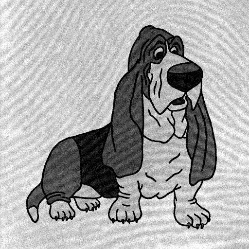
(b) Corrupted image

(c) Restored cartoon image

Figure 1: Image separation in the presence of Gaussian noise ($\text{SNR}=20\,\text{dB}$).

Notation

Lowercase boldface letters stand for column vectors and uppercase boldface letters denote matrices. The transpose, conjugate transpose, and Moore-Penrose inverse of the matrix $\mathbf{M}$ are designated as $\mathbf{M}^{T}$, $\mathbf{M}^{H}$, and $\mathbf{M}^{\dagger}$, respectively. The $j$th column of $\mathbf{M}$ is written $[\mathbf{M}]_{j}$, and the entry in the $i$th row and $j$th column of $\mathbf{M}$ is $[\mathbf{M}]_{i,j}$. We let $\sigma_{\text{min}}(\mathbf{M})$ denote the smallest singular value of $\mathbf{M}$, use $\mathbf{I}_{n}$ for the $n\times n$ identity matrix, and let $\mathbf{0}_{k\times m}$ be the $k\times m$ all zeros matrix. For matrices $\mathbf{M}$ and $\mathbf{N}$, we let $\omega_{\text{min}}(\mathbf{M})\triangleq\min_{j}\|[\mathbf{M}]_{j}\|_{2}$, $\omega_{\text{max}}(\mathbf{M})\triangleq\max_{j}\|[\mathbf{M}]_{j}\|_{2}$, $\omega_{\text{min}}(\mathbf{M},\mathbf{N})\triangleq\min\{\omega_{\text{min}}(\mathbf{M}),\omega_{\text{min}}(\mathbf{N})\}$, and $\omega_{\text{max}}(\mathbf{M},\mathbf{N})\triangleq\max\{\omega_{\text{max}}(\mathbf{M}),\omega_{\text{max}}(\mathbf{N})\}$. The $k$th entry of the vector $\mathbf{x}$ is written $[\mathbf{x}]_{k}$, and $\|\mathbf{x}\|_{1}\triangleq\sum_{k}|[\mathbf{x}]_{k}|$ stands for its $\ell_{1}$-norm. We take $\text{supp}_{k}(\mathbf{x})$ to be the set of indices corresponding to the $k$ largest (in magnitude) coefficients of $\mathbf{x}$. Sets are designated by uppercase calligraphic letters; the cardinality of the set $\mathcal{S}$ is $|\mathcal{S}|$ and the complement of $\mathcal{S}$ (in some given set) is denoted by $\mathcal{S}^{c}$. For a set $\mathcal{S}$ of integers and $n\in\mathbb{Z}$, we let $n+\mathcal{S}\triangleq\{n+p:p\in\mathcal{S}\}$. The $n\times n$ diagonal projection matrix $\mathbf{P}_{\mathcal{S}}$ for the set $\mathcal{S}\subset\{1,\ldots,n\}$ is defined as follows:

$$[\mathbf{P}_{\mathcal{S}}]_{i,j}=\left\{\begin{array}[]{ll}1,&i=j\text{ and }i\in\mathcal{S}\\ 0,&\text{otherwise,}\end{array}\right.$$

and we set $\mathbf{M}_{\mathcal{S}}\triangleq\mathbf{P}_{\mathcal{S}}\mathbf{M}$. We define $\sigma_{k}(\mathbf{x})$ to be the $\ell_{1}$-norm approximation error of the best $k$-sparse approximation of $\mathbf{x}$, i.e., $\sigma_{k}(\mathbf{x})\triangleq\|\mathbf{x}-\mathbf{x}_{\mathcal{S}}\|_{1}$ where $\mathcal{S}=\text{supp}_{k}(\mathbf{x})$ and $\mathbf{x}_{\mathcal{S}}\triangleq\mathbf{P}_{\mathcal{S}}\mathbf{x}$.

II Recovery Guarantees

Coherence definitions in the sparse signal recovery literature [3] usually apply to dictionaries with normalized columns. Here, we will need coherence notions valid for general (unnormalized) dictionaries $\mathbf{M}$ and $\mathbf{N}$, assumed, for simplicity of exposition, to consist of nonzero columns only.

Definition 1 (Coherence)

The coherence of the dictionary $\mathbf{M}$ is defined as

$$\hat{\mu}(\mathbf{M})=\underset{i,j,i\neq j}{\max}\,\,\frac{|[\mathbf{M}^{H}\mathbf{M}]_{i,j}|}{\omega_{\text{min}}^{2}(\mathbf{M})}.$$ (1)

Definition 2 (Mutual coherence)

The mutual coherence of the dictionaries $\mathbf{M}$ and $\mathbf{N}$ is defined as

$$\hat{\mu}_{m}(\mathbf{M},\mathbf{N})=\underset{i,j}{\max}\,\,\frac{|[\mathbf{M}^{H}\mathbf{N}]_{i,j}|}{\omega_{\text{min}}^{2}(\mathbf{M},\mathbf{N})}.$$ (2)

The main contribution of this paper is the following recovery guarantee for $(\text{P})$.

Theorem 1

Let $\mathbf{y}=\mathbf{A}_{1}\mathbf{x}_{1}+\mathbf{A}_{2}\mathbf{x}_{2}+\mathbf{e}$ with $\|\mathbf{e}\|_{2}\leq\varepsilon$ and let $\boldsymbol{\Psi}_{1}\in\mathbb{C}^{n_{1}\times p_{1}}$ and $\boldsymbol{\Psi}_{2}\in\mathbb{C}^{n_{2}\times p_{2}}$ be full-rank matrices. Let $\mathbf{x}=[\mathbf{x}_{1}^{T}\ \mathbf{x}_{2}^{T}]^{T}$, $\hat{\mu}_{1}=\hat{\mu}(\mathbf{A}_{1}\boldsymbol{\Psi}_{1}^{\dagger})$, $\hat{\mu}_{2}=\hat{\mu}(\mathbf{A}_{2}\boldsymbol{\Psi}_{2}^{\dagger})$, $\hat{\mu}_{m}=\hat{\mu}_{m}(\mathbf{A}_{1}\boldsymbol{\Psi}_{1}^{\dagger},\mathbf{A}_{2}\boldsymbol{\Psi}_{2}^{\dagger})$, and $\hat{\mu}_{\text{max}}=\max\{\hat{\mu}_{1},\hat{\mu}_{2},\hat{\mu}_{m}\}$. Without loss of generality, we assume that $\hat{\mu}_{1}\leq\hat{\mu}_{2}$. Let $k_{1}$ and $k_{2}$ be nonnegative integers such that

$$k_{1}+k_{2}<\max\left\{\frac{2(1+\hat{\mu}_{2})}{\hat{\mu}_{2}+2\hat{\mu}_{\text{max}}+\sqrt{\hat{\mu}_{2}^{2}+\hat{\mu}_{m}^{2}}},\frac{1+\hat{\mu}_{\text{max}}}{2\hat{\mu}_{\text{max}}}\right\}.$$ (3)

Then, the solution $(\mathbf{x}_{1}^{*},\,\mathbf{x}_{2}^{*})$ to the convex program $(\text{P})$ satisfies

$$\|\mathbf{x}^{*}-\mathbf{x}\|_{2}\leq C_{0}\,\varepsilon+C_{1}\!\left(\sigma_{k_{1}}(\boldsymbol{\Psi}_{1}\mathbf{x}_{1})+\sigma_{k_{2}}(\boldsymbol{\Psi}_{2}\mathbf{x}_{2})\right),$$ (4)

where $C_{0},C_{1}\geq 0$ are constants that do not depend on $\mathbf{x}_{1}$ and $\mathbf{x}_{2}$ and where $\mathbf{x}^{*}=[{\mathbf{x}_{1}^{*}}^{T}\ {\mathbf{x}_{2}^{*}}^{T}]^{T}$.

Note that the quantities $\hat{\mu}_{1}$, $\hat{\mu}_{2}$, and $\hat{\mu}_{m}$ characterize the interplay between the measurement matrix $\mathbf{A}$ and the sparsifying transforms $\boldsymbol{\Psi}_{1}$ and $\boldsymbol{\Psi}_{2}$.

As a corollary to our main result, we get the following statement for the problem $(\text{P}^{*})$ considered in [5].

Corollary 2

Let $\mathbf{y}=\mathbf{A}\mathbf{x}+\mathbf{e}$ with $\|\mathbf{e}\|_{2}\leq\varepsilon$ and let $\boldsymbol{\Psi}\in\mathbb{C}^{n\times p}$ be a full-rank matrix. Let $k$ be a nonnegative integer such that

$$k<\frac{1}{2}\!\left(1+\frac{1}{\hat{\mu}(\mathbf{A}\boldsymbol{\Psi}^{\dagger})}\right).$$ (5)

Then, the solution $\mathbf{x}^{*}$ to the convex program $(\text{P}^{*})$ satisfies

$$\|\mathbf{x}^{*}-\mathbf{x}\|_{2}\leq C_{0}\,\varepsilon+C_{1}\sigma_{k}(\boldsymbol{\Psi}\mathbf{x}),$$ (6)

where $C_{0},C_{1}\geq 0$ are constants that do not depend on $\mathbf{x}$.

The proofs of Theorem 1 and Corollary 1 can be found in the Appendix.

We conclude by noting that D-RIP recovery guarantees for $(\text{P}^{*})$ were provided in [5]. As is common in RIP-based recovery guarantees the restricted isometry constants are, in general, hard to compute. Moreover, the results in [5] hinge on the assumption that $\boldsymbol{\Psi}$ forms a Parseval frame, i.e., $\boldsymbol{\Psi}^{H}\boldsymbol{\Psi}=\mathbf{I}_{d}$; a corresponding extension to general $\boldsymbol{\Psi}$ was provided in [14]. We finally note that it does not seem possible to infer the coherence-based threshold (5) from the D-RIP recovery guarantees in [5, 14].

III Numerical Results

We analyze an image-separation problem where we remove a fingerprint from a cartoon image. We corrupt the $512\times 512$ greyscale cartoon image depicted in Fig. 1(a) by adding a fingerprint and i.i.d. zero-mean Gaussian noise.

Cartoon images are constant apart from (a small number of) discontinuities and are thus sparse under the finite difference operator $\boldsymbol{\Delta}$ defined in [15]. Fingerprints are sparse under the application of a wave atom transform, $\mathbf{W}$, such as the redundancy $2$ transform available in the WaveAtom toolbox [16]. It is therefore sensible to perform separation by solving the problem $(\text{PA})$ with $\boldsymbol{\Psi}_{1}=\boldsymbol{\Delta}$, $\boldsymbol{\Psi}_{2}=\mathbf{W}$, and $\mathbf{A}=\mathbf{I}_{d}$. For our simulation, we use a regularized version of $\boldsymbol{\Delta}$ and we employ the TFOCS solver from [17].

Fig. 1(c) shows the corresponding recovered image. We can see that the restoration procedure gives visually satisfactory results.

Appendix A Proofs

For simplicity of exposition, we first present the proof of Corollary 1 and then describe the proof of Theorem 1.

A-A Proof of Corollary 1

We define the vector $\mathbf{h}=\mathbf{x}^{*}-\mathbf{x}$, where $\mathbf{x}^{*}$ is the solution to $(\text{P}^{*})$ and $\mathbf{x}$ is the vector to be recovered. We furthermore set $\mathcal{S}=\text{supp}_{k}(\boldsymbol{\Psi}\mathbf{x})$.

A-A1 Prerequisites

Our proof relies partly on two important results developed earlier in [5], [6] and summarized, for completeness, next.

Lemma 3 (Cone constraint ​​​[5],​ [6])

The vector $\boldsymbol{\Psi}\mathbf{h}$ obeys

$$\|\boldsymbol{\Psi}_{\mathcal{S}^{c}}\mathbf{h}\|_{1}\leq\|\boldsymbol{\Psi}_{\mathcal{S}}\mathbf{h}\|_{1}+2\|\boldsymbol{\Psi}_{\mathcal{S}^{c}}\mathbf{x}\|_{1},$$ (7)

where $\mathcal{S}=\text{supp}_{k}(\boldsymbol{\Psi}\mathbf{x})$.

Proof:

Since $\mathbf{x}^{*}$ is the minimizer of $(\text{P}^{*})$, the inequality $\|\boldsymbol{\Psi}\mathbf{x}\|_{1}\geq\|\boldsymbol{\Psi}\mathbf{x}^{*}\|_{1}$ holds. Using $\boldsymbol{\Psi}=\boldsymbol{\Psi}_{\mathcal{S}}+\boldsymbol{\Psi}_{\mathcal{S}^{c}}$ and $\mathbf{x}^{*}=\mathbf{x}+\mathbf{h}$, we obtain

$$\|\boldsymbol{\Psi}_{\mathcal{S}}\mathbf{x}\|_{1}+\|\boldsymbol{\Psi}_{\mathcal{S}^{c}}\mathbf{x}\|_{1}=\|\boldsymbol{\Psi}\mathbf{x}\|_{1}$$

$$\quad\geq\|\boldsymbol{\Psi}\mathbf{x}^{*}\|_{1}=\|\boldsymbol{\Psi}_{\mathcal{S}}\mathbf{x}+\boldsymbol{\Psi}_{\mathcal{S}}\mathbf{h}\|_{1}+\|\boldsymbol{\Psi}_{\mathcal{S}^{c}}\mathbf{x}+\boldsymbol{\Psi}_{\mathcal{S}^{c}}\mathbf{h}\|_{1}$$

$$\quad\geq\|\boldsymbol{\Psi}_{\mathcal{S}}\mathbf{x}\|_{1}-\|\boldsymbol{\Psi}_{\mathcal{S}}\mathbf{h}\|_{1}+\|\boldsymbol{\Psi}_{\mathcal{S}^{c}}\mathbf{h}\|_{1}-\|\boldsymbol{\Psi}_{\mathcal{S}^{c}}\mathbf{x}\|_{1}.$$

We retrieve (7) by simple rearrangement of terms. ∎

Lemma 4 (Tube constraint ​​​[5],​ [6])

The vector $\mathbf{A}\mathbf{h}$ satisfies $\|\mathbf{A}\mathbf{h}\|_{2}\leq 2\varepsilon$.

Proof:

Since both $\mathbf{x}^{*}$ and $\mathbf{x}$ are feasible (we recall that $\mathbf{y}=\mathbf{A}\mathbf{x}+\mathbf{e}$ with $\|\mathbf{e}\|_{2}\leq\varepsilon$), we have the following

$$\|\mathbf{A}\mathbf{h}\|_{2} =\|\mathbf{A}(\mathbf{x}^{*}-\mathbf{x})\|_{2}$$

$$\leq\|\mathbf{A}\mathbf{x}^{*}-\mathbf{y}\|_{2}+\|\mathbf{y}-\mathbf{A}\mathbf{x}\|_{2}\leq 2\varepsilon,$$

thus establishing the lemma. ∎

A-A2 Bounding the recovery error

We want to bound $\|\mathbf{h}\|_{2}$ from above. Since $\sigma_{\text{min}}(\boldsymbol{\Psi})>0$ by assumption ($\boldsymbol{\Psi}$ is assumed to be full-rank), it follows from the Rayleigh-Ritz theorem [18, Th. 4.2.2] that

$$\|\mathbf{h}\|_{2}\leq\frac{1}{\sigma_{\text{min}}(\boldsymbol{\Psi})}\|\boldsymbol{\Psi}\mathbf{h}\|_{2}.$$ (9)

We now set $\mathcal{Q}=\text{supp}_{k}(\boldsymbol{\Psi}\mathbf{h})$. Clearly, we have for $i\in\mathcal{Q}^{c}$,

$$|[\boldsymbol{\Psi}\mathbf{h}]_{i}|\leq\frac{\|\boldsymbol{\Psi}_{\mathcal{Q}}\mathbf{h}\|_{1}}{k}.$$

Using the same argument as in [19, Th. 3.1], we obtain

$$\|\boldsymbol{\Psi}_{\mathcal{Q}^{c}}\mathbf{h}\|_{2}^{2}=\sum_{i\in\mathcal{Q}^{c}}|[\boldsymbol{\Psi}\mathbf{h}]_{i}|^{2} \leq\sum_{i\in\mathcal{Q}^{c}}|[\boldsymbol{\Psi}\mathbf{h}]_{i}|\frac{\|\boldsymbol{\Psi}_{\mathcal{Q}}\mathbf{h}\|_{1}}{k}$$

$$=\|\boldsymbol{\Psi}_{\mathcal{Q}^{c}}\mathbf{h}\|_{1}\frac{\|\boldsymbol{\Psi}_{\mathcal{Q}}\mathbf{h}\|_{1}}{k}.$$ (10)

Since $\mathcal{Q}$ is the set of indices of the $k$ largest (in magnitude) coefficients of $\boldsymbol{\Psi}\mathbf{h}$ and since $\mathcal{Q}$ and $\mathcal{S}$ both contain $k$ elements, we have $\|\boldsymbol{\Psi}_{\mathcal{S}}\mathbf{h}\|_{1}\leq\|\boldsymbol{\Psi}_{\mathcal{Q}}\mathbf{h}\|_{1}$ and $\|\boldsymbol{\Psi}_{\mathcal{Q}^{c}}\mathbf{h}\|_{1}\leq\|\boldsymbol{\Psi}_{\mathcal{S}^{c}}\mathbf{h}\|_{1}$, which, combined with the cone constraint in Lemma 3, yields

$$\|\boldsymbol{\Psi}_{\mathcal{Q}^{c}}\mathbf{h}\|_{1}\leq\|\boldsymbol{\Psi}_{\mathcal{Q}}\mathbf{h}\|_{1}+2\|\boldsymbol{\Psi}_{\mathcal{S}^{c}}\mathbf{x}\|_{1}.$$ (11)

The inequality in (10) then becomes

$$\|\boldsymbol{\Psi}_{\mathcal{Q}^{c}}\mathbf{h}\|_{2}^{2} \leq\frac{\|\boldsymbol{\Psi}_{\mathcal{Q}}\mathbf{h}\|_{1}^{2}}{k}+2\|\boldsymbol{\Psi}_{\mathcal{S}^{c}}\mathbf{x}\|_{1}\frac{\|\boldsymbol{\Psi}_{\mathcal{Q}}\mathbf{h}\|_{1}}{k}$$

$$\leq\|\boldsymbol{\Psi}_{\mathcal{Q}}\mathbf{h}\|_{2}^{2}+2\|\boldsymbol{\Psi}_{\mathcal{S}^{c}}\mathbf{x}\|_{1}\frac{\|\boldsymbol{\Psi}_{\mathcal{Q}}\mathbf{h}\|_{2}}{\sqrt{k}}$$ (12a)

$$\leq 2\|\boldsymbol{\Psi}_{\mathcal{Q}}\mathbf{h}\|_{2}^{2}+\frac{\|\boldsymbol{\Psi}_{\mathcal{S}^{c}}\mathbf{x}\|_{1}^{2}}{k},$$ (12b)

where (12a) follows from $\|\mathbf{u}\|_{1}\leq\sqrt{k}\|\mathbf{u}\|_{2}$ for $k$-sparse $\mathbf{u}$ and (12b) is a consequence of $2xy\leq x^{2}+y^{2}$, for $x,y\in\mathbb{R}$.

It now follows that

$$\|\boldsymbol{\Psi}\mathbf{h}\|_{2} =\sqrt{\|\boldsymbol{\Psi}_{\mathcal{Q}}\mathbf{h}\|_{2}^{2}+\|\boldsymbol{\Psi}_{\mathcal{Q}^{c}}\mathbf{h}\|_{2}^{2}}$$

$$\leq\sqrt{3\|\boldsymbol{\Psi}_{\mathcal{Q}}\mathbf{h}\|_{2}^{2}+\frac{\|\boldsymbol{\Psi}_{\mathcal{S}^{c}}\mathbf{x}\|_{1}^{2}}{k}}$$ (13a)

$$\leq\sqrt{3}\|\boldsymbol{\Psi}_{\mathcal{Q}}\mathbf{h}\|_{2}+\frac{\|\boldsymbol{\Psi}_{\mathcal{S}^{c}}\mathbf{x}\|_{1}}{\sqrt{k}},$$ (13b)

where (13a) is a consequence of (12b) and (13b) results from $\sqrt{x^{2}+y^{2}}\leq x+y$, for $x,y\geq 0$.

Combining (9) and (13b) leads to

$$\|\mathbf{h}\|_{2}\leq\frac{1}{\sigma_{\text{min}}(\boldsymbol{\Psi})}\!\left(\sqrt{3}\|\boldsymbol{\Psi}_{\mathcal{Q}}\mathbf{h}\|_{2}+\frac{\|\boldsymbol{\Psi}_{\mathcal{S}^{c}}\mathbf{x}\|_{1}}{\sqrt{k}}\right).$$ (14)

A-A3 Bounding the term $\|\boldsymbol{\Psi}_{\mathcal{Q}}\mathbf{h}\|_{2}$ in (14)

In the last step of the proof, we bound the term $\|\boldsymbol{\Psi}_{\mathcal{Q}}\mathbf{h}\|_{2}$ in (14). To this end, we first bound $\|\mathbf{A}\boldsymbol{\Psi}^{\dagger}\boldsymbol{\Psi}_{\mathcal{Q}}\mathbf{h}\|_{2}^{2}$, with $\boldsymbol{\Psi}^{\dagger}=(\boldsymbol{\Psi}^{H}\boldsymbol{\Psi})^{-1}\boldsymbol{\Psi}^{H}$, using Geršgorin’s disc theorem [18, Th. 6.2.2]:

$$\theta_{\text{min}}\|\boldsymbol{\Psi}_{\mathcal{Q}}\mathbf{h}\|_{2}^{2}\leq\|\mathbf{A}\boldsymbol{\Psi}^{\dagger}\boldsymbol{\Psi}_{\mathcal{Q}}\mathbf{h}\|_{2}^{2}\leq\theta_{\text{max}}\|\boldsymbol{\Psi}_{\mathcal{Q}}\mathbf{h}\|_{2}^{2}$$ (15)

where $\theta_{\text{min}}\triangleq\omega_{\text{min}}^{2}-\mu(k-1)$ and $\theta_{\text{max}}\triangleq\omega_{\text{max}}^{2}+\mu(k-1)$ with

$$\mu=\underset{i,j,i\neq j}{\max}\,|[(\mathbf{A}\boldsymbol{\Psi}^{\dagger})^{H}\mathbf{A}\boldsymbol{\Psi}^{\dagger}]_{i,j}|$$ (16)

and $\omega_{\text{min}}\triangleq\omega_{\text{min}}(\mathbf{A}\boldsymbol{\Psi}^{\dagger})$ and $\omega_{\text{max}}\triangleq\omega_{\text{max}}(\mathbf{A}\boldsymbol{\Psi}^{\dagger})$.

Using Lemma 4 and (15) and following the same steps as in [20, Th. 2.1] and [7, Th. 1], we arrive at the following chain of inequalities:

$$\theta_{\text{min}}\|\boldsymbol{\Psi}_{\mathcal{Q}}\mathbf{h}\|_{2}^{2}\leq\|\mathbf{A}\boldsymbol{\Psi}^{\dagger}\boldsymbol{\Psi}_{\mathcal{Q}}\mathbf{h}\|_{2}^{2}=(\mathbf{A}\boldsymbol{\Psi}^{\dagger}\boldsymbol{\Psi}_{\mathcal{Q}}\mathbf{h})^{H}\mathbf{A}\boldsymbol{\Psi}^{\dagger}\boldsymbol{\Psi}_{\mathcal{Q}}\mathbf{h}$$

$$\!\!\!=(\mathbf{A}\mathbf{h})^{H}\mathbf{A}\boldsymbol{\Psi}^{\dagger}\boldsymbol{\Psi}_{\mathcal{Q}}\mathbf{h}-(\mathbf{A}\boldsymbol{\Psi}^{\dagger}\boldsymbol{\Psi}_{\mathcal{Q}^{c}}\mathbf{h})^{H}\mathbf{A}\boldsymbol{\Psi}^{\dagger}\boldsymbol{\Psi}_{\mathcal{Q}}\mathbf{h}$$ (17a)

$$\!\!\!\leq|(\mathbf{A}\mathbf{h})^{H}\mathbf{A}\boldsymbol{\Psi}^{\dagger}\boldsymbol{\Psi}_{\mathcal{Q}}\mathbf{h}|+|(\boldsymbol{\Psi}_{\mathcal{Q}^{c}}\mathbf{h})^{H}(\mathbf{A}\boldsymbol{\Psi}^{\dagger})^{H}\mathbf{A}\boldsymbol{\Psi}^{\dagger}(\boldsymbol{\Psi}_{\mathcal{Q}}\mathbf{h})|$$

$$\!\!\!\leq\|\mathbf{A}\mathbf{h}\|_{2}\|\mathbf{A}\boldsymbol{\Psi}^{\dagger}\boldsymbol{\Psi}_{\mathcal{Q}}\mathbf{h}\|_{2}$$

$$\qquad\,\,\,+\sum_{i\in\mathcal{Q}^{c},j\in\mathcal{Q}}|[(\mathbf{A}\boldsymbol{\Psi}^{\dagger})^{H}\mathbf{A}\boldsymbol{\Psi}^{\dagger}]_{i,j}||[\boldsymbol{\Psi}\mathbf{h}]_{i}||[\boldsymbol{\Psi}\mathbf{h}]_{j}|$$ (17b)

$$\!\!\!\leq 2\varepsilon\sqrt{\theta_{\text{max}}}\|\boldsymbol{\Psi}_{\mathcal{Q}}\mathbf{h}\|_{2}+\mu\|\boldsymbol{\Psi}_{\mathcal{Q}}\mathbf{h}\|_{1}\|\boldsymbol{\Psi}_{\mathcal{Q}^{c}}\mathbf{h}\|_{1}$$ (17c)

$$\!\!\!\leq 2\varepsilon\sqrt{\theta_{\text{max}}}\|\boldsymbol{\Psi}_{\mathcal{Q}}\mathbf{h}\|_{2}+\mu\|\boldsymbol{\Psi}_{\mathcal{Q}}\mathbf{h}\|_{1}\left(\|\boldsymbol{\Psi}_{\mathcal{Q}}\mathbf{h}\|_{1}+2\|\boldsymbol{\Psi}_{\mathcal{S}^{c}}\mathbf{x}\|_{1}\right)$$ (17d)

$$\!\!\!\leq 2\varepsilon\sqrt{\theta_{\text{max}}}\|\boldsymbol{\Psi}_{\mathcal{Q}}\mathbf{h}\|_{2}+\mu k\|\boldsymbol{\Psi}_{\mathcal{Q}}\mathbf{h}\|_{2}^{2}$$

$$\qquad\,\,\,+2\mu\sqrt{k}\|\boldsymbol{\Psi}_{\mathcal{S}^{c}}\mathbf{x}\|_{1}\|\boldsymbol{\Psi}_{\mathcal{Q}}\mathbf{h}\|_{2},$$ (17e)

where (17a) follows from $\boldsymbol{\Psi}_{\mathcal{Q}}\mathbf{h}=\boldsymbol{\Psi}\mathbf{h}-\boldsymbol{\Psi}_{\mathcal{Q}^{c}}\mathbf{h}$ and $\boldsymbol{\Psi}^{\dagger}\boldsymbol{\Psi}=\mathbf{I}_{d}$, (17b) is a consequence of the Cauchy-Schwarz inequality, (17c) is obtained from (15), Lemma 4, and the definition of $\mu$ in (16), (17d) results from (11), and (17e) comes from $\|\mathbf{u}\|_{1}\leq\sqrt{k}\|\mathbf{u}\|_{2}$, for $k$-sparse $\mathbf{u}$.

If $\mathbf{h}\neq\mathbf{0}$, then $\|\boldsymbol{\Psi}_{\mathcal{Q}}\mathbf{h}\|_{2}\neq 0$, since $\boldsymbol{\Psi}$ is assumed to be full-rank and $\mathcal{Q}$ is the set of indices of the $k$ largest (in magnitude) coefficients of $\boldsymbol{\Psi}\mathbf{h}$, and therefore, the inequality between $\theta_{\text{min}}\|\boldsymbol{\Psi}_{\mathcal{Q}}\mathbf{h}\|_{2}^{2}$ and (17e) simplifies to

$$(\omega_{\text{min}}^{2}-\mu(2k-1))\|\boldsymbol{\Psi}_{\mathcal{Q}}\mathbf{h}\|_{2}\leq 2\varepsilon\sqrt{\theta_{\text{max}}}+2\mu\sqrt{k}\|\boldsymbol{\Psi}_{\mathcal{S}^{c}}\mathbf{x}\|_{1}.$$

This finally yields

$$\|\boldsymbol{\Psi}_{\mathcal{Q}}\mathbf{h}\|_{2}\leq\frac{2\varepsilon\sqrt{\theta_{\text{max}}}+2\mu\sqrt{k}\|\boldsymbol{\Psi}_{\mathcal{S}^{c}}\mathbf{x}\|_{1}}{\omega_{\text{min}}^{2}-\mu(2k-1)}$$ (18)

provided that

$$\omega_{\text{min}}^{2}-\mu(2k-1)>0.$$

A-A4 Recovery guarantee

Using Definition 1, we get $\hat{\mu}=\hat{\mu}(\mathbf{A}\boldsymbol{\Psi}^{\dagger})=\mu/\omega_{\text{min}}^{2}$. Combining (14) and (18), we therefore conclude that for

$$k<\frac{1}{2}\!\left(1+\frac{1}{\hat{\mu}}\right)$$ (19)

we have

$$\|\mathbf{x}^{*}-\mathbf{x}\|_{2}=\|\mathbf{h}\|_{2}\leq C_{0}\,\varepsilon+C_{1}\|\boldsymbol{\Psi}_{\mathcal{S}^{c}}\mathbf{x}\|_{1}$$

with

$$C_{0} =\frac{2\sqrt{3}}{\sigma_{\text{min}}(\boldsymbol{\Psi})\omega_{\text{min}}}\frac{\sqrt{\frac{\omega_{\text{max}}^{2}}{\omega_{\text{min}}^{2}}(1+\hat{\mu}(k-1)})}{1-\hat{\mu}(2k-1)}$$

$$C_{1} =\frac{1}{\sigma_{\text{min}}(\boldsymbol{\Psi})}\!\left(\frac{2\hat{\mu}\sqrt{3k}}{1-\hat{\mu}(2k-1)}+\frac{1}{\sqrt{k}}\right).$$

A-B Proof of Theorem 1

We start by transforming $(\text{P})$ into the equivalent problem

$$(\text{P}^{*})\,\,\,\underset{\widetilde{\mathbf{x}}}{\operatorname*{minimize}}\quad\|\boldsymbol{\Psi}\widetilde{\mathbf{x}}\|_{1}\quad\operatorname{subject\ to}\quad\|\mathbf{y}-\mathbf{A}\widetilde{\mathbf{x}}\|_{2}\leq\varepsilon$$

by amalgamating $\boldsymbol{\Psi}_{1},\boldsymbol{\Psi}_{2}$ and $\mathbf{A}_{1},\mathbf{A}_{2}$ into the matrices $\boldsymbol{\Psi}$ and $\mathbf{A}$ as follows:

$$\mathbf{A} =\begin{bmatrix}\mathbf{A}_{1}&\mathbf{A}_{2}\end{bmatrix}\in\mathbb{C}^{m\times p}$$ (20)

$$\boldsymbol{\Psi} =\begin{bmatrix}\boldsymbol{\Psi}_{1}&\mathbf{0}_{n\times d}\\ \mathbf{0}_{n\times d}&\boldsymbol{\Psi}_{2}\end{bmatrix}\in\mathbb{C}^{2n\times 2d},$$ (21)

where $p=2d$ in the analysis setting, $p=2n$ in the synthesis setting, and $p=d+n$ in hybrid settings. The corresponding measurement vector is $\mathbf{y}=\mathbf{A}\mathbf{x}+\mathbf{e}$, where we set $\mathbf{x}=[\mathbf{x}_{1}^{T}\ \mathbf{x}_{2}^{T}]^{T}$.

A recovery condition for $(\text{P})$ could now be obtained by simply inserting $\mathbf{A}$ and $\boldsymbol{\Psi}$ in (20), (21) above into (5). In certain cases, we can, however, get a better (i.e., less restrictive) threshold following ideas similar to those reported in [7] and detailed next.

We define the vectors $\mathbf{h}_{1}=\mathbf{x}_{1}^{*}-\mathbf{x}_{1}$, $\mathbf{h}_{2}=\mathbf{x}_{2}^{*}-\mathbf{x}_{2}$, the sets $\mathcal{Q}_{1}\triangleq\text{supp}_{k_{1}}(\boldsymbol{\Psi}_{1}\mathbf{h}_{1})$, $\mathcal{Q}_{2}\triangleq n+\text{supp}_{k_{2}}(\boldsymbol{\Psi}_{2}\mathbf{h}_{2})$, and $\mathbf{h}=[\mathbf{h}_{1}^{T}\ \mathbf{h}_{2}^{T}]^{T}$, $\mathcal{Q}=\mathcal{Q}_{1}\cup\mathcal{Q}_{2}$, and set $k=k_{1}+k_{2}$.

We furthermore let, for $\ell=1,2$,

$$\mu_{\ell}=\underset{i,j,i\neq j}{\max}\,|[(\mathbf{A}_{\ell}\boldsymbol{\Psi}_{\ell}^{\dagger})^{H}\mathbf{A}_{\ell}\boldsymbol{\Psi}_{\ell}^{\dagger}]_{i,j}|$$

$$\mu_{m}=\underset{i,j}{\max}\,|[(\mathbf{A}_{1}\boldsymbol{\Psi}_{1}^{\dagger})^{H}\mathbf{A}_{2}\boldsymbol{\Psi}_{2}^{\dagger}]_{i,j}|.$$

With the definitions of $\mathcal{Q}_{1}$ and $\mathcal{Q}_{2}$, we have from (15)

$$\|\mathbf{A}\boldsymbol{\Psi}^{\dagger}\boldsymbol{\Psi}_{\mathcal{Q}}\mathbf{h}\|_{2}^{2} =\|\mathbf{A}\boldsymbol{\Psi}^{\dagger}\boldsymbol{\Psi}_{\mathcal{Q}_{1}}\mathbf{h}\|_{2}^{2}+\|\mathbf{A}\boldsymbol{\Psi}^{\dagger}\boldsymbol{\Psi}_{\mathcal{Q}_{2}}\mathbf{h}\|_{2}^{2}$$

$$\qquad+2(\mathbf{A}\boldsymbol{\Psi}^{\dagger}\boldsymbol{\Psi}_{\mathcal{Q}_{1}}\mathbf{h})^{H}\mathbf{A}\boldsymbol{\Psi}^{\dagger}\boldsymbol{\Psi}_{\mathcal{Q}_{2}}\mathbf{h}.$$ (22)

The application of Geršgorin’s disc theorem [18] gives

$$\theta_{\text{min},1}\|\boldsymbol{\Psi}_{\mathcal{Q}_{1}}\mathbf{h}\|_{2}^{2}\leq\|\mathbf{A}\boldsymbol{\Psi}^{\dagger}\boldsymbol{\Psi}_{\mathcal{Q}_{1}}\mathbf{h}\|_{2}^{2}\leq\theta_{\text{max},1}\|\boldsymbol{\Psi}_{\mathcal{Q}_{1}}\mathbf{h}\|_{2}^{2}$$ (23)

$$\theta_{\text{min},2}\|\boldsymbol{\Psi}_{\mathcal{Q}_{2}}\mathbf{h}\|_{2}^{2}\leq\|\mathbf{A}\boldsymbol{\Psi}^{\dagger}\boldsymbol{\Psi}_{\mathcal{Q}_{2}}\mathbf{h}\|_{2}^{2}\leq\theta_{\text{max},2}\|\boldsymbol{\Psi}_{\mathcal{Q}_{2}}\mathbf{h}\|_{2}^{2}$$ (24)

with $\theta_{\text{min},\ell}\triangleq\omega_{\text{min}}^{2}(\mathbf{A}_{\ell}\boldsymbol{\Psi}_{\ell}^{\dagger})-\mu_{\ell}(k_{\ell}-1)$ and $\theta_{\text{max},\ell}\triangleq\omega_{\text{max}}^{2}(\mathbf{A}_{\ell}\boldsymbol{\Psi}_{\ell}^{\dagger})+\mu_{\ell}(k_{\ell}-1)$, for $\ell=1,2$.

In addition, the last term in (22) can be bounded as

$$|(\mathbf{A}\boldsymbol{\Psi}^{\dagger}\boldsymbol{\Psi}_{\mathcal{Q}_{1}}\mathbf{h})^{H}\mathbf{A}\boldsymbol{\Psi}^{\dagger}\boldsymbol{\Psi}_{\mathcal{Q}_{2}}\mathbf{h}|$$

$$\quad\leq\sum_{i\in\mathcal{Q}_{1},j\in\mathcal{Q}_{2}}|[(\mathbf{A}\boldsymbol{\Psi}^{\dagger})^{H}\mathbf{A}\boldsymbol{\Psi}^{\dagger}]_{i,j}||[\boldsymbol{\Psi}\mathbf{h}]_{i}||[\boldsymbol{\Psi}\mathbf{h}]_{j}|$$

$$\quad\leq\mu_{m}\|\boldsymbol{\Psi}_{\mathcal{Q}_{1}}\mathbf{h}\|_{1}\|\boldsymbol{\Psi}_{\mathcal{Q}_{2}}\mathbf{h}\|_{1}$$ (25a)

$$\quad\leq\mu_{m}\sqrt{k_{1}k_{2}}\|\boldsymbol{\Psi}_{\mathcal{Q}_{1}}\mathbf{h}\|_{2}\|\boldsymbol{\Psi}_{\mathcal{Q}_{2}}\mathbf{h}\|_{2}$$ (25b)

$$\quad\leq\frac{\mu_{m}}{2}\sqrt{k_{1}k_{2}}\left(\|\boldsymbol{\Psi}_{\mathcal{Q}_{1}}\mathbf{h}\|_{2}^{2}+\|\boldsymbol{\Psi}_{\mathcal{Q}_{2}}\mathbf{h}\|_{2}^{2}\right)$$ (25c)

$$\quad\leq\frac{\mu_{m}}{2}\sqrt{k_{1}k_{2}}\|\boldsymbol{\Psi}_{\mathcal{Q}}\mathbf{h}\|_{2}^{2},$$ (25d)

where (25a) follows from the definition of $\mu_{m}$, (25b) results from $\|\mathbf{u}\|_{1}\leq\sqrt{k}\|\mathbf{u}\|_{2}$, for $k$-sparse $\mathbf{u}$, and (25c) is a consequence of the arithmetic-mean geometric-mean inequality.

Combining (23), (24), and (25d) gives

$$\theta_{\text{min}}\|\boldsymbol{\Psi}_{\mathcal{Q}}\mathbf{h}\|_{2}^{2}\leq\|\mathbf{A}\boldsymbol{\Psi}^{\dagger}\boldsymbol{\Psi}_{\mathcal{Q}}\mathbf{h}\|_{2}^{2}\leq\theta_{\text{max}}\|\boldsymbol{\Psi}_{\mathcal{Q}}\mathbf{h}\|_{2}^{2},$$

where $\theta_{\text{min}}\triangleq\omega_{\text{min}}^{2}-f(k_{1},k_{2})$, $\theta_{\text{max}}\triangleq\omega_{\text{max}}^{2}+f(k_{1},k_{2})$, $\omega_{\text{min}}\triangleq\omega_{\text{min}}(\mathbf{A}_{1}\boldsymbol{\Psi}_{1}^{\dagger},\mathbf{A}_{2}\boldsymbol{\Psi}_{2}^{\dagger})$, $\omega_{\text{max}}\triangleq\omega_{\text{max}}(\mathbf{A}_{1}\boldsymbol{\Psi}_{1}^{\dagger},\mathbf{A}_{2}\boldsymbol{\Psi}_{2}^{\dagger})$, and

$$f(k_{1},k_{2})\triangleq\max\{\mu_{1}(k_{1}-1),\mu_{2}(k_{2}-1)\}+\mu_{m}\sqrt{k_{1}k_{2}}.$$

Using the same steps as in (17a)-(17e), we get

$$g(k_{1},k_{2})\|\boldsymbol{\Psi}_{\mathcal{Q}}\mathbf{h}\|_{2}\leq 2\varepsilon\sqrt{\theta_{\text{max}}}+2\mu\sqrt{k}\|\boldsymbol{\Psi}_{\mathcal{S}^{c}}\mathbf{x}\|_{1},$$

where $g(k_{1},k_{2})\triangleq\omega_{\text{min}}^{2}-f(k_{1},k_{2})-\mu k$.

Next, we bound $g(k_{1},k_{2})$ from below by a function of $k=k_{1}+k_{2}$. This can be done, e.g., by looking for the minimum [7]

$$\hat{g}(k)\triangleq\underset{k_{1}\colon 0\leq k_{1}\leq k}{\min}\,g(k_{1},k-k_{1})$$ (26)

or equivalently

$$\hat{g}(k)\triangleq\underset{k_{2}\colon 0\leq k_{2}\leq k}{\min}\,g(k-k_{2},k_{2}).$$ (27)

To find $\hat{g}(k)$ in (26) or in (27), we need to distinguish between two cases:

• Case 1: $\mu_{1}(k_{1}-1)\leq\mu_{2}(k_{2}-1)$
In this case, we get

$$g(k-k_{2},k_{2})=\omega_{\text{min}}^{2}-\mu_{2}(k_{2}-1)-\mu_{m}\sqrt{k_{2}(k-k_{2})}-\mu k.$$

A straightforward calculation reveals that the minimum of $g$ is achieved at

$$k_{2}=\frac{k}{2}\!\left(1+\frac{\mu_{2}}{\sqrt{\mu_{2}^{2}+\mu_{m}^{2}}}\right),$$

resulting in

$$\hat{g}(k)=\omega_{\text{min}}^{2}-\frac{1}{2}\!\left(\mu_{2}(k-2)+k\sqrt{\mu_{2}^{2}+\mu_{m}^{2}}\right)-\mu k.$$

If $\hat{g}(k)>0$, then we have

$$\|\mathbf{x}^{*}-\mathbf{x}\|_{2}=\|\mathbf{h}\|_{2}\leq C_{0}\,\varepsilon+C_{1}\|\boldsymbol{\Psi}_{\mathcal{S}^{c}}\mathbf{x}\|_{1}$$ (28)

where

$$C_{0}=\frac{2\sqrt{3}}{\sigma_{\text{min}}(\boldsymbol{\Psi})\hat{g}(k)}$$

and

$$C_{1}=\frac{1}{\sigma_{\text{min}}(\boldsymbol{\Psi})}\!\left(\frac{2\mu\sqrt{3k}}{\hat{g}(k)}+\frac{1}{\sqrt{k}}\right).$$

Setting $\hat{g}(k)>0$ amounts to imposing

$$k<\frac{2\left(1+\hat{\mu}_{2}\right)}{\hat{\mu}_{2}+2\hat{\mu}_{\text{max}}+\sqrt{\hat{\mu}_{2}^{2}+\hat{\mu}_{m}^{2}}},$$ (29)

where we used Definitions 1 and 2 to get a threshold depending on the coherence parameters only.

• Case 2: $\mu_{2}(k_{2}-1)\leq\mu_{1}(k_{1}-1)$
Similarly to Case 1, we get

$$\hat{g}(k)=\omega_{\text{min}}^{2}-\frac{1}{2}\!\left(\mu_{1}(k-2)+k\sqrt{\mu_{1}^{2}+\mu_{m}^{2}}\right)-\mu k.$$

If $\hat{g}(k)>0$, we must have

$$k<\frac{2\left(1+\hat{\mu}_{1}\right)}{\hat{\mu}_{1}+2\hat{\mu}_{\text{max}}+\sqrt{\hat{\mu}_{1}^{2}+\hat{\mu}_{m}^{2}}}.$$ (30)

Since $\hat{\mu}_{1}\leq\hat{\mu}_{2}$, by assumption, the inequality in (30) is tighter than the one in (29). We complete the proof by combining the thresholds in (19) and (29) to get (3).

References

• [1] R. Rubinstein, A. M. Bruckstein, and M. Elad, “Dictionaries for sparse representation modeling,” Proc. IEEE, vol. 98, no. 6, pp. 1045–1057, Apr. 2010.
• [2] O. Christensen, An Introduction to Frames and Riesz Bases, ser. Applied and Numerical Harmonic Analysis, J. J. Benedetto, Ed.   Boston, MA, USA: Birkhäuser, 2002.
• [3] M. Elad, Sparse and Redundant Representations – From Theory to Applications in Signal and Image Processing.   New York, NY, USA: Springer, 2010.
• [4] P. Milanfar and R. Rubinstein, “Analysis versus synthesis in signal priors,” Inverse Problems, vol. 23, pp. 947–968, Jan. 2007.
• [5] E. J. Candès, Y. C. Eldar, D. Needell, and P. Randall, “Compressed sensing with coherent and redundant dictionaries,” Appl. Comput. Harmon. Anal., vol. 31, no. 1, pp. 59–73, Sep. 2011.
• [6] E. J. Candès, J. Romberg, and T. Tao, “Stable signal recovery from incomplete and inaccurate measurements,” Comm. Pure Appl. Math., vol. 59, no. 2, pp. 1207–1223, Mar. 2005.
• [7] C. Studer and R. Baraniuk, “Stable restoration and separation of approximately sparse signals,” Appl. Comput. Harmon. Anal., submitted. [Online]. Available: http://arxiv.org/pdf/1107.0420v1.pdf
• [8] S. G. Mallat, A Wavelet Tour of Signal Processing: The Sparse Way.   Burlington, MA, USA: Academic Press, 2009.
• [9] M. Elad, J.-L. Starck, P. Querre, and D. L. Donoho, “Simultaneous cartoon and texture image inpainting using morphological component analysis (MCA),” Appl. Comput. Harmon. Anal., vol. 19, no. 3, pp. 340–358, Jan. 2005.
• [10] J. Fadili, J.-L. Starck, M. Elad, and D. L. Donoho, “MCALab: Reproducible research in signal and image decomposition and inpainting,” Computing in Science & Engineering, vol. 12, no. 1, pp. 44–63, Feb. 2010.
• [11] J.-F. Cai, S. Osher, and Z. Shen, “Split Bregman methods and frame based image restoration,” Multiscale Modeling & Simulation, vol. 8, no. 2, pp. 337–369, Jan. 2010.
• [12] C. Studer, P. Kuppinger, G. Pope, and H. Bölcskei, “Recovery of sparsely corrupted signals,” IEEE Trans. Inf. Theory, vol. 58, no. 5, pp. 3115–3130, May 2012.
• [13] G. Kutyniok, “Data separation by sparse representations,” in Compressed Sensing: Theory and Applications, Y. C. Eldar and G. Kutyniok, Eds.,   New York, NY, USA: Cambridge University Press, 2012.
• [14] Y. Liu, T. Mi, and S. Li, “Compressed sensing with general frames via optimal-dual-based $\ell_{1}$-analysis,” IEEE Trans. Inf. Theory, submitted. [Online]. Available: http://arxiv.org/pdf/1111.4345.pdf
• [15] S. Nam, M. Davies, M. Elad, and R. Gribonval, “The cosparse analysis model and algorithms,” INRIA, Tech. Rep., Jun. 2011. [Online]. Available: http://arxiv.org/pdf/1106.4987v1.pdf
• [16] L. Demanet and L. Ying, “Wave atoms and sparsity of oscillatory patterns,” Appl. Comput. Harmon. Anal., vol. 23, no. 3, pp. 368–387, Jan. 2007.
• [17] S. Becker, E. J. Candès, and M. Grant, “Templates for convex cone problems with applications to sparse signal recovery,” in Mathematical Programming Computation, W. J. Cook, Ed., 2012, vol. 3, no. 3, pp. 165–218.
• [18] R. A. Horn and C. R. Johnson, Matrix Analysis.   New York, NY, USA: Cambridge University Press, 1991.
• [19] T. T. Cai, L. Wang, and G. Xu, “New bounds for restricted isometry constants,” IEEE Trans. Inf. Theory, vol. 56, no. 9, pp. 1–7, Aug.  2010.
• [20] ——, “Stable recovery of sparse signals and an oracle inequality,” IEEE Trans. Inf. Theory, vol. 56, no. 7, pp. 3516–3522, Jul. 2010.