How covariant is the galaxy luminosity function?

Abstract

We investigate the error properties of certain galaxy luminosity function (GLF) estimators. Using a cluster expansion of the density field, we show how, for both volume and flux limited samples, the GLF estimates are covariant. The covariance matrix can be decomposed into three pieces: a diagonal term arising from Poisson noise; a sample variance term arising from large-scale structure in the survey volume; an occupancy covariance term arising due to galaxies of different luminosities inhabiting the same cluster. To evaluate the theory one needs: the mass function and bias of clusters, and the conditional luminosity function (CLF). We use a semi-analytic model (SAM) galaxy catalogue from the Millennium run $N$-body simulation and the CLF of Yang et al. (2003) to explore these effects. The GLF estimates from the SAM and the CLF qualitatively reproduce results from the 2dFGRS. We also measure the luminosity dependence of clustering in the SAM and find reasonable agreement with 2dFGRS results for bright galaxies. However, for fainter galaxies, $L<L_{*}$, the SAM overpredicts the relative bias by $\sim$10-20%. We use the SAM data to estimate the errors in the GLF estimates for a volume limited survey of volume $V\sim 0.13\,h^{-3}\,{\rm Gpc}^{3}$. We find that different luminosity bins are highly correlated: for $L<L_{*}$ the correlation coefficient is ${\bf r}>0.5$. Our theory is in good agreement with these measurements. These strong correlations can be attributed to sample variance. For a flux-limited survey of similar volume, the estimates are only slightly less correlated. We explore the importance of these effects for GLF model parameter estimation. We show that neglecting to take into account the bin-to-bin covariances, induced by the large-scale structures in the survey, can lead to significant systematic errors in best-fit parameters. For Schechter function fits, the most strongly affected parameter is the characteristic luminosity $L_{*}$, which can be significantly underestimated.

1 Introduction

The galaxy luminosity function (hereafter GLF) is one of the central pillars of modern observational cosmology. Commonly denoted $\phi(L)$, it informs us about the comoving space density of galaxies, per unit luminosity interval $L$ to $L+dL$. Its central importance originates through the following: it enables one to quantify the mean space density of galaxies in a patch of space; it provides a means for quantifying the evolution over time of the galaxy population in the Universe; it is one of the main tools for testing models of galaxy formation; finally it plays a central role in large-scale structure work, in the construction of mock galaxy catalogues and sample weighting for clustering estimates.

There is a vast and rich literature on this subject that goes back to Hubble (1936), and for a review of developments through to the mid 90’s see the reviews by Binggeli et al. (1988) and Strauss & Willick (1995) and references there in. Over the past decade the invention of massive multi-object spectrographs has revolutionised this area of research and has led to an explosion in the number of available redshifts with which to estimate the GLF: at low redshifts there has been the 2dFGRS (Folkes et al., 1999; Cole et al., 2001; Norberg et al., 2002; Croton et al., 2005), the SDSS (Blanton et al., 2001, 2003), and GAMA (Loveday et al., 2012) surveys; and at higher redshifts the VVDS (Ilbert et al., 2005), DEEP2 (Willmer et al., 2006; Faber et al., 2007), and the zCOSMOS (Zucca et al., 2009).

Our current astrophysical understanding of what shapes the GLF is evolving rapidly, as our understanding of how galaxies form also rapidly improves (Kauffmann & Charlot, 1998; Kauffmann et al., 1999; Cole et al., 2000; Benson et al., 2003; Croton et al., 2006; Bower et al., 2010). This in part owes to the large spatial volumes that can now be simulated with sufficiently high enough spatial resolution to follow the growth of dark matter haloes which may host faint galaxies (Springel et al., 2005). One important insight that has emerged is that there is a quantity more fundamental than the GLF, and that is the conditional luminosity function (hereafter CLF) (Yang et al., 2003; Cooray, 2006). This informs us that the probability of obtaining a galaxy of luminosity $L$, is conditioned on the mass $M$ of the host halo. This idea is supported by the results that the GLF is different between dense and void regions (see for example Beijersbergen et al., 2002; Croton et al., 2005). This galaxy–halo connection then provides us with a means for connecting the estimates of the GLF with the underlying large-scale structures (LSS).

Whilst the astrophysics that shapes the GLF has been widely studied, our understanding of the statistical significance of GLF estimates is far from understood. As we enter an era where the parameterisations of ‘good galaxy formation models’ are to be compared one needs a more concrete way of assessing the goodness of fit. Moreover, we would also like to be able to compare results from different surveys, to make conclusions about the evolution of the galaxy population. Again, this requires us to have a more concrete method for interpreting features and differences. In this paper we aim to provide a theoretical framework within which one can calculate how large-scale structures impact not only the shape of the GLF, but also how it shapes the statistical properties of the errors. In passing, we note that Trenti & Stiavelli (2008) explored how cosmic variance impacts the GLF parameters for deep high redshift surveys. We also note that Robertson (2010) explored a Fisher matrix approach to forecasting the expected GLFs for future high redshift surveys. He showed that sample covariance could correlate the galaxy counts in different magnitude bins. However, as we will show, these authors failed to capture the full story. We believe that the formalism presented herein, goes someway beyond these earlier approaches.

The paper breaks down as follows: in §2 we present an overview of some commonly used GLF estimators. In §3 we examine the expectation and covariance of the GLF estimator for volume limited samples. In §4 we we do the same but for flux limited samples. In §5 we describe empirical results for the GLF. We also describe the SAM galaxy catalogues that we use and also the CLF model that we employ. Here we also explore the luminosity dependence of galaxy clustering. In §6 we present our results for the error properties of the GLF in volume and flux-limited surveys. In §7 we explore the importance of including the full data covariance matrix for model fitting and parameter estimation. Finally, in §8 we summarise our findings and draw our conclusions.

2 Estimating Luminosity Functions

2.1 $\Lambda$CDM paradigm

Let us begin our theoretical development by following the standard paradigm for galaxy formation in a $\Lambda$CDM universe: we assert that galaxies can only form inside dark matter haloes, and that halo formation, and hence galaxy formation, takes place hierarchically. Thus, massive galaxies are assembled through the accretion and merger of smaller ones. Thus, given a dark matter halo of mass $M$, the detailed theory of galaxy formation will tell us important information such as, the number, luminosity and types of galaxies that form inside such haloes. This of course will be a stochastic process and the exact number will vary between haloes.

2.2 Overview of estimators

One of the most basic observational tools for testing our understanding of galaxy formation models is through the GLF. Over the years there have been many approaches to constructing estimators for the GLF. The simplest is to compute:

$${\rm E1:}\ \ \ \widehat{\phi}_{1}(L_{\mu})=\frac{N^{{\rm g}}(L_{\mu})}{{V_{\rm s}}\Delta L_{\mu}}\ ,$$ (1)

where $N^{{\rm g}}(L_{\mu})$ is the number of galaxies of luminosity $L_{\mu}$ in the bin $\Delta L_{\mu}$, and ${V_{\rm s}}$ is the total sampled survey volume.

For flux limited surveys this proves to be a biased estimator, since for faint galaxies the volume out to which one may observe these objects is significantly smaller than for the case of bright galaxies. This can be corrected for by adopting the $V^{\rm max}$ estimator of Schmidt (1968):

$${\rm E2:}\ \ \ \widehat{\phi}_{2}(L_{\mu})=\frac{1}{\Delta L_{\mu}}\sum_{\mu=1}^{N^{\rm g}(L_{\mu})}\frac{1}{V_{\mu}^{\rm max}}\ ,$$ (2)

where $V_{\mu}^{\rm max}\equiv V^{\rm max}(L_{\mu})$ is the maximum volume that a galaxy with a luminosity $L_{\mu}$ could have been found in, given the flux limit of the survey $m_{\rm lim}$ (for further details see §4). For a discussion of estimators E1 and E2 see Felten (1976) and references therein.

It was noted that for shallow and narrow surveys estimators E1 and E2 would be ‘biased’ by the presence of large-scale over/underdense regions. Subsequently, a further set of estimators were developed to try and remove this so called bias (Turner, 1979; Sandage et al., 1979; Kirshner et al., 1979; Efstathiou et al., 1988). At the heart of these approaches is the assumption that the joint probability of obtaining a galaxy with luminosity $L_{\mu}$ in interval $\Delta L_{\mu}$, and spatial position in the volume element ${\rm d}^{3}{\!\bf x}$, is the product of two independent probability density functions (PDF):

$$p(L_{\mu},{\bf x}){\rm d}L_{\mu}{\rm d}^{3}{\!\bf x}=p(L_{\mu})p({\bf x}){\rm d}L_{\mu}{\rm d}^{3}{\!\bf x}\ ,$$ (3)

where the 1-point luminosity PDF is

$$p(L)=\frac{\phi(L)}{\Phi(L_{\rm min})}\ ;\ \hskip 5.69046pt\Phi(L)\equiv\int_{L}^{\infty}{\rm d}L^{\prime}\phi(L^{\prime})\ .$$ (4)

where $L_{\rm min}$ is the lowest luminosity galaxy detectable in the sample volume, given selection criteria. If ${\bf x}$ is the location of a random point then the probability of finding a galaxy in a cell of volume $\delta V$ is given by:

$$P({\bf x})=p({\bf x}){\rm d}^{3}{\!\bf x}=N\delta V/{V_{\rm s}}=\bar{n}\delta V\ .$$ (5)

However, if one pre-selects a cluster region centred on ${\bf x}_{c}$, then the probability is enhanced $P({\bf x}|{\bf x}_{c})=\bar{n}\delta V[1+\xi_{\rm gc}(r)]$, where $r=|{\bf x}-{\bf x}_{c}|$ and $\xi_{\rm gc}(r)$ is the cross-correlation function between the cluster centre and galaxies in the cluster (Peebles, 1980). Then, for example for estimator E1, the luminosity function estimate would be:

$${\rm E1}:\widehat{\phi}(L_{\mu})=\frac{N^{{\rm g}}(L_{\mu})}{{V_{\rm s}}\Delta L_{\mu}}=\left<\phi(L_{\mu})\right>\left[1+\sigma^{2}\right]\ ,$$ (6)

where

$$\sigma^{2}\equiv\sum_{i=1}^{N^{\rm g}(L_{\mu})}\xi_{\rm gc}(r_{i})/N^{\rm g}(L_{\mu})\ .$$ (7)

Turner (1979) saw that, under the assumption of Eq. (3), if one constructed the following quantity, then the environmental dependence of the counts would drop out:

$${\rm E3}:\frac{dN^{{\rm g}}(L_{\mu})}{N^{{\rm g}}[>L_{\mu},\chi\leq\chi^{\rm max}(L_{\mu})]} = \frac{\phi(L_{\mu}){\rm d}L_{\mu}\times p({\bf x}){V_{\rm s}}}{\int_{L_{\mu}}^{\infty}{\rm d}L^{\prime}\phi(L^{\prime})\times p({\bf x}){V_{\rm s}}}$$ (8)

$$= \frac{\phi(L_{\mu}){\rm d}L_{\mu}}{\int_{L_{\mu}}^{\infty}{\rm d}L^{\prime}\phi(L^{\prime})}\ ,$$

where $N^{{\rm g}}[>L_{\mu},\chi\leq\chi^{\rm max}(L_{\mu})]$ denotes the total number of galaxies brighter than $L_{\mu}$ with distance less than $\chi^{\rm max}(L_{\mu})$.

Unfortunately, the estimator E3 is also biased – the real world is more complicated (see Cole, 2011, for additional discussion of this). The bias can be attributed to the fact that $p(L,{\bf x})$ is not separable: bright/faint galaxies tend to inhabit high/low density environments (Norberg et al., 2002). To illustrate how this bias operates, let us consider the following toy example. Suppose our survey consists of two clusters at the same distance from the observer, and let cluster one contain galaxies of luminosity $L_{1}$ and be of mass $M_{1}$, and let cluster two contain galaxies of $L_{2}>L_{1}$ and be of mass $M_{2}>M_{1}$. Then since higher mass dark matter haloes have more extended profiles and also are more biased with respect to the underlying dark matter than lower mass haloes, then we have: $\xi_{\rm gc}(r|L_{2})>\xi_{\rm gc}(r|L_{1})$. On construction of Turner’s estimator we find:

$$\frac{dN(L_{1})}{N[>L_{1},\chi\leq\chi^{\rm max}(L)]}$$

$$=\frac{{V_{\rm s}}\Delta L\left<\phi(L_{1})\right>\left[1+\sigma_{1}^{2}(L_{1})\right]}{{V_{\rm s}}\Delta L\left\{\left<\phi(L_{1})\right>\left[1+\sigma^{2}_{1}(L_{1})\right]+\left<\phi(L_{2})\right>\left[1+\sigma^{2}_{2}(L_{2})\right]\right\}}\$$

$$=\left\{1+\frac{\left<\phi(L_{2})\right>}{\left<\phi(L_{1})\right>}\frac{\left[1+\sigma^{2}_{2}(L_{2})\right]}{\left[1+\sigma^{2}_{1}(L_{1})\right]}\right\}^{-1}\ ,$$ (9)

where in the above we have defined

$$\sigma^{2}_{j}(L)\equiv\frac{1}{N(L)}\sum_{i=1}^{N(L)}\xi_{gc}({\bf x}_{i}-{\bf x}_{c,j}|L)\ .$$ (10)

Thus we see that, in this toy-model case, the estimator is biased low for the lower luminosity galaxies.

In fact as we will show in the following sections the bias associated with estimators E1 and E2 approaches zero, provided that the sample volume is sufficiently large. Whereas for estimator E3 one can see that owing to the fact that $\xi_{\rm gc}(r|L_{2})\neq\xi_{\rm gc}(r|L_{1})$, the estimator is biased. We shall reserve a more detailed study of Turner’s estimator and the bias induced by neglecting density-luminosity correlations for future study.

3 Volume limited galaxy samples

Let us consider the simplest estimator E1, which one may apply to volume limited surveys. We are interested in computing the expectation and covariance.

3.1 Expectation of estimator

Consider some large cubical patch of the Universe, of volume ${V_{\rm s}}$, and containing $N^{\rm c}$ clusters that possess some distribution of masses. Let us subdivide this set of clusters into a set of $N_{m}$ mass bins, and where the $\alpha$th mass bin contains $N_{\alpha}^{\rm c}$ clusters. We shall denote the number of galaxies with luminosities between $L_{\mu}-\Delta L_{\mu}/2$ and $L_{\mu}+\Delta L_{\mu}/2$, that are hosted by the $i$th halo of the $\alpha$th mass bin, by $N^{\rm g}_{i,\alpha,\mu}$.

With the above definitions, the GLF estimator E1 for volume limited samples can be written:

$${\rm E1:}\ \ \widehat{\phi}(L_{\mu})=\frac{1}{{V_{\rm s}}\Delta L_{\mu}}\sum_{\alpha=1}^{N_{M}}\sum_{i=1}^{N^{\rm c}_{\alpha}}N^{\rm g}_{i,\alpha,\mu}\ .$$ (11)

We now wish to compute the expectation of this estimator. We shall write this as,

$$\left<\widehat{\phi}(L_{\mu})\right>=\frac{1}{{V_{\rm s}}\Delta L_{\mu}}\sum_{\alpha=1}^{N_{M}}\left<\sum_{i=1}^{N^{\rm c}_{\alpha}}N^{\rm g}_{i,\alpha,\mu}\right>_{g,P,s}\ ,$$ (12)

where in the above $\left<\dots\right>_{g,P,s}$ represents an averaging over the ensemble: the subscript $g$ denotes an averaging over the sampling distribution for placing galaxies into haloes; the subscript $P$ denotes an averaging over sampling clusters into the given realization of the density field; and the subscript $s$ denotes an averaging over the density fluctuations within the volume.

We shall assume that the number of galaxies occupying a given dark matter halo is a Poisson process:

$$P(N^{\rm g}_{i,\alpha,\mu}|\lambda_{\alpha,\mu})=\frac{\lambda^{N^{\rm g}_{i,\alpha,\mu}}\exp[-\lambda]}{N^{\rm g}_{i,\alpha,\mu}!}\ .$$ (13)

where $\lambda\equiv N^{\rm g}(M_{\alpha},L_{\mu})$ is the expected number of galaxies in the $L_{\mu}$ luminosity bin, and for a halo of mass $M_{\alpha}$. Actually, the above sampling distribution is not of great concern, but what will be of importance will be the independence of the distributions, i.e. the number of galaxies occupying a given cluster depends only on the physical properties of that cluster.

One immediate consequence of this is that we may compute the average over the galaxy population separately, and hence write E1 as:

$$\left<\widehat{\phi}(L_{\mu})\right> = \frac{1}{{V_{\rm s}}\Delta L_{\mu}}\sum_{\alpha=1}^{N_{M}}\left<\sum_{i=1}^{N^{\rm c}_{\alpha}}\left<N^{\rm g}_{i,\alpha,\mu}\right>_{g}\right>_{P,s}$$ (14)

$$= \frac{1}{{V_{\rm s}}\Delta L_{\mu}}\sum_{\alpha=1}^{N_{M}}N^{\rm g}(M_{\alpha},L_{\mu})\left<N^{\rm c}_{\alpha}\right>_{P,s}\ ,$$

where in the last line we identified $N^{\rm g}(M_{\alpha},L_{\mu})\equiv\left<N^{\rm g}_{i,\alpha,\mu}\right>_{g}$, which tells us the expected number of galaxies with luminosity in the interval $[L_{\mu}-\Delta L_{\mu}/2,L_{\mu}+\Delta L_{\mu}/2]$ that occupies a cluster of mass $M$.

In order to proceed further, we need to compute the expected number of clusters in the $\alpha$th mass bin, $\left<N^{\rm c}_{\alpha}\right>_{P,s}$. This may be done following the procedure described in Smith & Marian (2011) (summarised in Appendix A for convenience). Following this procedure gives:

$$\left<N^{\rm c}_{\alpha}\right>_{P,s}={V_{\rm s}}\overline{n}_{\alpha}\ ,$$ (15)

where the number density of clusters in the $\alpha$th mass bin is

$$\overline{n}_{\alpha}\equiv\int_{M_{\alpha}-\Delta M_{\alpha}/2}^{M_{\alpha}+\Delta M_{\alpha}/2}dMn(M)\ ,$$ (16)

and where $n(M)dM$ is the abundance of dark matter haloes in the mass interval $[M-dM/2,M+dM/2]$. On inserting this expression into Eq. (14) we find:

$$\left<\widehat{\phi}(L_{\mu})\right>=\frac{1}{{V_{\rm s}}\Delta L_{\mu}}\sum_{\alpha=1}^{N_{M}}N^{g}(M_{\alpha},L_{\mu}){V_{\rm s}}\overline{n}_{\alpha}\ .$$ (17)

On taking the limit of small mass bins and assuming that the mass function varies slowly across the bins, then from the mean value theorem, we have

$$\overline{n}_{\alpha}\approx n(M_{\alpha})\Delta M_{\alpha}\ .$$ (18)

and we may convert Eq. (17) to an integral. Finally, on using the CLF model of Yang et al. (2003), for which $\Phi(L_{\mu}|M_{\alpha})\equiv N^{g}(M_{\alpha},L_{\mu})/\Delta L_{\mu}$, then we have:

$$\left<\widehat{\phi}(L_{\mu})\right>=\int dMn(M)\Phi(L_{\mu}|M)\ .$$ (19)

Thus for volume limited samples, estimator E1 is unbiased.

3.2 Estimator covariance

Let us compute the covariance matrix that we would expect for estimator E1. The covariance matrix is defined to be,

$${\mathcal{C}}_{\mu\nu}\equiv\left<\widehat{\phi}_{\mu}\widehat{\phi}_{\nu}\right>-\left<\widehat{\phi}_{\mu}\right>\left<\widehat{\phi}_{\nu}\right>\ ,$$ (20)

where from now on we make use of the compact notation $\phi_{\mu}\equiv\phi(L_{\mu})$. Focusing on the first term on the right-hand-side, and on inserting Eq. (11), we find

$$\left<\widehat{\phi}_{\mu}\widehat{\phi}_{\nu}\right> = \frac{1}{\Delta L_{\mu}\Delta L_{\nu}{V_{\rm s}}^{2}}\sum_{\alpha=1}^{N_{M}}\sum_{\beta=1}^{N_{M}}$$ (21)

$$\times\left<\sum_{i=0}^{N^{\rm c}_{\alpha}}\sum_{j=0}^{N^{\rm c}_{\beta}}\left<N^{g}_{i,\alpha,\mu}N^{g}_{j,\beta,\nu}\right>_{g}\right>_{P,s}\ ,$$

where again we have used the fact that the average over the galaxies can be separated from the cluster sample. Considering the contents of the inner bracket, we see that this may be rewritten as

$$\left<N^{g}_{i,\alpha,\mu}N^{g}_{j,\beta,\nu}\right>_{g} = \tilde{\epsilon}_{ij}\tilde{\epsilon}_{\alpha\beta}\tilde{\epsilon}_{\mu\nu}\left<N^{g}_{i,\alpha,\mu}\right>_{g}\left<N^{g}_{j,\beta,\nu}\right>_{g}$$ (22)

$$+ \delta^{K}_{ij}\tilde{\epsilon}_{\alpha\beta}\tilde{\epsilon}_{\mu\nu}\left<N^{g}_{i,\alpha,\mu}\right>_{g}\left<N^{g}_{j,\beta,\nu}\right>_{g}$$

$$+ \dots+{(\rm 5\,terms)}$$

$$+ \delta^{K}_{ij}\delta^{K}_{\alpha\beta}\delta^{K}_{\mu\nu}\left<(N^{g}_{i,\alpha,\mu})^{2}\right>_{g}\ ,$$

where in the above we have made use of a modified Levi-Cevita symbol $\tilde{\epsilon}_{ij}=1$ if $i\neq j$ and 0 otherwise, and we have used the independence of the sampling distributions to separate the expectations of the products. Consider the final term in the above expression, on using Eq. (13), we see that this piece can be rewritten as,

$$\left<(N^{g}_{i,\alpha,\mu})^{2}\right>_{g} = \left<N^{g}_{i,\alpha,\mu}\right>_{g}^{2}+\left<N^{g}_{i,\alpha,\mu}\right>_{g}$$ (23)

$$= N^{g}(M_{\alpha},L_{\mu})\left[1+N^{g}(M_{\alpha},L_{\mu})\right]\ .$$

On inserting this back into Eq. (22), we may resum all terms and find that the expression simplifies to be,

$$\left<N^{g}_{i,\alpha,\mu}N^{g}_{j,\beta,\nu}\right>_{g} = N^{g}(M_{\alpha},L_{\mu})N^{g}(M_{\beta},L_{\nu})$$ (24)

$$+ N^{g}(M_{\alpha},L_{\mu})\delta^{K}_{i,j}\delta^{K}_{\alpha,\beta}\delta^{K}_{\mu,\nu}\ .$$

If we now return to Eq. (21), then on using the above relation, we find:

$$\left<\widehat{\phi}_{\mu}\widehat{\phi}_{\nu}\right> = \frac{1}{\Delta L_{\mu}\Delta L_{\nu}{V_{\rm s}}^{2}}\sum_{\alpha=1}^{N_{M}}\sum_{\beta=1}^{N_{M}}$$ (25)

$$\times\ \left[\left<N^{\rm c}_{\alpha}N^{\rm c}_{\beta}\right>_{P,s}N^{g}(M_{\alpha},L_{\mu})N^{g}(M_{\beta},L_{\nu})\right.$$

$$+\left.\frac{}{}\left<N^{\rm c}_{\alpha}\right>_{P,s}N^{g}(M_{\alpha},L_{\mu})\delta^{K}_{\alpha,\beta}\delta^{K}_{\mu,\nu}\right]\ .$$

In order to proceed further we require an expression for the product $\left<N^{\rm c}_{\alpha}N^{\rm c}_{\beta}\right>_{P,s}$. Again, this may be obtained by following the arguments presented in Smith & Marian (2011) (summarised in Appendix A). Thus we have,

$$\left<N^{\rm c}_{\alpha}N^{\rm c}_{\beta}\right>_{P,s}\equiv S_{\alpha\beta}+{V_{\rm s}}^{2}\overline{n}_{\alpha}\overline{n}_{\beta}+{V_{\rm s}}\overline{n}_{\alpha}\delta^{k}_{\alpha,\beta}\ .$$ (26)

The first term takes into account the excess variance above random in the number counts, which arises due to the spatial correlations of the clusters:

$$S_{\alpha\beta}\equiv{V_{\rm s}}^{2}\,\overline{n}_{\alpha}\,\overline{n}_{\beta}\,\overline{b}_{\alpha}\,\overline{b}_{\beta}\,\sigma^{2}_{V}\ ,$$ (27)

where in the above we have defined the effective bias of the clusters in the $\alpha$th mass bin to be,

$$\overline{b}_{\alpha}=\frac{1}{\overline{n}_{\alpha}}\int_{M_{\alpha}-\Delta M_{\alpha}/2}^{M_{\alpha}+\Delta M_{\alpha}/2}dMb(M)n(M)\$$ (28)

and also introduced the volume variance

$$\sigma^{2}_{V}\equiv\int\frac{{\rm d}^{3}{\bf k}}{(2\pi)^{3}}\left|W({\bf k})\right|^{2}P(k)\ ,$$ (29)

where $W({\bf k})$ is the survey window function and $P(k)$ is the matter power spectrum.

Substituting Eq. (26) into Eq. (25), gives

$$\left<\widehat{\phi}_{\mu}\widehat{\phi}_{\nu}\right> = \frac{1}{\Delta L_{\mu}\Delta L_{\nu}{V_{\rm s}}^{2}}\left\{\sum_{\alpha=1}^{N_{M}}\sum_{\beta=1}^{N_{M}}N^{g}(M_{\alpha},L_{\mu})\right.$$ (30)

$$\times\ N^{g}(M_{\beta},L_{\nu})\left[\frac{}{}S_{\alpha\beta}+{V_{\rm s}}^{2}\overline{n}_{\alpha}\overline{n}_{\beta}+{V_{\rm s}}\overline{n}_{\alpha}\delta^{k}_{\alpha,\beta}\right]$$

$$\left.+\sum_{\alpha=1}^{N_{M}}{V_{\rm s}}\overline{n}_{\alpha}N^{g}(M_{\alpha},L_{\mu})\delta^{K}_{\alpha,\beta}\delta^{K}_{\mu,\nu}\right\}\ .$$

Using Eqs (27)–(29) in the above expression, gives

$$\left<\widehat{\phi}_{\mu}\widehat{\phi}_{\nu}\right> = \frac{1}{\Delta L_{\mu}\Delta L_{\nu}}\sum_{\alpha,\beta}N^{g}(M_{\alpha},L_{\mu})N^{g}(M_{\beta},L_{\nu})$$ (31)

$$\frac{}{}\times\overline{n}_{\alpha}\overline{n}_{\beta}\left[\overline{b}_{\alpha}\overline{b}_{\beta}\sigma^{2}_{V}+1\right]$$

$$+\frac{1}{\Delta L_{\mu}\Delta L_{\nu}{V_{\rm s}}}\sum_{\alpha}\overline{n}_{\alpha}N^{g}(M_{\alpha},L_{\mu})N^{g}(M_{\alpha},L_{\nu})$$

$$+\frac{1}{\Delta L_{\mu}\Delta L_{\nu}{V_{\rm s}}}\sum_{\alpha=1}^{N_{M}}\overline{n}_{\alpha}N^{g}(M_{\alpha},L_{\mu})\delta^{K}_{\mu,\nu}\ .$$

Again, if the mass bins are sufficiently narrow, then we may use the mean value theorem to make the following approximations: $\overline{n}_{\alpha}\approx n(M_{\alpha})\Delta M_{\alpha}$ and $\overline{b}_{\alpha}\approx b(M_{\alpha})$. This allows us to transform the above expression into integrals over cluster mass. Next, if we subtract off the second term on the right hand side of Eq. (20), this gives us the covariance matrix of the GLF. Note, that this simply removes the $+1$ from the first term in square brackets in Eq. (31). Thus we find,

$${\mathcal{C}}_{\mu\nu} = \frac{1}{\Delta L_{\mu}\Delta L_{\nu}}\left\{\int dM_{1}\int dM_{2}n(M_{1})n(M_{2})\right.$$ (32)

$$\times\ b(M_{1})b(M_{2})\sigma^{2}({V_{\rm s}})N^{g}(M_{1},L_{\mu})N^{g}(M_{2},L_{\nu})$$

$$+\frac{1}{{V_{\rm s}}}\int dM_{1}n(M_{1})N^{g}(M_{1},L_{\mu})N^{g}(M_{1},L_{\nu})$$

$$+\left.\frac{1}{{V_{\rm s}}}\int dM_{1}n(M_{1})N^{g}(M_{1},L_{\mu})\delta^{K}_{\mu,\nu}\right\}\ .$$

The above expression may be written in a more compact way by introducing the following expressions: the effective bias of galaxies in luminosity bin $L_{\mu}$,

$$b^{{\rm g}}_{\mu}\equiv b^{{\rm g}}_{\mu}(L_{\mu})\equiv\frac{1}{\bar{n}^{{\rm g}}_{\mu}}\int dM_{1}n(M_{1})b(M_{1})N^{{\rm g}}(M_{1},L_{\mu})\ \ ,$$ (33)

and the effective number density of galaxies in the luminosity bin $L_{\mu}$,

$$\bar{n}^{g}_{\mu}\equiv\bar{n}^{g}(L_{\mu})\equiv\int dM_{1}n(M_{1})N^{g}(M_{1},L_{\mu})\ .$$ (34)

On using these definitions in Eq. (32), we find:

$${\mathcal{C}}_{\mu\nu}=\phi(L_{\mu})\phi(L_{\nu})b^{g}(L_{\mu})b^{g}(L_{\nu})\sigma^{2}({V_{\rm s}})+\frac{\phi(L_{\mu})\delta^{K}_{\mu,\nu}}{{V_{\rm s}}\Delta L_{\mu}}$$

$$+\frac{1}{{V_{\rm s}}}\int dM_{1}n(M_{1})\frac{N^{g}(M_{1},L_{\mu})}{\Delta L_{\mu}}\frac{N^{g}(M_{1},L_{\nu})}{\Delta L_{\nu}}$$ (35)

Finally, we may reexpress our result in terms of the CLF of galaxies $\Phi(L_{\mu}|M)$, as

$${\mathcal{C}}_{\mu\nu}=\phi_{\mu}\phi_{\nu}b^{g}_{\mu}\,b^{g}_{\nu}\,\sigma^{2}_{V}+\frac{\phi_{\mu}\delta^{K}_{\mu,\nu}}{{V_{\rm s}}\Delta L_{\mu}}+\Sigma_{\mu\nu}\ ,$$ (36)

where we defined the ‘halo occupancy covariance’ to be

$$\Sigma_{\mu\nu}\equiv\frac{1}{{V_{\rm s}}}\int dM_{1}n(M_{1})\Phi(L_{\mu}|M_{1})\Phi(L_{\nu}|M_{1})\ .$$ (37)

Closer inspection of Eq. (36) reveals several interesting points. The first term informs us that the presence/absence of large-scale structures in the survey volume will enhance/suppress the number of galaxies in our estimates and that this will lead to bin-to-bin correlations in the estimates of the GLF. The second term is the standard Poisson error term, which dominates in the limits of rare counts. The third term is interesting, and tells us that, if our understanding of galaxy formation is correct and galaxies only appear inside haloes, then, even in the absence of structure, GLF estimates are correlated. This owes to the fact that, if we have a halo, then it most likely comes with a set of $\phi(L|M)$ galaxies and so the presence of one galaxy is correlated with the presence of additional galaxies. Finally, we note that Robertson (2010) wrote down terms similar to the first two in our Eq. (36). However, owing to his over-simplistic model for the number of galaxies hosted by a halo of a given mass, he failed to obtain the halo occupancy covariance term.

3.3 Luminosity function correlation matrix

A short corollary to this section is that we may now construct the correlation matrix from the covariance matrix:

$$r_{\mu\nu}\equiv\frac{C_{\mu\nu}}{\sqrt{C_{\mu\mu}C_{\nu\nu}}}\ .$$ (38)

This obeys the inequality $|r_{\mu\nu}|\leq 1$.

Inserting our expression for the covariance matrix given by Eq. (36) into the above definition, we find

$$r_{\mu\nu} = \frac{\phi_{\mu}\phi_{\nu}b^{g}_{\mu}b^{g}_{\nu}\sigma^{2}({V_{\rm s}})+\frac{\phi_{\mu}\delta^{K}_{\mu,\nu}}{{V_{\rm s}}\Delta L_{\mu}}+\Sigma_{\mu\nu}}{\prod_{i=\{\mu,\nu\}}\left[\phi_{i}^{2}[b^{g}_{i}]^{2}\sigma^{2}({V_{\rm s}})+\frac{\phi_{i}}{{V_{\rm s}}\Delta L_{i}}+\Sigma_{ii}\right]^{1/2}}\ \ .$$ (39)

Let us now factor out the Poisson error terms from the numerator and denominator of Eq. (39). Note that the term in the numerator may be rewritten as

$$\frac{\phi_{\mu}\delta^{K}_{\mu,\nu}}{{V_{\rm s}}\Delta L_{\mu}}=\frac{\sqrt{\phi_{\mu}\phi_{\nu}}}{\sqrt{{V_{\rm s}}\Delta L_{\mu}{V_{\rm s}}\Delta L_{\nu}}}\delta^{K}_{\mu,\nu}\ .$$ (40)

Whereupon,

$$r_{\mu\nu} = \frac{\sqrt{N^{g}_{\mu}N^{g}_{\nu}}b^{g}_{\mu}b^{g}_{\nu}\sigma^{2}({V_{\rm s}})+\widetilde{\Sigma}_{\mu\nu}+\delta^{K}_{\mu,\nu}}{\prod_{i=\{\mu,\nu\}}\left[N^{g}_{i}(b^{g}_{i})^{2}\sigma^{2}({V_{\rm s}})+\widetilde{\Sigma}_{ii}+1\right]^{1/2}}$$ (41)

and in the above we have defined the total number of surveyed galaxies in the luminosity bin $L_{\mu}$ to be, $N^{g}_{\mu}\equiv\phi_{\mu}\Delta L_{\mu}{V_{\rm s}}$, and where we have defined:

$$\widetilde{\Sigma}_{\mu\nu}\equiv\frac{\sqrt{{V_{\rm s}}\Delta L_{\mu}{V_{\rm s}}\Delta L_{\nu}}}{\sqrt{\phi_{\mu}\phi_{\nu}}}\Sigma_{\mu\nu}\ .$$ (42)

On manipulating the above expression, we find that it may also be written as,

$$\widetilde{\Sigma}_{\mu\nu}=\frac{\int dMn(M)N(L_{\mu}|M)N(L_{\nu}|M)}{\prod_{i=\{\mu,\nu\}}\left\{\int dMn(M)N(L_{i}|M)\right\}^{1/2}}\ .$$ (43)

Several cases of interest may be noted. If, for the moment, we neglect the halo occupancy covariance, i.e $\widetilde{\Sigma}_{\mu\nu}\rightarrow 0$, then we note the two cases:

$$\sqrt{N^{g}_{\mu}N^{g}_{\nu}}b^{g}_{\mu}b^{g}_{\nu}\sigma^{2}({V_{\rm s}}) \ll 1\ ;$$ (44)

$$\sqrt{N^{g}_{\mu}N^{g}_{\nu}}b^{g}_{\mu}b^{g}_{\nu}\sigma^{2}({V_{\rm s}}) \gg 1\ .$$ (45)

In the first, the errors are dominated by the Poisson sampling of the galaxies and the covariance matrix is uncorrelated. In the second case, the matrix is dominated by the sample covariance, and the matrix can become perfectly correlated:

$$r_{\mu\nu}=\frac{\sqrt{N^{g}_{\mu}N^{g}_{\nu}}b^{g}_{\mu}b^{g}_{\nu}\sigma^{2}({V_{\rm s}})}{\prod_{i=\{\mu,\nu\}}\left[N^{g}_{i}(b^{g}_{i})^{2}\sigma^{2}({V_{\rm s}})\right]^{1/2}}\rightarrow 1\ .$$ (46)

We may also make the important point that, taking ${V_{\rm s}}\rightarrow\infty$ and hence $\sigma({V_{\rm s}})\rightarrow 0$, does not guarantee that the correlation between different luminosity bins is negligible. As the above equations clearly show, it is the quantity ${V_{\rm s}}\sigma^{2}({V_{\rm s}})$ that is required to vanish for negligible correlation to occur. Indeed, for a power-law power spectrum, we would have that ${V_{\rm s}}\sigma^{2}({V_{\rm s}})\propto R^{3}R^{-(3+n)}\propto R^{-n}$, which can only be made to vanish for $n>0$. For CDM we have a rolling spectral index, and $n>0$ for $k\lesssim 0.01\,h\,{\rm Mpc}^{-1}$, which implies that ${V_{\rm s}}\gtrsim 0.5\,h^{-3}\,{\rm Gpc}^{3}$ for the covariance to diminish with increasing volume.

On the other hand, if we now neglect the sample variance term, i.e. $\sigma^{2}({V_{\rm s}})\rightarrow 0$, then we have the two cases:

$$\widetilde{\Sigma}_{\mu\mu} \ll 1\ ;$$ (47)

$$\widetilde{\Sigma}_{\mu\mu} \gg 1\ .$$ (48)

Thus through computing the quantity:

$$\widetilde{\Sigma}_{\mu\mu}=\frac{\int dMn(M)N^{2}(L_{\mu}|M)}{\int dMn(M)N(L_{\mu}|M)}\ ,$$ (49)

one can determine the relative importance of the halo occupancy covariance term with respect to the Poisson errors. Notice also that this is independent of the survey volume, and thus in principle sets the lower limit for the magnitude of the bin-to-bin correlations of the luminosity function data. In §6.1.1 we shall explicitly evaluate this expression for a particular CLF model.

4 Flux limited surveys

4.1 Expectation of estimator

We now turn to the more complicated case of estimating the GLF in flux limited surveys. Consider an observer at position ${\bf x}_{o}$, if they survey all galaxies down to an apparent magnitude depth of $m_{\rm lim}$, then the GLF may be obtained through use of estimator E2 given in Eq. (2). In terms of the quantities used in Sec. 3, this estimator may be expressed as:

$$\widehat{\phi}(L_{\mu}|{\bf x}_{o})=\frac{1}{V_{\mu}^{\rm max}\Delta L_{\mu}}\sum_{\alpha=1}^{N_{M}}\sum_{i=1}^{N^{\rm c}_{\alpha}}N^{\rm g}_{i,\alpha,\mu}\Theta({\bf x}^{\rm c}_{i}-{\bf x}_{o}|L_{\mu})\ ,$$ (50)

where $N^{\rm c}_{\alpha}$ and $N^{\rm g}_{i,\alpha,\mu}$ are as defined in Eq. (11). There are two new components in the above equation. The first modification is that we require a survey selection function $\Theta$, which has the form:

$$\Theta({\bf x}_{i}|L_{\mu})=\left\{\begin{array}[]{ll}1&\left[|{\bf x}_{i}|\leq\chi_{\rm max}(L_{\mu})\right]\\ 0&\left[|{\bf x}_{i}|>\chi_{\rm max}(L_{\mu})\right]\end{array}\right.\ ,$$ (51)

where $\chi^{\rm max}(L_{\mu})$ is the maximum distance that a source of luminosity $L_{\mu}$, or identically absolute magnitude $M$ (see Eq. (98) for the conversion), can be seen, given the apparent magnitude limit of the survey $m_{\rm lim}$:

$$\chi_{\rm max}(L_{\mu})=10^{\left[m_{\rm lim}-M(L_{\mu})-25\right]/5}\ [\,h^{-1}{\rm Mpc}]\ .$$ (52)

The second modification is that the survey volume now becomes ${V_{\rm s}}\rightarrow V^{\rm max}(L_{\mu})\equiv V_{\mu}^{\rm max}$, which is the maximum volume that a galaxy with a luminosity $L_{\mu}$ could have been found in, given the flux limit of the survey $m_{\rm lim}$. For a survey of solid angle $\Omega_{\rm s}$, this can be written

$$V_{\mu}^{\rm max}=\int^{\chi_{\rm max}(L_{\mu})}_{0}\frac{dV(\chi)}{d\chi}{d\chi}\ ,$$ (53)

where $dV(\chi)$ is the comoving volume element out to comoving geodesic distance $\chi(a)$. In what follows we shall assume a flat space-time geometry and so take the survey volume at luminosity $L_{\mu}$ to be,

$$V_{\mu}^{\rm max}=\frac{\Omega_{\rm s}}{3}\chi_{\rm max}^{3}(L_{\mu})\ .$$ (54)

The expectation of the GLF estimator can be written

$$\left<\widehat{\phi}(L_{\mu})\right> = \frac{1}{V_{\mu}^{\rm max}\Delta L_{\mu}}\sum_{\alpha=1}^{N_{M}}\left<\sum_{i=1}^{N^{\rm c}_{\alpha}}N^{\rm g}_{i,\alpha,\mu}\Theta({\bf x}^{\rm c}_{i}|L_{\mu})\right>_{g,P,s}$$ (55)

$$=\frac{1}{V_{\mu}^{\rm max}\Delta L_{\mu}}\sum_{\alpha=1}^{N_{M}}N^{g}(M_{\alpha},L_{\mu})\left<\sum_{i=1}^{N_{\alpha}^{\rm c}}\Theta({\bf x}^{\rm c}_{i}|L_{\mu})\right>_{P,s}\ ,$$

where in the above, for convenience, we have taken ${\bf x}_{o}$ as the origin of the coordinate system. The last factor in the above equation simply gives the number of clusters in mass bin $\alpha$ that host galaxies of luminosity $L_{\mu}$, which would be detected in the survey volume. We shall define this as,

$$N^{\rm c}_{\alpha}(L_{\mu})\equiv\sum_{i=0}^{N^{\rm c}_{\alpha}}\Theta({\bf x}^{\rm c}_{i}|L_{\mu})\ .$$ (56)

On averaging the above expression over the sampling distributions, we find

$$\left<N_{\alpha}^{\rm c}(L_{\mu})\right>_{P,s}=\overline{n}_{\alpha}V_{\mu}^{\rm max}\ .$$ (57)

Substituting this back into Eq. (55) we arrive at the result:

$$\left<\widehat{\phi}(L_{\mu})\right>=\frac{1}{V_{\mu}^{\rm max}\Delta L_{\mu}}\sum_{\alpha=1}^{N_{M}}N^{g}(M_{\alpha},L_{\mu})\,\overline{n}_{\alpha}V_{\mu}^{\rm max}\ .$$ (58)

In the limit of small mass bins, then we may approximate $\overline{n}_{\alpha}\approx\Delta M_{\alpha}n(M_{\alpha})$, and hence rewrite the above expression in integral form as,

$$\left<\widehat{\phi}(L_{\mu})\right>=\int dMn(M)\Phi(L_{\mu}|M)\ ,$$ (59)

where again we have used $\Phi(L_{\mu}|M)=N^{g}(M_{\alpha},L_{\mu})/\Delta L_{\mu}$. This agrees with the estimator for the volume limited survey, and hence when dealing with a flux-limited survey E2 is also formally an unbiased estimator.

4.2 Estimator covariance

The covariance matrix of GLF estimator E2 can be written,

$${\mathcal{C}}^{\rm FL}_{\mu\nu}=\left<\widehat{\phi}_{\mu}\widehat{\phi}_{\nu}\right>-\left<\widehat{\phi}_{\mu}\right>\left<\widehat{\phi}_{\nu}\right>\ .$$ (60)

Similar to our analysis for Eq. (21), let us focus on the first term on the right hand side, and on inserting Eq. (50), we find that this can be written,

$$\left<\widehat{\phi}_{\mu}\widehat{\phi}_{\nu}\right> = \frac{1}{\Delta L_{\mu}\Delta L_{\nu}V_{\mu}^{\rm max}V_{\nu}^{\rm max}}\sum_{\alpha=1}^{N_{M}}\sum_{\beta=1}^{N_{M}}$$ (61)

$$\times\left<\sum_{i=0}^{N^{\rm c}_{\alpha}}\sum_{j=0}^{N^{\rm c}_{\beta}}\left<N^{g}_{i,\alpha,\mu}N^{g}_{j,\beta,\nu}\right>_{g}\Theta({\bf x}^{\rm c}_{i}|L_{\mu})\Theta({\bf x}^{\rm c}_{j}|L_{\nu})\right>_{P,s}\ .$$

The inner average over the galaxy population is given by Eq. (24), and after inserting this in to Eq. (61) we find,

$$\left<\widehat{\phi}_{\mu}\widehat{\phi}_{\nu}\right> = \frac{1}{\Delta L_{\mu}\Delta L_{\nu}V_{\mu}^{\rm max}V_{\nu}^{\rm max}}\left\{\sum_{\alpha,\beta}^{N_{M}}N^{g}(M_{\alpha},L_{\mu})\right.$$ (62)

$$\times N^{g}(M_{\beta},L_{\nu})\left<\sum_{i=0}^{N^{\rm c}_{\alpha}}\sum_{j=0}^{N^{\rm c}_{\beta}}\Theta({\bf x}^{\rm c}_{i}|L_{\mu})\Theta({\bf x}^{\rm c}_{j}|L_{\nu})\right>_{P,s}\$$

$$+ \left.N^{g}(M_{\alpha},L_{\mu})\left<\sum_{i=0}^{N^{\rm c}_{\alpha}}\Theta({\bf x}^{\rm c}_{i}|L_{\mu})\right>_{P,s}\delta^{K}_{\mu,\nu}\right\}\ ,$$

where in obtaining the last term in the above expression we used the fact that $\Theta^{2}({\bf x}^{\rm c}_{i}|L_{\mu})=\Theta({\bf x}^{\rm c}_{i}|L_{\mu})$. Using Eq. (56) we may rewrite the correlation of ‘observable’ clusters, that host galaxies in the luminosity bins $L_{\alpha}$ and $L_{\nu}$ as,

$$\left<\sum_{i=0}^{N^{\rm c}_{\alpha}}\sum_{j=0}^{N^{\rm c}_{\beta}}\Theta({\bf x}^{\rm c}_{i}|L_{\mu})\Theta({\bf x}^{\rm c}_{j}|L_{\nu})\right>_{P,s}\equiv\left<N^{\rm c}_{\alpha}(L_{\mu})N^{\rm c}_{\beta}(L_{\nu})\right>_{P,s}\ .$$ (63)

The above expression may be evaluated in exactly the same way as Eq. (26), however in this case we must take into account that the survey volume varies with the luminosity bin. This leads us to write,

$$\left<N^{\rm c}_{\alpha}(L_{\mu})N^{\rm c}_{\beta}(L_{\nu})\right>_{P,s} = S_{\alpha\beta}(L_{\mu},L_{\nu})+V_{\mu}^{\rm max}\overline{n}_{\alpha}V_{\nu}^{\rm max}\overline{n}_{\beta}$$ (64)

$$+{\rm min}[V_{\mu}^{\rm max},V_{\nu}^{\rm max}]\overline{n}_{\alpha}\delta^{k}_{\alpha,\beta}\ ,$$

where in the above we have defined the quantity

$$S_{\alpha\beta}[L_{\mu},L_{\nu}]\equiv V_{\mu}^{\rm max}V_{\nu}^{\rm max}\ \overline{n}_{\alpha}\,\overline{n}_{\beta}\,\overline{b}_{\alpha}\,\overline{b}_{\beta}\,\sigma^{2}(L_{\mu},L_{\nu})\ ;$$ (65)

with

$$\sigma^{2}(L_{\mu},L_{\nu})\equiv\int\frac{{\rm d}^{3}{\bf k}}{(2\pi)^{3}}P(k)W(k|L_{\mu})W(k|L_{\nu})\ .$$ (66)

The quantity $W(k|L_{\mu})$ represents the Fourier transform of the window function associated with the survey volumes for galaxies of luminosity $L_{\mu}$. Explicitly, this is written:

$$W(k|L_{\mu})\equiv\frac{1}{V_{\mu}^{\rm max}}\int{\rm d}^{3}{\!\bf x}\exp[i{\bf k}\cdot{\bf x}]\Theta({\bf x}|L_{\mu})\ .$$ (67)

On inserting Eqs (63)–(65) into Eq. (62), we find

$$\left<\widehat{\phi}_{\mu}\widehat{\phi}_{\nu}\right> = \frac{1}{\Delta L_{\mu}\Delta L_{\nu}}\sum_{\alpha,\beta}^{N_{M}}N^{g}(M_{\alpha},L_{\mu})N^{g}(M_{\beta},L_{\nu})\overline{n}_{\alpha}\overline{n}_{\beta}$$ (68)

$$\times\left[\frac{}{}\overline{b}_{\alpha}\overline{b}_{\beta}\sigma^{2}(L_{\mu},L_{\nu})+1\right]$$

$$+ \frac{1}{\Delta L_{\mu}\Delta L_{\nu}}\sum_{\alpha}^{N_{M}}\frac{{\rm min}[V_{\mu}^{\rm max},V_{\nu}^{\rm max}]}{V_{\mu}^{\rm max}V_{\nu}^{\rm max}}$$

$$\times N^{g}(M_{\alpha},L_{\mu})N^{g}(M_{\alpha},L_{\nu})\overline{n}_{\alpha}$$

$$+ \frac{1}{\Delta L_{\mu}\Delta L_{\nu}V_{\mu}^{\rm max}}\sum_{\alpha}^{N_{M}}N^{g}(M_{\alpha},L_{\mu})\overline{n}_{\alpha}\delta^{K}_{\mu,\nu}\ .$$

On inserting the above expression into Eq. (60) gives the covariance matrix of GLF estimates. Note that, the subtraction of the terms $\left<\phi_{\mu}\right>\left<\phi_{\nu}\right>$ simply corresponds to removing the $+1$ from the above expression. In the limit of narrow mass bins we may approximate $\overline{n}_{\alpha}\approx n(M_{\alpha})\Delta M_{\alpha}$, and the above sums may also be converted in to integrals. Finally, on using the relation $\Phi(L|M)\equiv N^{g}(M,L)\Delta L$, we find the covariance matrix for flux-limited GLF estimates to be:

$${\mathcal{C}}^{\rm FL}_{\mu\nu}=\phi_{\mu}\,\phi_{\nu}\,b^{g}_{\mu}\,b^{g}_{\nu}\,\sigma^{2}(L_{\mu},L_{\nu})+\frac{\phi_{\mu}\delta^{K}_{\mu,\nu}}{V_{\mu}^{\rm max}\Delta L_{\mu}}+\Sigma_{\mu\nu}^{\rm FL}\ .$$ (69)

In the above, we have defined the halo occupancy covariance matrix for flux limited surveys to be:

$$\Sigma_{\mu\nu}^{\rm FL}\equiv\frac{1}{{\rm max}[V_{\mu}^{\rm max},V_{\nu}^{\rm max}]}\int dMn(M)\Phi(L_{\mu}|M)\Phi(L_{\nu}|M)\ .$$

Note, that if we take $V_{\mu}^{\rm max}={V_{\rm s}}$, then we exactly recover our earlier result of Eq. (36) for the volume limited sample.

4.3 Luminosity function correlation matrix

Following the discussion of §3.3 and from Eq. (41), we may write the correlation matrix for flux limited surveys as:

$$r^{\rm FL}_{\mu\nu}\!\! = \!\!\frac{\sqrt{N^{g}_{\mu}\,N^{g}_{\nu}}\,b^{g}_{\mu}\,b^{g}_{\nu}\sigma^{2}(L_{\mu},L_{\nu})+\widetilde{\Sigma}^{\rm FL}_{\mu\nu}+\delta^{K}_{\mu,\nu}}{\prod_{i=\{\mu,\nu\}}\left[N^{g}_{i}(b^{g}_{i})^{2}\sigma^{2}(L_{\mu},L_{\mu})+\widetilde{\Sigma}^{\rm FL}_{ii}+1\right]^{1/2}}\ ,$$ (71)

where in the above we have defined the total number of surveyed galaxies in the luminosity bin $L_{\mu}$ to be, $N^{g}_{\mu}\equiv\phi_{\mu}\Delta L_{\mu}V_{\mu}^{\rm max}$, and where

$$\widetilde{\Sigma}^{\rm FL}_{\mu\nu}\equiv\frac{\sqrt{V_{\mu}^{\rm max}\Delta L_{\mu}V_{\nu}^{\rm max}\Delta L_{\nu}}}{\sqrt{\phi_{\mu}\phi_{\nu}}}\Sigma^{\rm FL}_{\mu\nu}\ .$$ (72)

Note that for the diagonal elements of this matrix, it can be shown that $\widetilde{\Sigma}^{\rm FL}_{\mu\mu}=\widetilde{\Sigma}_{\mu\mu}$. As before, several cases of interest may be noted. Firstly, if we neglect the occupancy variance, $\widetilde{\Sigma}^{\rm FL}_{\mu\nu}\rightarrow 0$, then we have:

$$\sqrt{N^{g}_{\mu}N^{g}_{\nu}}b^{g}_{\mu}b^{g}_{\nu}\sigma^{2}(L_{\mu},L_{\nu}) \ll 1\ ;$$ (73)

$$\sqrt{N^{g}_{\mu}N^{g}_{\nu}}b^{g}_{\mu}b^{g}_{\nu}\sigma^{2}(L_{\mu},L_{\nu}) \gg 1\ .$$ (74)

As in §3.3, the first condition leads to Poisson dominated counts and an uncorrelated matrix, and the second to a perfectly correlated matrix. We thus deduce that for the case of the flux limited survey, the sample covariance will only vanish when $\sqrt{V_{\mu}^{\rm max}V_{\nu}^{\rm max}}\sigma^{2}(L_{\mu},L_{\nu})\rightarrow 0$.

Alternatively, for the case of no sample variance, $\sigma^{2}(L_{\mu},L_{\nu})\rightarrow 0$, we have the same situation as for the volume limited case, and Eq. (49) provides an indication of the relative strength of the halo occupation variance with respect to the Poisson noise, which is independent of the survey volume.

In the following sections we will attempt to quantify the level of covariance in volume limited and flux limited GLF estimates.

   

Figure 1: The galaxy luminosity function in the 2dFGRS survey. In both panels, the solid red points with errors show the measurements from the 2dFGRS and the dashed red line denotes Schechter function fit from Norberg et al. (2002). Left panel: comparison of the 2dFGRS results with the luminosity function estimates made in §5.2 from the semi-analytic model galaxy catalogue of Croton et al. (2006). Right panel: Comparison of the 2dFGRS results with the conditional luminosity function (CLF) model of Yang et al. (2003), denoted by the solid blue line. Note that the magenta dot dashed line shows the effect of convolving the CLF model magnitudes with the lognormal magnitude error model for the 2dFGRS as described by Norberg et al. (2002).

5 Empirical results and modelling

In this section we briefly summarise the procedures that we use for modelling the GLF, the CLF and the luminosity dependence of galaxy clustering.

5.1 An empirical luminosity function

Over the past few decades, the Schechter function has been found to provide a reasonably good description of the GLF.

$$\phi(L){\rm d}L=\phi_{*}\left(\frac{L}{L_{*}}\right)^{\alpha}\exp\left[-\frac{L}{L_{*}}\right]\frac{{\rm d}L}{L_{*}}\ \ ,$$ (75)

where $L_{*}$ and $\phi_{*}$ are the characteristic luminosity and number density of the surveyed galaxies, and $\alpha$ describes the power-law slope of the faint galaxies.

For the 2dFGRS survey, the best fit Schechter function parameters, for galaxies with $K$-corrected $b_{j}$ luminosities in the range $(-22.5\leq M_{b_{j}}-5\log_{10}h\leq-14.0)$, were found to be (Norberg et al., 2002): $L_{*}=9.64\times 10^{9}h^{-2}L_{\odot}$, $\alpha=-1.21$ and $\phi_{*}=1.61\times 10^{-2}h^{3}{\rm Mpc}^{-3}$.

5.2 Luminosity function of semi-analytic galaxies

As was shown by Kauffmann et al. (1999) and Cole et al. (2000), semi-analytic models (SAM) of galaxy formation are a promising way to attempt to understand the complex physics of galaxy formation. The main advantage of this approach is that it allows one to rapidly explore the effects of physical scaling relations on the observational properties of galaxies. This property also makes it a useful tool for generating mock galaxy catalogues.

In this study we make use of the publicly available SAM catalogues of Croton et al. (2006). These model galaxies were generated by carefully following the detailed merger histories of dark matter haloes within the Millennium Run $N$-body simulation. This was an $N$-body simulation that followed the non-linear evolution of structure formation with $N=2048^{3}$ dark matter particles in a cubical box of length $L=500\,h^{-1}{\rm Mpc}$. The cosmological model for this simulation was: $\{\Omega_{\rm m}=0.25,\,\Omega_{\Lambda}=0.75,\,n_{s}=1.0,\,\sigma_{8}=0.9,\,h=0.73\}$, where these are the matter and vacuum energy density parameters, the primordial power-spectral index, the power spectrum normalisation, and the dimensionless Hubble parameter, respectively (for full details see Springel et al., 2005). Through a novel treatment of AGN feedback in the radio spectrum, the authors were able to show that the predicted bright end of the GLF could be qualitatively reconciled with observations from the 2dFGRS.

In these catalogues, galaxy magnitudes are available in both $BVRIK$ (Vega) or $ugriz$ (AB SDSS) filters. Owing to the limited resolution of the Millennium Run simulation, the SAM galaxies were only able to be correctly followed down to $M_{b_{J}}-5\log_{10}h<-15.6$, ($L_{B}\sim 2\times 10^{8}h^{-2}L_{\odot}$). The 2dFGRS sample goes one order of magnitude fainter. Having said that, the catalogues include a total of about 9 million galaxies in the full simulation box, roughly $\sim 40$ times more mock galaxies than can be found in the 2dFGRS.

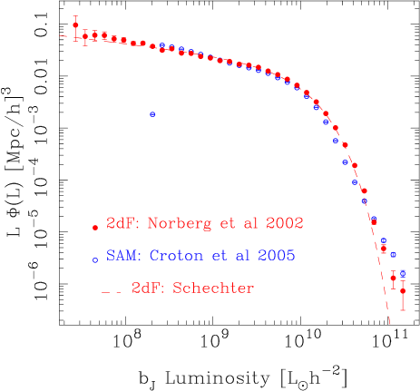
Figure 1, left panel, compares the 2dFGRS $b_{J}$ GLF with the GLF estimates obtained using Eq. (1) for the SAM galaxies. From this it can be seen that the Croton et al. (2006) galaxies do indeed provide a qualitatively good description of the 2dFGRS GLF. The largest deviations are noticeable for galaxies with $L>L_{\star}$. Also, we see the drop-off in the number density of objects present around $L\sim 2\times 10^{8}h^{-2}L_{\odot}$, due to the limited mass resolution of the simulation.

5.3 Conditional luminosity function

The CLF was first introduced by Yang et al. (2003). We now summarise their model, which has been highly successful at reproducing a large number of observational results from the 2dFGRS. Again, given a halo of mass $M$, the CLF returns the number of galaxies per unit luminosity interval ${\rm d}L$. It can be represented by a Schechter type function:

$$\Phi(L|M){\rm d}L=\tilde{\Phi}_{*}\left(\frac{L}{\tilde{L}_{*}}\right)^{\tilde{\alpha}}\exp\left[-\frac{L}{\tilde{L}_{*}}\right]\frac{{\rm d}L}{\tilde{L}_{*}}\ ,$$ (76)

where the three free parameters $\tilde{\Phi}_{*}\equiv\tilde{\Phi}_{*}(M)$, $\tilde{L}_{*}\equiv\tilde{L}_{*}(M)$ and $\tilde{\alpha}\equiv\tilde{\alpha}(M)$ are all mass dependent quantities. These parameters in turn are described by the following functions:

$$\tilde{\alpha} = \frac{}{}\alpha_{15}+\eta\log_{10}(M/[10^{15}h^{-1}M_{\odot}])\ ;$$ (77)

$$\tilde{L}_{*} = \frac{2M}{f(\tilde{\alpha})}\left[\left(\frac{M}{L}\right)_{0}\right]^{-1}\left[\left(\frac{M}{M_{1}}\right)^{-\beta}+\left(\frac{M}{M_{2}}\right)^{\gamma_{2}}\right]^{-1}\ ;$$ (78)

$$\tilde{\Phi}_{*} = \frac{\left<L\right>(M)}{\tilde{L}_{*}\Gamma[\tilde{\alpha}+1]}\ .$$ (79)

With the additional auxiliary functions:

$$\left<L\right>(M)=2M\left[\left(\frac{M}{L}\right)_{0}\right]^{-1}\left[\left(\frac{M}{M_{1}}\right)^{-\beta}+\left(\frac{M}{M_{1}}\right)^{\gamma_{1}}\right]^{-1}\ ;$$ (80)

$$f(\tilde{\alpha})=\frac{\Gamma[\tilde{\alpha}+2]}{\Gamma[\tilde{\alpha}+1,1]}\ ,$$ (81)

where $\Gamma[x]$ and $\Gamma[x,a]$ are the Gamma and incomplete Gamma functions, respectively:

$$\Gamma[x] = \int_{0}^{\infty}dzz^{x-1}\exp(-z)\ ;$$ (82)

$$\Gamma[x,a] = \int_{a}^{\infty}dzz^{x-1}\exp(-z)\ .$$ (83)

There are 8 free parameters in the above model, these are augmented by one final parameter $M_{\rm min}$, which specifies the minimum mass halo that may host a galaxy. For these 9 parameters we use the best-fit values reported in Yang et al. (2003): ${\bf p}=\{\alpha_{15}=-1.32,\ \eta=-0.36,\ \log_{10}M_{1}=10.42,\ \log_{10}M_{2}=11.74,\ (M/L)_{0}=102,\ \beta=0.6,\ \gamma_{1}=0.28,\ \gamma_{2}=0.69,\ \eta=-0.36,\ \log_{10}M_{\rm min}=9.0\}$.

Finally, the GLF can be obtained from the CLF, by integrating over the halo mass function as described in Eq. (19). Note, in evaluating Eq. (19), we follow exactly the recipe presented in Yang et al. (2003) and adopt the Sheth & Tormen (1999) mass function and the transfer function of Bardeen et al. (1986). This is necessary, since if we were to adopt other models, then we would expect the quoted parameters to no longer be the maximum likelihood parameter set. Since this is a first calculation we are not too worried by this, however for a more precise calculation one should reoptimise ${\bf p}$ for the true cosmological model.

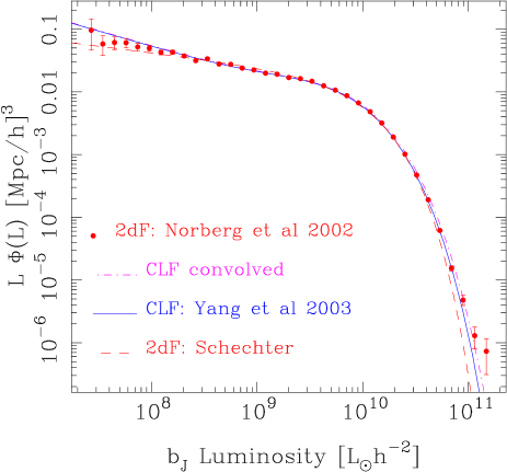
Figure 1, right panel, compares the 2dFGRS $b_{J}$ GLF with the GLF obtained from Eq. (19). As can be seen from the figure, the CLF model of Yang et al. (2003) (solid blue line) qualitatively provides a good description of the 2dFGRS data. Note, the optimised best-fit parameters described in the paper of Yang et al., do not take into account the presence of magnitude errors in the 2dFGRS data. If we convolve the model magnitudes with the log-normal distribution described in Norberg et al. (2002), then we find a small increase in the abundance of the brightest galaxies. Appendix B describes the inclusion of magnitude errors.

5.4 Luminosity dependence of galaxy clustering

In order to make predictions for the covariance matrix of the GLF we must also understand the luminosity dependence of the bias of the galaxy distribution. We explore this using the SAM galaxies (Croton et al., 2006). First, the galaxy catalogue is sliced into 8 bins in absolute magnitude. The exact magnitude bins that we employ and the numbers of galaxies in each bin are presented in Table 1. The correlation functions for the SAM galaxies were then estimated using our parallel tree-code correlation function algorithm DualTreeTwoPoint, which is based on the kD-Tree approach of Moore et al. (2001). The correlation functions were estimated in 40 logarithmically spaced bins in the radial interval $r\in[0.05,50.0]\,h^{-1}{\rm Mpc}$.

Figure 2: Correlation functions estimated from the Croton et al. (2006) semi-analytic galaxy catalogue in the Millennium simulation as a function of radial separation. The different coloured solid symbols show the results for the 8 absolute magnitude bins described in Table 1.

Figure 3: Relative scale dependence of galaxy bias measured for the different galaxy populations in the Millennium simulation semi-analytic galaxy catalogues of Croton et al. (2006). The relative bias is defined with respect to the lowest luminosity galaxy bin. The connected coloured points show the results for the 8 magnitude bins presented in Table 1.

Table 1: Table showing: Col. 1: bin number; Col 2: the absolute magnitude limits of the bin; Col. 3: Number of galaxies within the bin from which we calculate the correlation functions.

Bin	Magnitude range	Number of
Number	$[M_{b_{\rm J}}-5\log_{10}h]$	Galaxies
1	$[<-20.8]$	15,448
2	$[-20.0,-20.8]$	130,447
3	$[-19.3,-20.0]$	471,467
4	$[-18.6,-19.3]$	876,150
5	$[-17.8,-18.6]$	125,4400
6	$[-17.1,-17.8]$	1,690,406
7	$[-16.4,-17.1]$	2,367,636
8	$[-15.6,-16.4]$	3,119,262

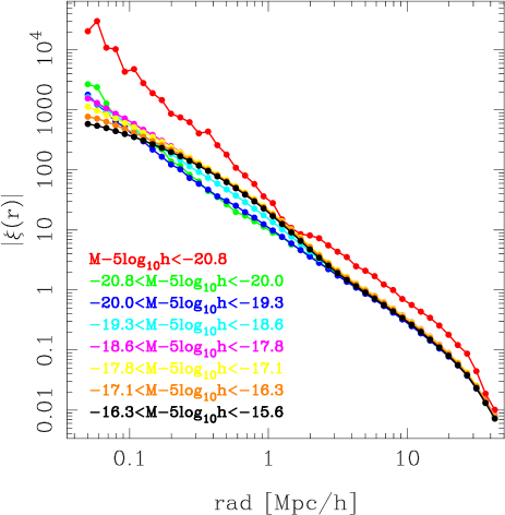
Figure 3 shows the results for the galaxy correlation functions measured in the 8 luminosity bins presented in Table 1. On scales $r>3\,h^{-1}{\rm Mpc}$ the signal appears to demonstrate a power-law like form and with the brightest sample of galaxies being significantly more correlated than the lower luminosity galaxies. On smaller scales, however the signal is more complex: there appears to be a strong scale-dependence with lower luminosity galaxies becoming more strongly correlated than intermediate luminosity galaxies.

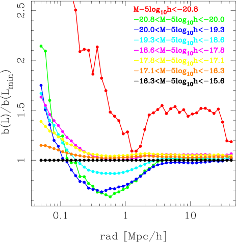
Figure 3 quantifies this scale-dependence in more detail, where we plot the relative bias of the SAM galaxies as a function of scale. We define the relative galaxy bias as:

$$b_{\rm rel}(L_{\mu},L_{\nu})\equiv\frac{b^{{\rm g}}(L_{\mu})}{b^{{\rm g}}(L_{\nu})}=\sqrt{\frac{\xi_{\rm gg}(r|L_{\mu})}{\xi_{\rm gg}(r|L_{\nu})}}\ .$$ (84)

The figure shows $b^{{\rm g}}_{\rm rel}(L_{\mu},L_{\rm min})$. On scales $r>3\,h^{-1}{\rm Mpc}$ the bias is reasonably flat for all of the bins, but that, interestingly, the lower luminosity galaxies can be more strongly correlated than the intermediate luminosity bins. Furthermore, it shows that on scales less than $r\sim 1\,h^{-1}{\rm Mpc}$ the brightest galaxy bins, with the exception of Bin 1, all possess a strong relative anti-bias, although Bin 1 does demonstrate a sharp dip at about the same scale. On still smaller scales, $r<100\,h^{-1}{\rm kpc}$, the relative bias becomes strongly positive. Owing to the fact that we are primarily interested in understanding the luminosity dependence of the large-scale bias, we shall reserve the understanding of this scale-dependence for future work.

We now focus on the large-scale relative bias. In most observational studies the relative bias is computed with respect to the characteristic luminosity $L_{*}$ of the survey. For the SAM galaxies, this approximately corresponds to the galaxies in Bin 3. For this work, our operational definition of ‘large scales’ is given by $\left(5\,h^{-1}{\rm Mpc}<r<30\,h^{-1}{\rm Mpc}\right)$.

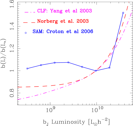
Figure 4 shows $b^{{\rm g}}_{\rm rel}(L_{\mu},L_{\nu}={\rm Bin\,3})$, and the luminosity dependence of the large-scale relative bias measured from the SAM galaxies is represented by the blue solid line. This may be compared with the results for the 2dFGRS obtained by Norberg et al. (2002):

$$\frac{b_{\rm 2dF}(L)}{b(L_{*})}=0.85+0.15\left(\frac{L}{L_{*}}\right)\ ,$$ (85)

and represented in the figure by the red-dashed line.

Interestingly, we see that the relative bias for the SAM galaxies is much flatter for faint objects than one finds for the 2dFGRS. The relative bias appears to have a minimum for $L_{*}$ galaxies and then increases slightly for fainter objects, whereas the bias steadily decreases for the 2dFGRS. However, the SAM galaxies do correctly capture the trend that the brightest galaxies in the 2dFGRS are more strongly correlated than the fainter ones. Thus, whilst the SAM galaxies are able to reproduce the GLF, they appear to only qualitatively capture the luminosity dependence of the clustering in the 2dFGRS. This failure of the Croton et al. (2006) model to correctly capture the luminosity dependence of the clustering has been noted in previous studies (Li et al., 2007; Kim et al., 2009; Guo et al., 2011). These have attributed the discrepancy between the observations and the model to the fact that, too many faint satellite galaxies are placed in the high mass haloes.

We may also obtain a prediction for the luminosity dependence of the bias using the CLF approach of Yang et al. (2003). On rewriting Eq. (33) in terms of the CLF we find,

$$b^{g}(L_{\mu})=\frac{1}{\phi(L_{\mu})}\int dM_{1}n(M_{1})b(M_{1})\Phi(L_{\mu}|M)\ .$$ (86)

We have evaluated the above integral using the model described in §5.3, and the results are represented by the dot-dashed line in Fig. 4. Clearly, this model appears to accurately reproduce the luminosity dependence of the clustering. However, this fact is not too remarkable, since the model was optimised using this data. The salient point is that we are able to reproduce the 2dFGRS results through evaluating Eq. (86).

Figure 4: Relative large-scale bias of galaxies as a function of luminosity. The dashed red line represents the results from the 2dFGRS presented in Norberg et al. (2002); the connected open blue points denote our estimates from the semi-analytic galaxy catalogues in the Millennium simulation (Croton et al., 2006); and the magenta dot-dashed line denotes the results from the conditional luminosity function model of Yang et al. (2003), which were constrained to match the 2dFGRS results.

6 Covariance of the galaxy luminosity function

In this section we test our theoretical model for the covariance matrix of the GLF estimates. We start with the volume limited sample, and then move on to the more complex scenario of the flux limited sample.

6.1 Results: Volume limited samples

We use the SAM galaxy catalogues to construct an estimate of the covariance matrix of the GLF in volume limited samples. We do this by following the approach for computing the cluster count covariance, which was described in Smith & Marian (2011). Briefly, we take the full volume of the Millennium simulation mock and slice it up into $n^{3}$ cubical cells. On taking $n=4$ we have 64 quasi-independent sub-volumes of size $L=125\,h^{-1}{\rm Mpc}$. For each of these sub-volumes we estimate the GLF in 27 equal logarithmically spaced luminosity bins using Eq. (1). From these 64 we construct the covariance matrix using the simple unbiased estimator:

$$\widehat{C}_{\mu\nu}=\frac{1}{n^{3}-1}\sum_{i=1}^{n^{3}}\left[\widehat{\phi}_{i}(L_{\mu})-\overline{\phi}(L_{\mu})\right]\left[\widehat{\phi}_{i}(L_{\nu})-\overline{\phi}(L_{\nu})\right]$$ (87)

where

$$\overline{\phi}(L_{\mu})=\frac{1}{n^{3}}\sum_{i=1}^{n^{3}}\widehat{\phi}_{i}(L_{\mu})\ .$$ (88)

We are interested in exploring errors for a survey with volume $V\sim 0.125\,h^{-3}\,{\rm Gpc}^{3}$, however, the above procedure provides us with the covariance matrix for survey volumes of the order $V=1.99^{-3}\,h^{-3}\,{\rm Gpc}^{3}$. We obviate this problem by approximating the covariance of the large volume to be the covariance on the mean, i.e.

$$\widehat{C}_{\mu\nu}(V)\approx\widehat{\overline{C}}_{\mu\nu}(V/n^{3})\equiv\widehat{C}_{\mu\nu}(V/n^{3})/n^{3}\ .$$ (89)

Furthermore, in order to make predictions from the theory we must compute $\sigma^{2}_{V}$, i.e. Eq. (29). This requires us to specify the survey window function. As described in Smith & Marian (2011), one must actually be quite careful when computing this: if one wants to compare predictions with results from simulations then one needs to use the exact density modes that are in the box; if one wants to make predictions for the real Universe then the simulations fail to capture this correctly when the box-length $L$ is comparable with the dimensions of the survey. In this case one should use theoretical predictions. Since here we are comparing with $N$-body simulations, a good approximation is to interpret the survey volume as being spherical in the following way:

$$R=\left(\frac{3{V_{\rm s}}}{4\pi}\right)^{1/3}$$ (90)

and take the window function to be

$$W(k|R)=\frac{3}{y^{3}}\left[\sin y-y\cos y\right]\ ;\ y\equiv kR\ .$$ (91)

Hence, the volume variance takes the simple form

$$\sigma^{2}_{V}=\int_{0}^{\infty}\frac{dkk^{2}}{2\pi^{2}}\left|W(k|R)\right|^{2}P(k)\ .$$ (92)

Figure 5: Fractional errors in the galaxy luminosity function for a volume limited survey as a function of galaxy luminosity. The circular open points represent estimates obtained from the SAM galaxies. The solid blue line presents the total prediction of the theoretical model given by Eq. (36). The red dashed line denotes the contribution to the error from the sample variance; the green dot-dashed line corresponds to the error coming from the halo occupancy covariance; the magenta dotted line corresponds to the error from Poisson noise.

6.1.1 Diagonal errors

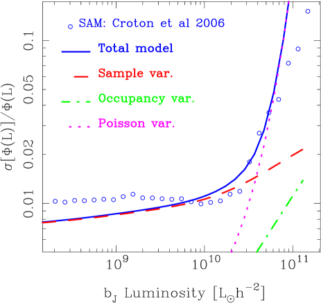
Figure 5 shows the diagonal elements of the covariance matrix divided by the ensemble average GLF estimates from the 64 sub-cubes in the Millennium simulation (open points) as a function of luminosity. In this figure, we also compare these results with the theoretical predictions from Eq. (36), where we have used the CLF model of Yang et al. (2003) as the model input. From Eq. (36) we find that,

$$\frac{\sigma^{2}[\phi(L_{\mu})]}{\phi^{2}(L_{\mu})}=[b^{\rm g}_{\mu}]^{2}\sigma^{2}_{V}+\frac{1}{N^{\rm g}_{\mu}}+\frac{\Sigma_{\mu\mu}}{\phi_{\mu}^{2}}\ .$$ (93)

The above expression informs us that: in the limit where the sample variance is dominant, which for this case occurs when $N^{\rm g}_{\mu}>10^{4}$, we have:

$$\left.\frac{\sigma[\phi(L_{\mu})]}{\phi(L_{\mu})}\right|_{\rm S.V.}=b^{\rm g}_{\mu}\sigma_{V}\ ;$$ (94)

and in the limit where the Poisson noise is dominant, which for this case occurs when $N^{\rm g}_{\mu}<10^{4}$, we have:

$$\left.\frac{\sigma[\phi(L_{\mu})]}{\phi(L_{\mu})}\right|_{\rm P.V.}=\frac{1}{\sqrt{N^{\rm g}_{\mu}}}\ .$$ (95)

The luminosity dependence of the halo occupancy variance scales as

$$\left.\frac{\sigma[\phi(L_{\mu})]}{\phi(L_{\mu})}\right|_{\rm O.V.}=\frac{\sqrt{\widetilde{\Sigma}_{\mu\mu}}}{\sqrt{N^{\rm g}_{\mu}}}$$ (96)

where $\widetilde{\Sigma}_{\mu\mu}$ is given by Eq. (49). We see from the denominator that this term scales in a similar way to the Poisson noise.

Figure 6: Relative importance of the halo occupancy variance $\widetilde{\Sigma}_{\mu\mu}$ (c.f. Eq. (49)) with respect to the Poisson errors, as a function of the luminosity bin. Poisson errors dominate as $\widetilde{\Sigma}_{\mu\mu}\ll 1$. Note that this is independent of survey volume.

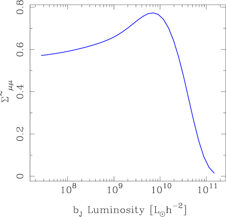
Figure 5 shows that the theory and the measurements from the SAM are in excellent agreement. Further the above limiting cases are clearly demonstrated by the data. Note that for low-luminosities the errors in the SAM data appear to be slightly in excess of the theoretical predictions. From Eq. (94) we see that this can be attributed to the fact that the luminosity dependence of the bias in the SAMs is in excess of the bias one obtains from the CLF approach (c.f. discussion surrounding Fig. 4).

The above results are for a particular choice of ${V_{\rm s}}$ and in principle, for a sufficiently large survey, ${V_{\rm s}}\sigma({V_{\rm s}})\rightarrow 0$, we are left with just the halo occupancy covariance and the Poisson noise. Figure 6 presents the ratio of the halo occupancy variance with respect to the Poisson noise, i.e. $\sigma^{2}[\phi(L_{\mu})]_{\rm O.V.}/\sigma^{2}[\phi(L_{\mu})]_{\rm P.V.}=\widetilde{\Sigma}_{\mu\mu}$. This demonstrates that for the brightest galaxies in a survey, the counts are dominated by Poisson errors. However, for the fainter galaxies $L\lesssim L_{*}$ the halo occupancy variance is roughly between $\sim 0.6$–$0.8$ times the Passion noise, independent of the survey volume. Note that this fractional relation between the halo occupancy variance and the Poisson errors holds exactly for both volume and flux-limited surveys.

6.1.2 Correlation matrix

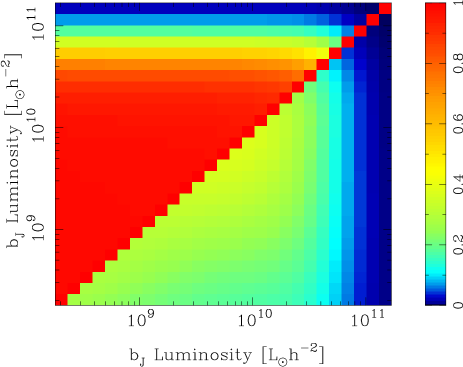
Figure 7 presents the relative contributions to the correlation matrix. The top left triangle shows the sample covariance plus Poisson noise correlation matrix, with the halo occupancy covariance set to zero. The bottom right triangle shows the halo occupancy covariance plus Poisson noise, with the sample variance set to zero. This demonstrates that, for the case of a volume limited 2dFGRS-like survey, with volume of size $V=0.125\,h^{-3}\,{\rm Gpc}^{3}$, the off-diagonal elements of the covariance matrix are entirely dominated by the sample variance term. However, following our earlier discussion from §4.3, we now point out that if our survey was sufficiently large, such that ${V_{\rm s}}\sigma({V_{\rm s}})\rightarrow 0$, then the matrix would still be correlated and that this would be given exactly by the bottom right panel of Fig. 7. The figure shows that the minimum correlation coefficient that could be obtained for galaxies with $L\lesssim L_{*}$ is roughly $r\sim 0.2$–$0.4$.

The left panel of Fig. 8 presents the correlation matrix constructed from the estimates of the covariance matrix obtained through application of Eq. (87) to the SAM data. The results show that the GLF estimates for galaxies with luminosities $L<L_{*}$ are almost perfectly correlated, i.e. $r\sim 1$. This is a somewhat startling result, as it means that if there is an upward fluctuation of one bin with respect to the mean then all other bins share that same upwards fluctuation. As we will discuss later, this has broad implications for how one fits models to the measured GLF data.

The right panel of Fig. 8, presents our theoretical predictions for the correlation matrix, evaluated using Eq. (41) and the CLF model of Yang et al. (2003). We find that the theoretical predictions are in remarkably good agreement with the estimates from the SAM. The theoretical predictions are slightly more correlated than the measurements from the SAM. This might be attributed to the mis-match in the luminosity dependence of the galaxy bias from the SAM and the 2dFGRS CLF model.

Figure 7: Relative contributions of the sample and halo occupancy covariance to the correlation matrix, for a volume limited sample of galaxies. The upper left triangle represents the sample variance plus Poisson noise contribution, with the halo occupancy covariance set to zero. The lower right triangle represents the halo occupancy covariance plus Passion noise contribution, with the sample variance set to zero.

   

Figure 8: Correlation matrix of luminosity function estimates for a volume limited sample of galaxies. Left panel: results obtained from the semi-analytic galaxies in the Millennium simulation. Right panel: results obtained from the theoretical model described in Eq. (41).

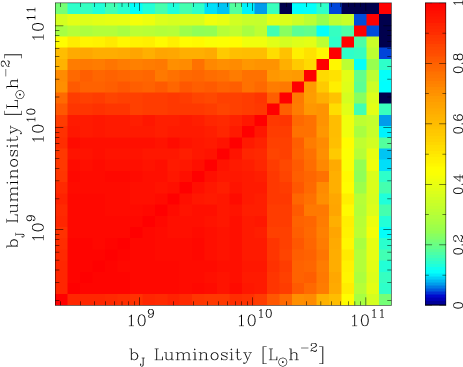
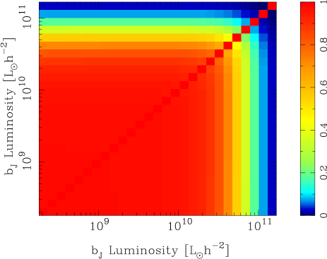
6.2 Results: Flux limited samples

Having validated our theoretical model for the covariance matrix of the GLF, we now turn to the slightly more complicated case of predicting the covariance matrix for a flux limited survey.

As described in §4 we must take into account that, for a flux-limited survey, the observed volume depends on the luminosity of the objects in question and the flux limit. We shall take our fiducial survey to have an angular area coverage of roughly $\Omega_{\rm s}\sim 1000\,{\rm deg^{2}}$. The survey volume will thus be $V_{\mu}^{\rm max}=\Omega_{\rm s}\chi^{\rm max}(L_{\mu})/3$, where $\chi^{\rm max}(L_{\mu})$ is given by Eq. (52). In order to make predictions we also need to know, $\sigma^{2}(L_{\mu},L_{\nu})$, and in order to avoid dealing with the real complex survey geometry, we shall make the approximation that the cone volume can be interpreted simply as full-sky survey with radial dimension $R^{\rm max}(L_{\mu})\equiv[V_{\mu}^{\rm max}]^{1/3}$. Hence we employ the window function appropriate for a spherical-top-hat transformed into Fourier space:

$$W(k|L_{\mu})=\frac{3}{y^{3}}\left[\sin y-y\cos y\right]\ ;\ y\equiv kR^{\rm max}(L_{\mu})\ .$$ (97)

Further, we shall take the flux limit to be that equivalent to the 2dFGRS: $b_{J}=19.5$. In evaluating Eq. (52) we require the conversion from $b_{J}$–luminosity to $b_{J}$–absolute magnitude, and we do that using:

$$M(L_{\mu})=M_{\odot,b_{J}}-\frac{5}{2}\log_{10}\left[\frac{L_{\mu}}{L_{\odot}}\right]\ ,$$ (98)

where we have adopted $M_{\odot,b_{J}}=5.3$. Thus for galaxies with the characteristic luminosity of the 2dFGRS, we have $L_{*}=9.64\times 10^{9}h^{-2}L_{\odot}$, which corresponds to $M_{b_{J}}^{*}-5\log_{10}h=-19.66$, and the maximum distance out to which they may be observed corresponds to $\chi_{\rm max}\approx 680\,h^{-1}{\rm Mpc}$, and with the volume being $V_{\mu}^{\rm max}\approx 0.13\,h^{-3}\,{\rm Gpc}^{3}$.

6.2.1 Diagonal errors

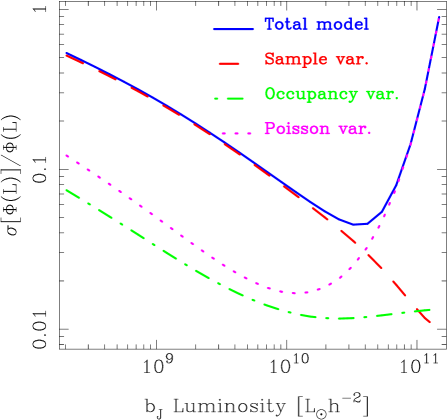
Figure 9 presents the predictions for the fractional errors on our fiducial survey. Considering again Eq. (69), we see that the fractional errors can be written:

$$\left.\frac{\sigma^{2}[\phi(L_{\mu})]}{\phi^{2}(L_{\mu})}\right|^{\rm FL}=[b^{\rm g}_{\mu}]^{2}\sigma^{2}(L_{\mu},L_{\mu})+\frac{1}{N^{\rm g}_{\mu}}+\frac{\Sigma^{\rm FL}_{\mu\mu}}{\phi_{\mu}^{2}}\ .$$ (99)

As for the case of the volume limited survey, the fractional errors have three contributions: the sample variance, the Poisson noise and the halo occupancy covariance. These three terms may also be described by Eqs (94)–(96).

In the figure we see that as in the case of the volume limited sample the fractional errors for the brightest galaxies are well described by the Poisson error term. However, for galaxies at the characteristic luminosity of the survey, the errors become dominated by the sample variance term. The interesting change from the volume limited survey is that when we consider the lower luminosity bins, we see that whilst the sample variance term is still dominant, the contributions from the Poisson variance and the halo occupancy variance are also significant. This owes to the fact that $V_{\mu}^{\rm max}$ is significantly smaller for galaxies with $L\sim L_{*}$ than for the case of the volume limited sample. Hence this leads to an increase in the Poisson shot noise for these bins. Finally, we recall that owing to the fact that $\widetilde{\Sigma}_{\mu\mu}^{\rm FL}=\widetilde{\Sigma}_{\mu\mu}$, the relative strength of the halo occupancy covariance to the Poisson noise is once more given by Fig. 6.

Figure 9: Fractional errors on the galaxy luminosity function for a survey of angular size $\Omega_{\rm s}\sim 1000\,{\rm deg}^{2}$, with limiting magnitude $b_{J}=19.5$ as a function of galaxy luminosity. The solid blue line presents the total prediction of the theoretical model given by Eq. (69). The red dashed line denotes the contribution to the error from the sample variance; the green dot-dashed line corresponds to the error coming from the halo occupancy covariance; the magenta dotted line corresponds to the error from Poisson noise.

Figure 10: Correlation matrix of luminosity function estimates for a survey of angular size $\Omega_{\rm s}\sim 1000\,{\rm deg}^{2}$ and with a flux limit $b_{J}=19.5$. Top panel: Relative contributions of the sample and halo occupancy covariance to the correlation matrix. The upper left triangle represents the sample variance plus Poisson noise contribution, with the halo occupancy set to zero. The lower right triangle shows the same for the halo occupancy plus Poisson noise covariance contribution, but this time with the sample variance set to zero. Bottom panel: total correlation matrix as given by Eq. (71).

6.2.2 Correlation matrix

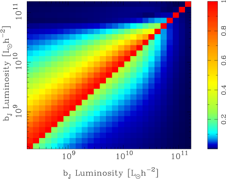
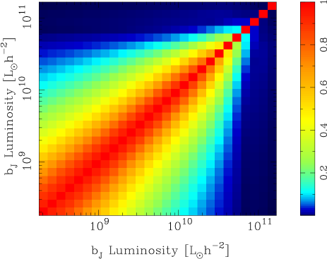
The top panel of Figure 10 presents the relative theoretical predictions for the correlation matrix. The top left triangle shows the contributions to the correlation matrix that come from the sample covariance plus Poisson noise, with the halo occupancy covariance set to zero. The lower right corner shows the same, but this time for the halo occupancy covariance plus Poisson noise, with the sample variance set to zero.

The bottom panel of Fig. 10 shows the theoretical predictions for the total correlation matrix of GLF estimates, as given by Eq. (71). We see that the correlation matrix is almost diagonal for galaxies with $L>6L_{*}$. However for galaxies with lower luminosities, the matrix becomes strongly correlated. The correlations are not as strong as for the Volume limited survey, however $r\sim 1$ for luminosity bins that are relatively close to one another.

Clearly, for our fiducial survey, the correlation matrix is dominated by the sample covariance, with a relatively small fraction of the off-diagonal elements coming from the occupancy covariance. However, for the case of a sufficiently large survey with $\sqrt{V_{\mu}^{\rm max}V_{\nu}^{\rm max}}\sigma^{2}(L_{\mu},L_{\nu})\rightarrow 0$, then the off-diagonal elements of the correlation matrix do not vanish, but are given by the bottom right triangle of Fig. 10 top panel.

7 Impact on Parameter estimation

We now explore the importance of including the covariance matrix when estimating GLF parameters from observations.

7.1 Methodology

Suppose we have estimated the GLF from our survey using either E1 or E2, depending on whether we have a flux or volume limited sample. We now wish to interpret these estimates in terms of some model. To do this, let us adopt the Bayesian framework. The probability of obtaining a data vector ${\bf x}$, given our model ${\mathcal{M}}$ with parameters ${\bm{\theta}}$, is described by the likelihood function ${\mathcal{L}}({\bf x}|{\bm{\theta}},{\mathcal{M}})$. A good choice for ${\mathcal{L}}$ is a multivariate Gaussian:

$${\mathcal{L}}({\bf x}|{\bm{\theta}},{\mathcal{M}})=\frac{1}{(2\pi)^{N/2}\sqrt{|{\rm\bf C}|}}\exp\left[-\frac{1}{2}({\bf x}-{\bm{\mu}})^{T}{\rm\bf C}^{-1}({\bf x}-{\bm{\mu}})\right]$$ (100)

where $\bm{\mu}\equiv\bm{\mu}(\bm{\theta})$ and ${{\rm\bf C}}\equiv{{\rm\bf C}}(\bm{\theta})$ are the model mean and model data covariance matrix, both of which depend on the parameters ${\bm{\theta}}$; and $|{\rm\bf C}|$ is the determinant of the matrix. Using Bayes theorem, the likelihood is directly related to the posterior probability distribution:

$$p(\bm{\theta}|{\bf x},{\mathcal{M}})=\frac{\Pi(\bm{\theta}|{\mathcal{M}}){\mathcal{L}}({\bf x}|\bm{\theta},{\mathcal{M}})}{p({\bf x}|{\mathcal{M}})}\ .$$ (101)

where $\Pi(\bm{\theta}|{\mathcal{M}})$ are a set of model priors, and $p({\bf x}|{\mathcal{M}})$ is termed the evidence, which simply can be written as a normalisation criterion: $p({\bf x}|{\mathcal{M}})=\int d{\bm{\theta}}\Pi({\bm{\theta}}|{\mathcal{M}}){\mathcal{L}}({\bf x}|{\bm{\theta}},{\mathcal{M}})$. The errors on the model parameters may be obtained through the exploration of the posterior distribution in the usual way (Press et al., 1992; Lewis & Bridle, 2002; Heavens, 2009). Different models ${\mathcal{M}}_{1}$ and ${\mathcal{M}}_{2}$ may then be compared using Bayesian model selection methods (Heavens, 2009).

If the priors $\Pi(\bm{\theta})$ are flat, then the posterior $p(\bm{\theta}|{\bf x})$ is simply proportional to the likelihood ${\mathcal{L}}$. Close to its maximum, at $\bm{\theta}_{0}$, we may Taylor expand the logarithm of the posterior, and for flat priors the log likelihood, to obtain:

$$\ln p(\bm{\theta}|{\bf x})\propto\ln{\mathcal{L}}({\bf x}|\bm{\theta}_{0})-\frac{1}{2}\sum_{\alpha,\beta}{\mathcal{H}}_{\alpha\beta}(\bm{\theta}_{0})\Delta\theta_{\alpha}\Delta\theta_{\beta}+\dots\ ,$$ (102)

where in the above $\Delta\theta_{\alpha}\equiv\left(\theta_{\alpha}-\theta_{\alpha,0}\right)$ are deviations of the parameters from the fiducial values, ${\mathcal{H}}_{\alpha\beta}\equiv-\partial^{2}\ln{\mathcal{L}}/\partial\theta_{\alpha}\partial\theta_{\beta}$ is the Hessian matrix, and the first derivative vanished at the maximum. We may rewrite the above expression for the posterior as,

$$p(\bm{\theta}|{\bf x})\approx\frac{\Pi(\bm{\theta})}{p({\bf x})}{\mathcal{L}}(\bm{\theta}_{0})\exp\!\left[-\frac{1}{2}\sum_{\alpha,\beta}\Delta\theta_{\alpha}{\mathcal{H}}_{\alpha\beta}(\bm{\theta}_{0})\Delta\theta_{\beta}\right]\ .$$ (103)

Thus ${\mathcal{H}}_{\alpha\beta}$ informs us about errors on the parameters and how different parameters may be correlated with respect to each other – in the context of their effects on the data.

For the case of a multivariate Gaussian posterior, the marginalised error on parameter $\theta_{\alpha}$, is given by $\hat{\sigma}^{2}_{\alpha\alpha}=1/\left[{\mathcal{H}}^{-1}\right]_{\alpha\alpha}$. Since the likelihood itself depends on the data, it is also a random variable. Taking an ensemble average over many realizations of the data, we arrive at the Fisher matrix:

$${\mathcal{F}}_{\alpha\beta}=\left<{\mathcal{H}}_{\alpha\beta}\right>=-\left<\frac{\partial^{2}\ln{\mathcal{L}}}{\partial\theta_{\alpha}\partial\theta_{\beta}}\right>\ .$$ (104)

From the Fisher matrix one may obtain the expected marginalised error on parameter $\theta_{\alpha}$ and the covariance between parameters $(\theta_{\alpha},\theta_{\beta})$:

$$\sigma_{\alpha\alpha}\geq\sqrt{\left[{\mathcal{F}}^{-1}\right]_{\alpha\alpha}}\ ;\hskip 28.45274pt\sigma_{\alpha\beta}\geq\sqrt{\left[{\mathcal{F}}^{-1}\right]_{\alpha\beta}}\ .$$ (105)

For a derivation of these error bounds see Heavens (2009).

Figure 11: Comparison of different Schechter function fits to semi-analytic model galaxy luminosity function data. The open points with errors denote the results from the Croton et al. (2006) model data. The red dot-dashed line and solid blue lines correspond to the best-fit Schechter functions obtained when fitting using only the diagonal elements of the data covariance matrix and when using the full data covariance matrix, respectively.

Under the assumption that the likelihood is Gaussian in the data, c.f. Eq. (100), then it can be shown that the Fisher matrix takes on the special form (Tegmark et al., 1997):

$${\mathcal{F}}_{\alpha\beta}=\frac{1}{2}{\rm Tr}\left[{\rm\bf C}^{-1}{\rm\bf C}_{,\alpha}{\rm\bf C}^{-1}{\rm\bf C}_{,\beta}\right]+{\bm{\mu}}_{\alpha}^{T}{\rm\bf C}^{-1}{\bm{\mu}}_{\beta}\ .$$ (106)

   

Figure 12: 2–D Likelihood contours for the luminosity function parameters $L_{*}$ and $\alpha$. Left panel: results obtained from a full exploration of the likelihood surface. The solid red ellipse and dashed red ellipse correspond to the 1– and 2–$\sigma$ confidence regions, respectively. These are obtained when we use only diagonal elements of the data covariance matrix in the parameter estimation. The solid blue ellipse and hatched blue ellipse, show the same, but when the full data covariance matrix is used. Right panel: Same as the left panel, except that the 1– and 2–$\sigma$ confidence regions are obtained using the Fisher matrix formalism, c.f. Eq. (110).

7.2 Best-fit Schechter function for SAM data

As a concrete example of our parameter estimation procedure, we now find the best-fit Schechter function parameters that describe the SAM data of Croton et al. (2006). We take the data for the volume limited sample of SAM galaxies described in §5.2. Again, we divide the full simulation volume into 64 equal sub-cubes and estimate the GLF for each using estimator E1. We then construct the mean GLF and its covariance matrix, as described in §6.1. We shall estimate the best-fit parameters for a survey region equivalent to a single sub-cube of size $L=125\,h^{-1}{\rm Mpc}$.

We adopt a Schechter function GLF model, as described by Eq. (75). As noted earlier, this has three parameters $\bm{\theta}=\{L_{*},\alpha,\phi_{*}\}$. We treat $L_{*}$ and $\alpha$ as free parameters and fix the normalisation $\phi_{*}$ by the constraint that we desire to recover the mean number density of galaxies in the volume that are above the luminosity cut $L_{\rm min}$:

$$\overline{n}_{\rm gal}=\int_{L_{\rm min}}^{\infty}dL\Phi(L|\bm{\theta})\ .$$ (107)

For the Schechter function this constraint is realised as:

$$\phi_{*}=\frac{\overline{n}_{\rm gal}}{\Gamma[\alpha+1,L_{\rm min}/L_{*}]}\ ,$$ (108)

where $\Gamma[x,a]$ is the incomplete Gamma function. We then construct the likelihood ${\mathcal{L}}$ as described by Eq. (100). This function is maximised with respect to the two free parameters, and we do this using an adaptive grid search scheme.

We find the 1– and 2–$\sigma$ confidence regions of the likelihood surface by identifying the contours in the ${\mathcal{L}}$–surface that satisfy:

$$p={\mathcal{L}}({\bf x}|\bm{\theta}_{0})\exp\left[-\Delta\chi^{2}/2\right]\ ,$$ (109)

where ${\mathcal{L}}({\bf x}|\bm{\theta}_{0})$ corresponds to the maximum of the likelihood and $\Delta\chi^{2}=\{2.3,6.17\}$ for 1– and 2–$\sigma$ contours, respectively.

The Fisher matrix approach of the previous section also provides us with a means for estimating the covariance matrix of parameters. From Eq. (106), and for a constant covariance matrix, the Fisher matrix for the GLF is:

$${\mathcal{F}}_{\alpha\beta}=\sum_{\mu,\nu}\frac{\partial\left[L\Phi(L_{\mu}|\bm{\theta})\right]}{\partial\theta_{\alpha}}{\rm\bf C}^{-1}_{\mu\nu}\frac{\partial\left[L\Phi(L_{\nu}|\bm{\theta})\right]}{\partial\theta_{\beta}}\ .$$ (110)

For the Schechter function parameters, the derivatives of interest are:

$$\frac{\partial\log\left[L\Phi(L|\bm{\theta})\right]}{\partial L_{*}} = \left[\frac{L-(\alpha+1)L_{*}}{L_{*}^{2}}\right]\ ;$$ (111)

$$\frac{\partial\log\left[L\Phi(L|\bm{\theta})\right]}{\partial\alpha} = \log\left[\frac{L}{L_{*}}\right]\ ;$$ (112)

$$\frac{\partial\log\left[L\Phi(L|\bm{\theta})\right]}{\partial\phi_{*}} = \frac{1}{\phi_{*}}\ .$$ (113)

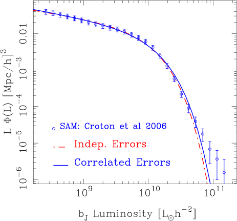
Figure 11 shows the best-fit Schechter function obtained when we fit the SAM GLF data using the full data covariance matrix (solid blue line), which correctly takes into account the effects of bin-to-bin correlations generated by the large-scale structure in the volume. The figure also shows the best-fit Schechter function model, obtained when we use only the diagonal elements of the data covariance matrix for the parameter estimation (red dot dashed line). It can be clearly seen that when we only use the diagonal elements of the covariance matrix, the model is biased. This owes to the fact that the fit gives more importance to the lower luminosity bins, for which the errors are significantly smaller than for the brighter bins. We may see this bias more clearly by exploring the likelihood surface directly.

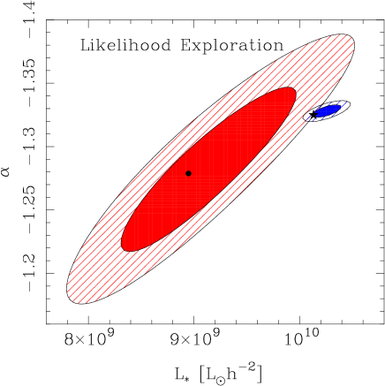
In the left panel of Figure 12 we show the 2-D likelihood surfaces for the fitted parameters $L_{*}$ and $\alpha$, and the 1– and 2–$\sigma$ confidence limits. The left panel shows the results obtained when we employ a full exploration of the likelihood surface. The blue ellipses show the results obtained when using the full data covariance, and the red ellipses show the results when using the diagonal elements of the covariance only. This figure shows the best-fit values for $\{L_{*},\alpha\}$ are only just consistent at the 2–$\sigma$ level. The best fit parameters are:

$$\bm{\theta}^{\rm full\,cov.}=\left\{\begin{array}[]{rl}L_{*}&=1.023\times 10^{10}\,[h^{-2}L_{\odot}]\\ \alpha&=1.325\\ \phi_{*}&=0.0122\ [h^{3}{\rm Mpc}^{-3}]\end{array}\right.\ .$$ (114)

$$\bm{\theta}^{\rm diag.\,cov.}=\left\{\begin{array}[]{rl}L_{*}&=8.913\times 10^{9}\,[h^{-2}L_{\odot}]\\ \alpha&=1.28\\ \phi_{*}&=0.0144\ [h^{3}{\rm Mpc}^{-3}]\end{array}\right.\ .$$ (115)

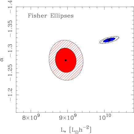
In the right panel of Figure 12 we show the results obtained when we employ the Fisher matrix formalism to calculate the parameter covariance matrix. Considering the case where we used the full data covariance matrix in the parameter estimation, we see that the Fisher matrix predictions are in excellent agreement with the full likelihood exploration. However, for the case where we used only the diagonal elements of the covariance matrix in the fitting, we find that the Fisher matrix errors are only qualitatively consistent with the results for the full likelihood exploration.

8 Conclusions

In this paper we have investigated the galaxy luminosity function (GLF) and what determines its error properties for various commonly used estimators.

In §2 we described several commonly used estimators for the GLF. We showed that Turner’s estimator (Turner, 1979), which attempts to correct for the effects of large-scale structure on the GLF, is actually a biased estimator.

In §3 we then focused on the simpler estimator of Schmidt (1968) for volume limited samples. Using a cluster expansion approach, we showed that this estimator in the ensemble limit was unbiased. We derived the covariance matrix of this estimator and found that it was comprised of three terms. The first term takes account of the sample variance, which depends on the biases of the galaxies in the different luminosity bins and also the variance of matter fluctuations in the survey volume. The second term was a simple Poisson noise contribution. The third term was dubbed halo occupancy covariance, and it arose due to the fact that several galaxies may be hosted by the same dark matter halo. We proved that the necessary requirement for sample covariance to vanish is: $\sigma^{2}{V_{\rm s}}\rightarrow 0$.

In §4 we investigated the $1/V^{\rm max}$ estimator of (Schmidt, 1968) for flux-limited surveys. We showed, in the ensemble limit, that this is also an unbiased estimator. We derived the covariance properties of the estimator. Similar to the case of the volume limited estimator, this matrix could also be decomposed into three terms: sample, Poisson and occupancy covariance terms. For the sample variance term, the major difference was that one must consider the cross-volume variance, since two distinct luminosity bins trace two different sample volumes. Again the necessary condition for the sample variance to be subdominant was attained when $\sigma^{2}[L_{\mu},L_{\mu}]V_{\mu}^{\rm max}\rightarrow 0$.

In §5 we described the semi-analytic model (SAM) galaxy catalogue of Croton et al. (2006) that we used to test our theoretical model. We also summarised the conditional luminosity function (CLF) model of Yang et al. (2003). We showed that for the volume limited estimator, both the SAM and CLF models were able to reproduce the 2dFGRS GLF. We then investigated the luminosity dependence of the galaxy bias, and showed that in the SAM model the correlation functions for different luminosity binned samples showed complicated scale-dependence. For $r>3\,h^{-1}{\rm Mpc}$ the bias was reasonably flat. We measured the large-scale relative bias and found that the brightest luminosity bin, $L>3\times 10^{10}h^{-2}L_{\odot}$, showed a 50% larger bias relative to $L_{*}$ galaxies. For galaxies with $L<L_{*}$ we found that the SAM model predicted a much flatter luminosity dependence of the bias than was measured in the 2dFGRS. The CLF model, by fiat, reproduced the 2dFGRS data. These results were in agreement with earlier work (Li et al., 2007; Kim et al., 2009; Guo et al., 2011).

In §6 we used the SAM galaxies to examine the fractional errors on the GLF estimates from the volume limited samples. We found that for the bright galaxies the fractional errors were much larger than for the fainter bins. For these, however the fractional error became flat below $L_{*}$. The errors were not reduced as the number of galaxies in the bin dramatically increased. These results were in excellent agreement with our predictions from the theoretical model. This plateau effect was explained by the sample variance being the dominant source of error for these luminosity bins.

Again using the SAM galaxies we estimated the covariance matrix of the estimates of the GLF. We found that for the Millennium simulation volume, the cross-correlation coefficient was $r<0.5$ only for galaxies with $L>5\times 10^{10}h^{-2}L_{\odot}$. For lower luminosity galaxies $r>0.5$ and at the faint end the matrix was almost perfectly correlated. We showed that the theoretical predictions from our theoretical model was again in excellent agreement.

We then used our theoretical model to make predictions for how the errors would change for a GLF estimated from a flux limited survey. For the fractional errors, the main differences from the volume limited sample, were that for the low luminosity bins the errors increased with decreasing luminosity. This owed to the reduced surveyed volume for these bins. However, the sample variance was still dominant on these scales. Exploring the covariance matrix, we found that in this case the matrix was less correlated than for the volume limited sample. However, the matrix was still highly correlated for the galaxies with $L<L_{*}$. Again the off-diagonal covariance was attributed to the sample variance term.

In §7 we explored the importance of including the full data covariance matrix when interpreting observations in terms of a given model. We showed that if one neglects the bin-to-bin covariances in the luminosity function, then parameter estimates will be biased. When fitting Schechter functions to data, we found that the most seriously affected was the characteristic luminosity, which was systematically under-estimated by 10-20%.

Appendix A Cluster count statistics

In this appendix we calculate $\left<N^{\rm c}_{\alpha}\right>_{P,s}$ and $\left<N^{\rm c}_{\alpha}N^{\rm c}_{\beta}\right>_{P,s}$. These derivations follow from Hu & Kravtsov (2003) and Smith & Marian (2011).

Consider some large cubical patch of the Universe, of volume ${V_{\rm s}}$, and containing $N$ clusters that possess some distribution of masses. Let us subdivide the cluster population into a set of $N_{m}$ mass bins. Let the number of clusters in the $\alpha^{\rm th}$ mass bin be denoted $N^{\rm c}_{\alpha}$. We shall assume that the probability that the volume contains $N^{\rm c}_{\alpha}$ clusters in the mass bin $\alpha$, is a Poisson process:

$$P(N^{\rm c}_{\alpha}|m_{\alpha})=\frac{m_{\alpha}^{N^{\rm c}_{\alpha}}\exp(-m_{\alpha})}{N^{\rm c}_{\alpha}!}\ .$$ (116)

For any quantity $X$ that depends on the number of clusters, we denote the average over the sampling distribution–the Poisson process in this case–as $\left<X\right>_{P}$. Thus, the average of $N^{\rm c}_{\alpha}$ over the sampling distribution can be written:

$$\left<N^{\rm c}_{\alpha}\right>_{P}=m_{\alpha}\equiv\overline{m}_{\alpha}\left[1+\overline{b}_{\alpha}{\delta}_{V}({\bf x})\right],$$ (117)

where $\overline{m}_{\alpha}=\overline{n}_{\alpha}V$ is the expected number of counts averaged over the Poisson sampling distribution and the density fluctuations ${\delta}_{V}({\bf x})$ in the volume. The volume of the survey and the volume-averaged overdensity field, are written:

$${V_{\rm s}} = \int{\rm d}^{3}{\!\bf x}^{\prime}\,W({\bf x}^{\prime}|{V_{\rm s}})\ \ ;$$ (118)

$${\delta}_{V}({\bf x}) = \frac{1}{{V_{\rm s}}}\int{\rm d}^{3}{\!\bf x}^{\prime}\,W({\bf x}^{\prime}|{V_{\rm s}})\delta({\bf x})\ .$$ (119)

where $W({\bf x}|{V_{\rm s}})$ is the window function for the survey and $\overline{n}_{\alpha}$ and $\overline{b}_{\alpha}$ are given by Eqs (16) and (28).

Following Lima & Hu (2004) we take the likelihood of drawing a particular set of cluster counts in the mass bins to be ${\bf N}\in\{N^{\rm c}_{1},\dots,N^{\rm c}_{N_{m}}\}$ in the cells to be:

$${\mathcal{L}}({\bf N}|\overline{\bf m},{\bf S})=\int d^{\mathcal{N}}\!m\left[\prod_{\alpha=1}^{N_{m}}P(N_{\alpha}|m_{\alpha})\right]G({\bf m}|\overline{\bf m},{\bf S})\$$ (120)

where $\overline{\bf m}\in\{\overline{m}_{1},\dots,\overline{m}_{N_{\alpha}}\}$ is a model for the counts in the cells, ${\mathcal{N}}=N_{m}$ and where it was assumed that the statistics of the volume-averaged density field are described by a multivariate Gaussian:

$$G({\bf m}|\overline{\bf m},{\bf S})\equiv\frac{(2\pi)^{-N/2}}{|S|^{1/2}}\exp\left[-\frac{1}{2}({\bf m}-\overline{\bf m})^{T}{\bf S}^{-1}({\bf m}-\overline{\bf m})\right]\ ,$$ (121)

where ${\bf S}$ is defined to be

$$S_{\alpha\beta}\equiv\left<\left(m_{\alpha}-\overline{m}_{\alpha}\right)\left(m_{\beta}-\overline{m}_{\beta}\right)\right>_{s}$$ (122)

Note, we refer to averages over the density field as sample averages and for a quantity $X$, they will be denoted $\left<X\right>_{s}$.

At this point we may be more precise about what we mean by ensemble and Poisson averages:

$$\left<X({\bf N})\right>_{P,s}\equiv\sum_{N^{\rm c}_{1}=0}^{\infty}\dots\sum_{N^{\rm c}_{N_{m}}=0}^{\infty}{\mathcal{L}}({\bf N}|\overline{\bf m},{\bf S})X({\bf N})\ .$$ (123)

Equation (120) can be simplified in two limits: If $S_{\alpha}\ll\overline{m}_{\alpha}$, then the likelihood is the product of Poisson processes; alternatively, in the limit of a large number of counts in each cell, then the Poisson process becomes close to Gaussian and the likelihood can be approximated as a Gaussian with shifted mean and augmented covariance matrix:

$${\mathcal{L}}({\bf N}|\overline{\bf m},{\bf S})\approx G({\bf N}|\overline{\bf m},{\bf C})\ \ ;\ \ {\bf C}=\overline{{\bf M}}+{\bf S}\ ,$$ (124)

where $\overline{\bf M}\rightarrow\overline{M}_{\alpha\beta}=\delta^{K}_{\alpha,\beta}\overline{m}_{\alpha}$. Note that in the above equation, the approximate sign is used since negative number counts are formally forbidden (for a more detailed discussion of this see Hu & Cohn, 2006).

The covariance of the counts can be written

$$\left<N^{\rm c}_{\alpha}N^{\rm c}_{\beta}\right>_{s,P}\!\!\! =\!\!\! \!\!\!\sum_{N^{\rm c}_{1}=0}^{\infty}\dots\!\!\!\sum_{N^{\rm c}_{N_{m}}=0}^{\infty}\!\!\!{\mathcal{L}}({\bf N}|\overline{\bf m},{\bf S})N^{\rm c}_{\alpha}N^{\rm c}_{\beta}$$ (125)

$$= \int d^{{\mathcal{N}}}\!mG({\bf m}|\overline{\bf m},{\bf S})$$

$$\times \left[m_{\alpha}m_{\beta}\tilde{\epsilon}_{\alpha\beta}+\left<\left(N^{\rm c}_{\alpha}\right)^{2}\right>_{P}\delta^{k}_{\alpha\beta}\right]\ .$$

where $\tilde{\epsilon}_{\alpha\beta}=1$ when $\alpha\neq\beta$ and 0 otherwise. Considering the second term on the right-hand-side of the above equation, and recall that for the Poisson distribution we have: $\left<X^{2}\right>=\left<X\right>[1+\left<X\right>]$. Hence, on using this fact, and coupled with $\overline{m}_{\alpha}=\overline{n}(M_{\alpha})\Delta M_{\alpha}V$ we find:

$$\left<N^{\rm c}_{\alpha}N^{\rm c}_{\beta}\right>_{s,P}\!\!\! = \!\!\!\int d^{{\mathcal{N}}}\!mG({\bf m}|\overline{\bf m},{\bf S})\left[m_{\alpha}m_{\beta}+m_{\alpha}\delta^{K}_{\alpha,\beta}\right]$$ (126)

$$= \left[S_{\alpha\beta}+\overline{m}_{\alpha}\overline{m}_{\beta}+\overline{m}_{\alpha}\delta^{K}_{\alpha,\beta}\right]\ .$$

Appendix B Incorporating magnitude errors

The above analysis has so far included errors induced in the GLF that arise from large-scale structures and also the occupancy of galaxies in haloes. We now examine how the above results are modified in the presence of calibration errors in the magnitudes of the galaxies. Again, we shall look to the results from the 2dFGRS for illustration.

We take account of the mapping between the true luminosity $L$ and the observed $L^{{\rm o}}$ in the following way: the observed GLF can be written

$$\phi(L^{{\rm o}}_{\mu})=\int_{L^{{\rm o}}_{\mu}}^{L_{\mu+1}^{{\rm o}}}{\rm d}L^{{\rm o}}\int_{0}^{\infty}{\rm d}Lp(L^{{\rm o}}|L)\phi(L)\ ,$$ (127)

where galaxies are observed with luminosities in the bin $L^{{\rm o}}_{\mu}<L^{{\rm o}}\leq L^{{\rm o}}_{\mu+1}$. In the above the key new ingredient is the probability distribution for obtaining a luminosity $L^{{\rm o}}$ given the underlying true luminosity $L$. In Norberg et al. (2002), the observed $b_{J}$-band magnitudes, $m^{{\rm o}}$, of the 2dFGRS galaxies were found to have a calibration error that was well described by a Gaussian with width $\sigma_{m}=0.15$, with underlying true mean magnitude $m$. Hence,

$$p(L^{{\rm o}}|L) = p_{\rm G}(m^{{\rm o}}|m)\left|\frac{dm^{{\rm o}}}{{\rm d}L^{{\rm o}}}\right|$$ (128)

$$=\frac{1}{\sqrt{2\pi}\sigma_{M}}\exp\left[-\frac{(m-m^{{\rm o}})^{2}}{2\sigma_{M}^{2}}\right]\left|\frac{dm^{{\rm o}}}{{\rm d}L^{{\rm o}}}\right|$$

$$=-\frac{2L^{{\rm o}}\log_{e}10}{5\sqrt{2\pi}\sigma_{m}}\exp\left[-\frac{25\left(\log_{10}L/L^{{\rm o}}\right)^{2}}{8\sigma_{M}^{2}}\right]\ ,$$

where in the above equations we used the relation $L/L^{{\rm o}}=10^{-2/5(m-m^{{\rm o}})}$, to compute the Jacobean of the coordinate transformation: $|{\rm d}L^{{\rm o}}/dm^{{\rm o}}|=-2L^{{\rm o}}\log_{e}10/5$.

Thus, with magnitude error uncertainties included, the covariance matrix becomes,

$${\mathcal{C}}[L^{{\rm o}}_{\mu},L^{{\rm o}}_{\nu}] = \int_{L^{{\rm o}}_{\mu}}^{L_{\mu}^{{\rm o}}+1}{\rm d}L_{1}^{{\rm o}}\int_{L^{{\rm o}}_{\nu}}^{L_{\nu+1}^{{\rm o}}}{\rm d}L_{2}^{{\rm o}}$$ (129)

$$\times\int{\rm d}L_{1}p(L_{1}^{{\rm o}}|L_{1})\int{\rm d}L_{2}p(L_{2}^{{\rm o}}|L_{2})\,{\mathcal{C}}[L_{1},L_{2}]$$

On inserting Eq. (36) for the true covariance, the observed covariance can be written

$${\mathcal{C}}[L_{\mu}^{{\rm o}},L_{\nu}^{{\rm o}}]=\widetilde{\phi b^{g}}(L^{{\rm o}}_{\mu})\widetilde{\phi b^{g}}(L^{{\rm o}}_{\nu})\sigma^{2}({V_{\rm s}})+\frac{\widetilde{\phi}(L^{{\rm o}}_{\mu})\delta^{K}_{\mu,\nu}}{{V_{\rm s}}\Delta L^{{\rm o}}_{\mu}}$$

$$+\frac{1}{{V_{\rm s}}}\int dM_{1}n(M_{1})\widetilde{\phi}(L^{{\rm o}}_{\mu}|M_{1})\widetilde{\phi}(L^{{\rm o}}_{\nu}|M_{1})\ .$$ (130)

where we have defined three new terms:

$$\!\!\widetilde{\phi}(L^{{\rm o}}_{\mu}) \!\!\equiv \!\!\!\int_{L^{{\rm o}}_{\mu}}^{L_{\mu+1}^{{\rm o}}}\frac{{\rm d}L_{1}^{{\rm o}}}{\Delta L_{\mu}}\int_{0}^{\infty}{\rm d}L_{1}p(L_{1}^{{\rm o}}|L_{1})\phi(L_{1})\ ;$$ (131)

$$\!\!\widetilde{\phi b^{g}}(L^{{\rm o}}_{\mu}) \!\!\equiv \!\!\!\int_{L^{{\rm o}}_{\mu}}^{L_{\mu+1}^{{\rm o}}}\!\frac{{\rm d}L_{1}^{{\rm o}}}{\Delta L_{\mu}}\int_{0}^{\infty}\!{\rm d}L_{1}p(L_{1}^{{\rm o}}|L_{1})\phi(L_{1})b^{g}(L_{1})\ ;$$ (132)

$$\!\!\widetilde{\phi}(L^{{\rm o}}_{\mu}|M) \!\!\equiv \!\!\!\int_{L^{{\rm o}}_{\mu}}^{L_{\mu+1}^{{\rm o}}}\frac{{\rm d}L_{1}^{{\rm o}}}{\Delta L_{\mu}}\int_{0}^{\infty}{\rm d}L_{1}p(L_{1}^{{\rm o}}|L_{1})\phi(L_{1}|M)\ .$$ (133)

In the limit where the luminosity bins are sufficiently narrow that the integrand does not vary across the bin, then the first integral in the above equations may be approximated by the central value of the integrand, in accordance with the mean value theorem. Furthermore, since we take the error in the magnitude distribution to be a Gaussian of width $\sigma_{m}$, the limits of the second integral can be restricted to be $L_{\rm max}(L^{{\rm o}})$ and $L_{\rm min}(L^{{\rm o}})$. Hence

$$\!\!\widetilde{\phi}(L^{{\rm o}}_{\mu}) \!\!\approx \!\!\!\int_{L_{\rm min}(L^{{\rm o}})}^{L_{\rm max}(L^{{\rm o}})}{\rm d}L_{1}p(L_{1}^{{\rm o}}|L_{1})\phi(L_{1})\ ;$$ (134)

$$\!\!\widetilde{\phi b^{g}}(L^{{\rm o}}_{\mu}) \!\!\approx \!\!\!\int_{L_{\rm min}(L^{{\rm o}})}^{L_{\rm max}(L^{{\rm o}})}\!{\rm d}L_{1}p(L_{1}^{{\rm o}}|L_{1})\phi(L_{1})b^{g}(L_{1})\ ;$$ (135)

$$\!\!\widetilde{\phi}(L^{{\rm o}}_{\mu}|M) \!\!\approx \!\!\!\int_{L_{\rm min}(L^{{\rm o}})}^{L_{\rm max}(L^{{\rm o}})}{\rm d}L_{1}p(L_{1}^{{\rm o}}|L_{1})\phi(L_{1}|M)\ .$$ (136)

In practice, the upper and lower bounds on the integrals are computed by allowing the minimum ‘true’ magnitude, which contributes to an observed magnitude bin, to be 4$\sigma$ away from the mean, respectively. This gives,

$$L_{\rm max}/L^{{\rm o}} = 10^{-2/5(m^{\rm min}-m^{{\rm o}})}=10^{8/5\sigma_{m}}$$ (137)

$$L_{\rm min}/L^{{\rm o}} = 10^{-2/5(m^{\rm max}-m^{{\rm o}})}=10^{-8/5\sigma_{m}}\ .$$ (138)

On adopting the appropriate value for the 2dFGRS, $\sigma_{m}=0.15$, this leads us to adopt the integral limits $L_{\rm max}=1.74L^{{\rm o}}$ and $L_{\rm min}=0.575L^{{\rm o}}$.

References

- Bardeen et al. (1986) Bardeen J. M., Bond J. R., Kaiser N., Szalay A. S., 1986, ApJ, 304, 15
- Beijersbergen et al. (2002) Beijersbergen M., Hoekstra H., van Dokkum P. G., van der Hulst T., 2002, MNRAS, 329, 385
- Benson et al. (2003) Benson A. J., Bower R. G., Frenk C. S., Lacey C. G., Baugh C. M., Cole S., 2003, ApJ, 599, 38
- Binggeli et al. (1988) Binggeli B., Sandage A., Tammann G. A., 1988, Anual Reviews of Astronomy and Astrophysics, 26, 509
- Blanton et al. (2001) Blanton M. R., The SDSS Team 2001, Astronomical Journal, 121, 2358
- Blanton et al. (2003) Blanton M. R., The SDSS Team 2003, ApJ, 592, 819
- Bower et al. (2010) Bower R. G., Vernon I., Goldstein M., Benson A. J., Lacey C. G., Baugh C. M., Cole S., Frenk C. S., 2010, MNRAS, 407, 2017
- Cole et al. (2001) Cole S., The 2dFGRS Team 2001, MNRAS, 326, 255
- Cole (2011) Cole S., 2011, MNRAS, 416, 739
- Cole et al. (2000) Cole S., Lacey C. G., Baugh C. M., Frenk C. S., 2000, MNRAS, 319, 168
- Cooray (2006) Cooray A., 2006, MNRAS, 365, 842
- Croton et al. (2005) Croton D. J., The 2dFGRS Team 2005, MNRAS, 356, 1155
- Croton et al. (2006) Croton D. J., Springel V., White S. D. M., De Lucia G., Frenk C. S., Gao L., Jenkins A., Kauffmann G., Navarro J. F., Yoshida N., 2006, MNRAS, 365, 11
- Efstathiou et al. (1988) Efstathiou G., Ellis R. S., Peterson B. A., 1988, MNRAS, 232, 431
- Faber et al. (2007) Faber S. M., The DEEP2 and COMBO-17 Teams 2007, ApJ, 665, 265
- Felten (1976) Felten J. E., 1976, ApJ, 207, 700
- Folkes et al. (1999) Folkes S., The 2dFGRS Team 1999, MNRAS, 308, 459
- Guo et al. (2011) Guo Q., White S., Boylan-Kolchin M., De Lucia G., Kauffmann G., Lemson G., Li C., Springel V., Weinmann S., 2011, MNRAS, 413, 101
- Heavens (2009) Heavens A., 2009, ArXiv e-prints
- Hu & Cohn (2006) Hu W., Cohn J. D., 2006, PRD, 73, 067301
- Hu & Kravtsov (2003) Hu W., Kravtsov A. V., 2003, ApJ, 584, 702
- Hubble (1936) Hubble E., 1936, ApJ, 84, 158
- Ilbert et al. (2005) Ilbert O., The VVDS Team 2005, A&A, 439, 863
- Kauffmann & Charlot (1998) Kauffmann G., Charlot S., 1998, MNRAS, 297, L23+
- Kauffmann et al. (1999) Kauffmann G., Colberg J. M., Diaferio A., White S. D. M., 1999, MNRAS, 303, 188
- Kim et al. (2009) Kim H.-S., Baugh C. M., Cole S., Frenk C. S., Benson A. J., 2009, MNRAS, 400, 1527
- Kirshner et al. (1979) Kirshner R. P., Oemler Jr. A., Schechter P. L., 1979, Astronomical Journal, 84, 951
- Lewis & Bridle (2002) Lewis A., Bridle S., 2002, Phys. Rev., D66, 103511
- Li et al. (2007) Li C., Jing Y. P., Kauffmann G., Börner G., Kang X., Wang L., 2007, MNRAS, 376, 984
- Lima & Hu (2004) Lima M., Hu W., 2004, PRD, 70, 043504
- Loveday et al. (2012) Loveday J., Norberg P., Baldry I. K., Driver S. P., Hopkins A. M., Peacock J. A., The GAMMA Team 2012, MNRAS, 420, 1239
- Moore et al. (2001) Moore A. W., Connolly A. J., Genovese C., Gray A., Grone L., Kanidoris II N., Nichol R. C., Schneider J., Szalay A. S., Szapudi I., Wasserman L., 2001, in A. J. Banday, S. Zaroubi, & M. Bartelmann ed., Mining the Sky Fast Algorithms and Efficient Statistics: N-Point Correlation Functions. p. 71
- Norberg et al. (2002) Norberg P., Baugh C. M., Hawkins E., Maddox S., Madgwick D., Lahav O., Cole S., Frenk C. S., The 2dFGRS Team 2002, MNRAS, 332, 827
- Norberg et al. (2002) Norberg P., Cole S., Baugh C. M., Frenk C. S., The 2dFRGRS Team 2002, MNRAS, 336, 907
- Peebles (1980) Peebles P. J. E., 1980, The large-scale structure of the universe. Research supported by the National Science Foundation. Princeton, N.J., Princeton University Press, 1980. 435 p.
- Press et al. (1992) Press W. H., Teukolsky S. A., Vetterling W. T., Flannery B. P., 1992, Numerical recipes in FORTRAN. The art of scientific computing. Cambridge: University Press, —c1992, 2nd ed.
- Robertson (2010) Robertson B. E., 2010, ApJ, 713, 1266
- Sandage et al. (1979) Sandage A., Tammann G. A., Yahil A., 1979, ApJ, 232, 352
- Schmidt (1968) Schmidt M., 1968, ApJ, 151, 393
- Sheth & Tormen (1999) Sheth R. K., Tormen G., 1999, MNRAS, 308, 119
- Smith & Marian (2011) Smith R. E., Marian L., 2011, MNRAS, pp 1484–+
- Springel et al. (2005) Springel V., White S. D. M., Jenkins A., Frenk C. S., Yoshida N., Gao L., Navarro J., Thacker R., Croton D., Helly J., Peacock J. A., Cole S., Thomas P., Couchman H., Evrard A., Colberg J., Pearce F., 2005, Nature, 435, 629
- Strauss & Willick (1995) Strauss M. A., Willick J. A., 1995, Phys. Rep. , 261, 271
- Tegmark et al. (1997) Tegmark M., Taylor A. N., Heavens A. F., 1997, ApJ, 480, 22
- Trenti & Stiavelli (2008) Trenti M., Stiavelli M., 2008, ApJ, 676, 767
- Turner (1979) Turner E. L., 1979, ApJ, 231, 645
- Willmer et al. (2006) Willmer C. N. A., The DEEP2 Team 2006, ApJ, 647, 853
- Yang et al. (2003) Yang X., Mo H. J., van den Bosch F. C., 2003, MNRAS, 339, 1057
- Zucca et al. (2009) Zucca E., The zCOSMOS Team 2009, A&A, 508, 1217