A comparison of the galaxy peculiar velocity field with the PSCz gravity field– A Bayesian hyper-parameter method
Abstract
We constructed a Bayesian hyper-parameter statistical method to quantify the difference between predicted velocities derived from the observed galaxy distribution in the IRAS-PSC redshift survey and peculiar velocities measured using different distance indicators. In our analysis we find that the model–data comparison becomes unreliable beyond because of the inadequate sampling by IRAS survey of prominent, distant superclusters, like the Shapley Concentration. On the other hand, the analysis of the velocity residuals show that the PSC gravity field provides an adequate model to the local, , peculiar velocity field. The hyper-parameter combination of ENEAR, SN, A1SN and SFI++ catalogues in the Bayesian framework constrains the amplitude of the linear flow to be . For an rms density fluctuations in the PSC galaxy number density , we obtain an estimate of the growth rate of density fluctuations , which is in excellent agreement with independent estimates based on different techniques.
Key words: methods: data analysis – methods: statistical – Galaxies: kinematic and dynamics – Cosmology: observations – large-scale structure of Universe
1 Introduction
The study of peculiar velocity is a powerful tool to explore the large-scale structure of the Universe. In the standard CDM cosmology, gravitational instability causes the growth of density perturbations and the emergence of the peculiar velocity field. In the regime where the density perturbation is linear, the galaxy peculiar velocity (), sourced by the underlying density field, can be expressed as (, 1993)
| (1) |
where is the Hubble parameter at the present epoch, is the present day growth rate (henceforth we drop the subscript ) and is the perturbation to the underlying dark matter distribution, i.e. . Assuming that the observable galaxy distribution links to the underlying dark matter distribution through a linear, deterministic bias factor, , one can express the above equation by substituting the growth rate of density fluctuations with the dimensionless parameter . According to Eq. (1) the amplitude of the velocity field scales linearly with and this parameter fully characterises the model velocity field (, 1993). The value of can be estimated by comparing the model velocities predicted from Eq. (1) to measured peculiar velocities estimated from distance indicators. A good match between these two vector fields would then constitute an observational test for the gravitational instability paradigm and for the CDM model (, 2001, 2001, 2002). Performing such a test is the aim of this paper.
Comparisons of – require all-sky redshift surveys to sample the mass distribution in the local Universe in a dense and homogeneous way. For this reason, a large number of studies have used the IRAS 1.2 Jy and PSC (Point Source Catalogue) redshift catalogues (, 1995, 2000). The latter, which we shall use in this work, covers about per cent of the sky, contains 12,275 galaxies at a mean distance of , and still represents the densest redshift catalogue available to date. Indeed, the recent 2MRS (Two Micron All Sky Redshift Survey) catalogue (, 2012) has a larger depth and better completeness than PSC, but its sampling within is sparser.
IRAS redshift catalogues have been extensively used to perform – comparisons to estimate . (1996) compared the gravity field obtained from the 1.2 Jy IRAS redshift survey with the Tully-Fisher (TF) peculiar velocities of spiral galaxies in the composite Mark III catalogue. The presence of systematic discrepancies between the two fields precluded the possibility of measuring . The likelihood technique developed by (1997, 1998) was designed to calibrate separately the different subsamples that constitute the Mark III catalogue. This allowed these authors to eliminate these discrepancies and to estimate from 838 galaxies with TF distances. An independent comparison performed by (1998) using peculiar velocities measured from the -band TF survey of field spirals (SFI, 1997, 1999) found . The same likelihood approach as (1997) was used by (2001) to compare SFI galaxies having TF-peculiar velocities with the PSC model velocity field. They found that the a linear field with provides a good match to observations. (2002) applied a different technique to estimate a continuous velocity field from the measured velocities of both early and late type galaxies in the ENEAR (, 2000; Bernardi et al., 2002; , 2003) and SFI catalogues. They showed that the PSC gravity field matches well this velocity field for .
Not all – comparisons use TF peculiar velocities. (2001) compared PSC with the ENEAR early-type galaxies having – velocities and found . (2004) and (2012) considered peculiar velocities of Type Ia supernovae. They considered two different compilations of objects and found and , respectively. More recently, 2MASS (Two Micron All Sky Survey) galaxies (Skrutskie et al., 2006) were also used to perform – comparison. (2005) compared the gravity field predicted from 2MASS photometry and public redshifts to different peculiar velocity surveys and found . Finally, (2011) compared the flow traced by the SFI++ sample of TF velocities (, 2006, 2007) to that predicted by the 2MRS sample of galaxies brighter than and found a best fit value .
All these studies assume that is independent of scale. Since in the standard gravitational instability framework is a scale-independent quantity, this assumption implies that galaxy bias is deterministic and linear. In fact, physical processes related to galaxy formation and evolution result in a scale-dependent and stochastic bias on small scales, but have little impact on – analyses in which the distribution of mass tracers is smoothed out on larger scales.
The scatter among values obtained from different – comparisons comes from several sources such as: (i) the use of different techniques to predict the gravity field and compare it with measured velocities; (ii) inadequate modelling of the flow in high density environment; (iii) the use of different mass tracers to model peculiar velocities; (iv) the use of different velocity tracers that preferentially sample different environments; (v) the possible systematic errors in the calibration of the distance indicator; (vi) possible systematic errors in the use of the distance indicators like the Malmquist bias (, 1920, 1988, 1994, 1995); and (vii) systematic biases in the model gravity field, e.g. the so-called ‘Kaiser rocket effect’ (, 1989, 2011, 2012).
These considerations together with the improved quality of the peculiar velocity data, better understanding of the systematics and advances in the modelling techniques, lead us to re-examine the issue. In this paper we make an extensive comparison between peculiar velocity data from different distance indicators and the PSC density field (, 1999). The rationale behind using different peculiar velocity catalogues is manifold. First, by performing independent – comparisons we can identify and correct for systematic errors in the measured velocities. Second, peculiar velocities from different distance indicators have different random errors and therefore require different Malmquist bias corrections. Third, possible additional sources of systematics can be identified by analyzing the residuals in the – comparisons restricted to the individual catalogues. Finally, we aim at estimating by performing a joint comparison that involves different velocity catalogues. For this purpose we will use a Bayesian ‘hyper-parameter’ method (, 2000, 2002) designed for this purpose.
This paper is organized as follows. In Section 2 we present the PSC galaxy catalogue and the model velocity field observations. In Section 3 we describe the four peculiar velocity catalogues considered in this work and the strategy we adopt to correct for Malmquist bias. The Bayesian approach adopted to perform the – comparison is introduced in Section 4 and the results, including the estimate of are presented in Section 5. Finally, in Section 6, we discuss our main conclusions.
2 Model peculiar velocities
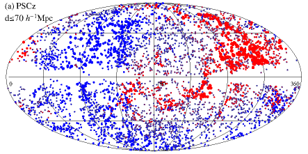
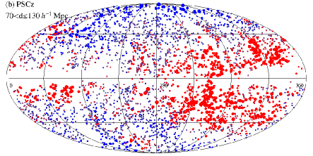
The first ingredient of the – comparison is the model velocity field. In this work we adopt the one obtained (, 1999) from the IRAS PSC catalogue (, 2000). Panels (a) and (b) of Fig. 1 show the angular distribution of PSC galaxies in Galactic coordinates. Panel (a) shows objects within a predicted distance of . This is the distance within which we shall perform – comparisons. Panel (b) shows objects in the shell covering –.
Objects in the PSC redshift catalogues were used to trace the underlying mass density field within under the assumption of linear and deterministic bias (, 2004). The model velocity field was obtained from the positions of galaxies in redshift space according to Eq. (1), using the iterative technique of (1991). Iterations involve only objects within . At larger distances the sampling becomes very sparse and objects are used to model an external gravity field, but their peculiar velocities are not used directly.
The iterative procedure is potentially prone to systematic errors. Here is a short description of the main ones and how to fix them:
-
1.
Incomplete sky coverage. The surface density of observed galaxies drops abruptly near the Galactic Plane, in the so-called Zone of Avoidance (hereafter ZoA), clearly seen in panels (a) and (b) of Fig. 1. Different techniques have been proposed to fill this region and their impact on the final predictions is not large. (1994) and (2004) estimated that typical induced errors on are well below per cent, an upper limit obtained by filling the ZoA with a homogeneous distribution of fictitious galaxies. Here we use the filling method of (1999) that consists of randomly cloning the observed galaxy distribution from the nearby areas into the ZoA. The results obtained with this method were almost identical to those obtained using a Fourier-based technique (, 1999) and consistent with those of the Wiener-like filtering analysis of (2002). Analyses performed using mock PSC galaxy catalogues showed that the filling method used in this work induces a spurious bulk flow of but has negligible impact on the estimated (, 1999).
-
2.
Uncertainties in modelling the mass distribution beyond . These uncertainties mainly induce a dipole-like external field that we remove by computing peculiar velocities relative to the central observer (i.e. in the Local Group frame) and by restricting quantitative analyses to objects within .
-
3.
Treatment of high density regions. IRAS galaxies are preferentially late type and therefore undersample the cores of galaxy clusters. In addition, regions around high density peaks are ‘tripled valued’, i.e. the same redshift is observed at three different positions along the line of sight to the peak. To correct these effects we assign an appropriate statistical weight to all galaxies near the location of known nearby clusters and use the ‘robust procedure’ of (1991) to collapse them to cluster’s centres.
-
4.
Linear scaling, in Eq. (1). Deviations from the simple linear scaling are observed if peculiar velocities are predicted directly from galaxy redshifts (, 2011). However, in the framework of iterative techniques, the linear scaling is a good approximations and allows one to reconstruct peculiar velocities to high accuracy (, 1991, 1999).
-
5.
Kaiser ‘rocket’ effect. Since the selection function of the catalogue is initially computed in redshift space, the reconstruction procedure is potentially prone to the so-called ‘rocket’ effect (, 1989, 2012). Like in the previous case, the iterative nature of the reconstruction procedure alleviates the impact of the effect that was corrected by using mock galaxy catalogues.
-
6.
Non-linear effects. Since the model peculiar velocities are reconstructed assuming linear theory, non-linear motions need to be filtered out. Non-linear velocities arise first on small scales. Effective removal is obtained by filtering the gravity field on a scale , comparable to the mean galaxy-galaxy separation, while modelling the velocity field at each step of iterations. The value of determined by (1999) is shown in figure 3 of their paper. After iterations, the model velocity field was further smoothed with a top hat filter of radius to obtain a uniformly smoothed model velocity field.
-
7.
Scale-dependent bias. In this work we assume that is scale independent, i.e. that IRAS galaxies trace the underlying mass density field according to a simple liner relation on scales larger than . This assumption has been explicitly checked by (1997) and (2001). Reducing from 5 to , effectively probing scales in which the bias is non-linear, caused a modest ( per cent) increase of .
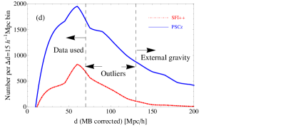
The final result is a linear model for the peculiar velocity field specified at the reconstructed real space position of 8,995 PSC galaxies within that were not collapsed into galaxy clusters. Their distribution as a function of distance is plotted in panel (d) of Fig. 1 (blue curve). The vertical line at indicates the volume considered in the – comparisons (‘Data used’ in Table 1) and the vertical line at separates objects with predicted velocities not used in the quantitative analysis (‘Outliers’) from those used to model the gravitational pull of distant structures.
To compare predicted and observed velocities we need to interpolate model velocities at the positions of galaxies in the peculiar velocity catalogues. This is done by applying a Gaussian kernel of the same radius to the predicted 3D velocity specified at the position of the PSC galaxies, , i.e.
| (2) |
where the sum runs over the PSC galaxies and is the position of the galaxy in the peculiar velocity catalogue. Interpolated velocities are projected along the line of sight, , in order to be compared to the measured ones.
After correcting for systematic errors, the typical random errors on predicted velocities, estimated from mock PSC galaxy catalogs, is (, 1999). These errors are much smaller than those in the measured velocities and therefore will be neglected in the – comparison presented in this work.
3 Observed peculiar velocities
Measured peculiar velocities are the other ingredient of the – comparison. In this work we consider four catalogues (ENEAR, SN, SFI++ and A1SN) that we briefly describe below. We restrict our attention to these catalogues for two reasons. First, they are high quality, recently assembled data sets that densely sample the peculiar velocity field in the local Universe. Second, peculiar velocities are estimated from different distance indicators. These two features minimise the chance of systematic errors and thus allow us to perform a joint analysis, reducing random errors considerably.
There are additional velocity catalogues (SC, 1998, 1999), (SMAC, 1999a, 2004), (EFAR 2001), and (Willick 1999) that have been recently used to estimate the bulk flow in the local Universe (e.g. (2009, 2010)). While these other catalogues can be useful to measure averaged quantities like the bulk flow, they are too sparse and noisy to improve the constrains on from a point-by-point comparison, like in the – analysis. To verify this prejudice we did include them in our analysis and found no improvement in the estimate. For this reason they are not included in the analysis presented here. The four catalogues we use are described as follows:
-
1.
ENEAR. This is a survey of Fundamental Plane distances to nearby 697 early-type galaxies (, 2000; Bernardi et al., 2002; , 2003), either isolated or in groups. Typical errors for the isolated objects are per cent of their distance. The characteristic depth111The characteristic depth of each catalogue is defined as the error-weighted depth , where , is the measurement error of line-of-sight velocity (, 2009, 2010, 2011, 2012) of this sample is .
-
2.
SN. This sample consists of 103 Type Ia supernovae taken from the compilation of (2003). These objects are good standard candles and their distances are estimated more accurately ( per cent) than in the previous case. The characteristic depth of the survey is .
-
3.
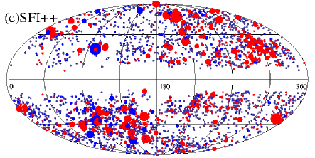
SFI++. This is the largest and densest survey of peculiar velocities available to date (, 2007). The sample considered here consists of 3456 late-type galaxies with peculiar velocities derived from the Tully-Fisher relation. The majority of these objects are in the field (2675) and the rest found in groups (726). Their distribution across the sky is remarkably homogeneous, as shown in panel (c) of Fig. 1. Their radial distribution (red curve in panel (d) of the same figure), looks like a scaled-down version of that of the PSC galaxies. The characteristic depth of SFI++ is around . Typical errors are of the order of per cent. Unlike for other cases, the estimated peculiar velocities in the catalogue have been already corrected for Malmquist bias (, 2007).
-
4.
A1SN. This catalogue, also known as the ‘First Amendment’ supernovae sample, contains 245 Type Ia supernovae (, 2012). It was obtained by merging three data sets: (1) a sample of 106 objects from (2007) and (2009), (2) a collection of 113 objects by (2009), and (3) 28 objects from the ‘Carnegie Supernovae project’ (, 2010). The characteristic depth of the whole catalogue is , significantly larger than that of the other catalogues. Typical errors are of the order of per cent.
| ENEAR | ||
|---|---|---|
| SN | ||
| SFI++ | ||
| A1SN |
In Table 1 we list the number of objects is each catalogue. Only those within , indicated in column 2, are considered for the – comparison. At larger distances the sampling of the underlying velocity field becomes very sparse and random errors too large. Indeed, when we include ‘outliers’ in the range (–) (column 3) the scatter among the values obtained from the different catalogues increases, hinting at possible systematic errors in either predicted or measured peculiar velocities. Finally, since we perform the – comparison in the Local Group frame, velocities in the catalogues that are provided in the CMB frame are transformed to the Local Group frame by subtracting the line of sight component of the Local Group velocity determined from the CMB dipole toward (Scott & Smoot, 2010).
3.1 Malmquist bias correction
Peculiar velocities in these catalogues are potentially prone to Malmquist bias (MB) since they were estimated (1) through ‘forward’ application of the distance indicator, i.e. by estimating a distance-dependent quantity from a distance-independent one and (2) under the assumption that the estimated distance is the the best estimate of the true one (, 1995). Of all catalogues considered here only the SFI++ corrects for MB (, 2007). In all other cases we performed our own correction using the procedure outlined below:
Let us consider the probability distribution of true distance given the distance inferred from the distance indicator and its error (, 1988, 1995):
| (3) |
where is the mass density along the radial direction and is the fractional distance uncertainty of the distance indicators. This conditional probability function can be used to guess the true distance of an object from its estimated distance , if the the density field along the line of sight to the objects, , is known a priori. A popular approach is to assume that is constant and the resulting analytic expression is known as homogeneous MB. However, is far from being constant, even on the smoothing scales of the model velocity field, and to correct for the homogeneous MB we need to follow a different strategy.
The key issue is to model . We do this using the very same velocity model of Section 2. More precisely, we use the real-space reconstructed positions of the PSC galaxies as mass tracers to interpolate the mass density field on a cubic grid of and mesh size , smoothed with a Gaussian filter of . The field on the lattice is then interpolated along the line of sight to each object, galaxies and Type Ia supernovae alike. The value of along the line of sight is specified at the position of 21 equally-spaced points, with a binning of . Finally, Eq. (3) is used to predict from using a MonteCarlo rejection procedure.
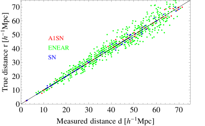
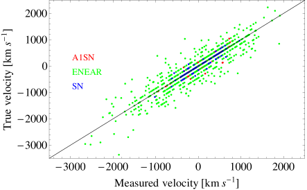
The MB correction is applied to all objects in the catalogues, apart from SFI++ galaxies. In Fig. 2, we compare the measured distance (-axis, before MB correction) and the estimated true distance (-axis, after MonteCarlo, MB correction). Removing this bias preferentially places galaxies at larger distances. The magnitude of the effect is quantified by the scatter of the points around the black line. It depends on the amplitude of the measured velocity error and therefore it increases with the distance and is smaller for Type Ia SN. The dispersion around the black line is not symmetric and indicates that, when averaged over many directions, errors in the observed velocities preferentially scatter objects to larger distances.
4 The – comparison method
We are now in the position of comparing observed and model peculiar velocities at the estimated ‘true’ distances to measure the value of .
We compare the observed peculiar velocities of all objects in all velocity catalogues with the theoretical predictions. The latter were basically obtained from Eq. (1) and therefore are sensitive to the mass distribution traced by PSC galaxies out to . However, since the selection function of the catalogue drops beyond , predicted velocities basically probe the mass distribution (and the value of ) within this range. Observed velocities are potentially sensitive to mass inhomogeneities on much larger scales. However, the fact that we perform our comparison in the LG frame essentially eliminates the gravitational pull from scales larger than . Therefore, the – comparisons at all points within effectively probe on scales between the smoothing scale ( Gaussian) and the effective size of the PSC survey (). In this regard, – comparisons are complementary to analyses that are based on multipole decomposition of the observed velocity field (e.g. 2009, 2010) which, instead, are sensitive to the mass distribution on scales larger than that of the peculiar velocity survey.
The error budget in quantitative – comparisons is dominated by uncertainties in the measured velocity. These errors increase with distance and depend on the distant indicator used and therefore may vary considerably from catalogue to catalogue. In addition, different data sets are potentially prone to different systematic errors in the calibration and in the application of the distance indicator. If the goal is to perform a joint – comparison, then these differences need to be properly accounted for. This can be done by adopting the Bayesian hyper-parameter method, which is designed to objectively assess whether different errors in different catalogues are properly accounted for. The hyper-parameter approach is designed to scale the errors of the data sets, and then marginalise over all other parameters to obtain an estimate of the relative statistical ‘weight’ of the different data sets. In practice, a conventional is defined as , where and are the observed quantity and its measurement error, and is the corresponding theoretical value with parameters . Then the hyper-parameter effectively scales the errors as . Therefore, by marginalising over the other free parameters, one can compute the distribution of , which gives an objective diagnostic of whether the data sets are problematic and hence deserve further study of the systematic or random errors (, 2000).
Joint analyses of different velocity catalogues have been recently performed to investigate the bulk flow, or higher moments of the cosmic velocity field in the local Universe (, 2009, 2010). When combining various data sets the main issue is the freedom in assigning the relative weights of different measurements. The standard way of combining two different data sets (A and B) is by minimising the total defined as (, 2000, 2002)
| (4) |
This procedure assumes that one can trust the estimated random errors, so that the individual statistics have equal weights. However, when combining two or more different data sets with different errors, one may want to assign different weights to the individual statistics
| (5) |
where and are the Lagrangian multipliers that constitute the Bayesian hyper-parameters. Therefore, even if the measurement errors are inaccurate, the hyper-parameters can assess the relative weight of different experiments, and hence let the experiments objectively determine their own weights.
In the Bayesian hyper-parameter method framework , the a posteriori distribution of the parameter is defined as (, 2000)
| (6) |
where represents the data, the sum is over all data sets, is the number of data in each data set and is the of the th data set (see 2002 and Appendix B of 2010 for detailed discussions).
In this work we define the for each velocity catalogue as
| (7) |
where is the measurement error for the line-of-sight peculiar velocity , and is the hyper-parameter of the catalogue. Model velocities are normalised to and linearly scaled by the free parameter according to Eq. (1). Then the likelihood function becomes
| (8) |
Note that this is the likelihood of each individual catalogue characterized by its hyper-parameter that represents the (unknown) scaling of measurement error. The distribution of for the single catalogue can be obtained by marginalise the likelihood in Eq. (8) over and vice versa.
In contrast, Eq. (6) defines the posterior probability of the hyper-parameters and given a combination of different data sets . It is obtained from the combination of likelihoods of the different catalogues in Eq. (8). The distribution of from the joint analysis is obtained by minimising Eq. (6) with respect to .
5 Results
In this section we present the results obtained from the hyper-parameter method, investigate the – comparisons separately for each catalogue and assess the goodness of the fit by analysing the correlation among the residuals in the comparisons.
5.1 value and hyper-parameters
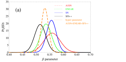
The results of the hyper-parameter analysis are summarised in the top panels of Fig. 3. Panel (a), on the left, shows the posterior probability of the value obtained form each velocity catalogue after marginalising over the corresponding hyper-parameter . Different colours refer to different catalogues, indicated by the labels. SFI++ galaxies prefer a lower value of , whereas the distribution of both Type Ia supernovae catalogues peak at larger values. However, the overlap among the different probability distributions is significant, indicating that the values obtained from the different – comparisons agree with each other.
This impression is confirmed in Table 2, where we list the values of at the peak of the various distributions, together with the width of their Gaussian distributions (column 2). For comparison we also list the values obtained from – comparisons based on the same velocity catalogues. (column 4 in Table 2). They are listed only for reference, since a quantitative comparison should account for the different model velocity fields, comparison techniques and objects considered in each analysis. No – comparison was performed with the SFI++ velocities.
In Fig. 3 the orange curve that peaks at is the result of combining all catalogues in the joint hyper-parameter analysis. The fact that the distribution largely overlaps with those obtained for the individual catalogues confirms the consistency among the results and allows us to estimate with a per cent error. This constraint is remarkably tight, but we have to keep in mind that we are assuming here that errors are solely contributed by uncertainties in measured velocities, and that all other possible sources, including cosmic variance, can be safely neglected.
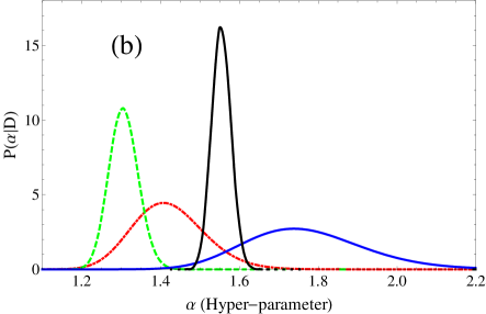
In panel (b) of Fig. 3, we plot the marginalised distribution of hyper-parameter for the four catalogues. Their values are listed in column 5 of Table 2. The fact that is larger than unity for all subsets suggests that random errors have been systematically underestimated by a factor . In our analysis we have assumed that the error budget is dominated by uncertainties in measured peculiar velocities and have ignored errors in the velocity model. We’ve justified this assumption in Section 2 based on the mock catalogue analysis performed by (, 1999, 2001). Another error source that we have neglected is associated to the procedure adopted to correct for the Malmquist bias. To check whether this can indeed account for the remaining error we have performed Montecarlo realization of the MB correction and evaluate its uncertainties from the scatter in the value of . We have done this exercise for the ENEAR catalogue and found that the MB correction induces an error of the same size as the one from measured velocities. When the two are added in quadrature the total error increases by a factor , consistent with the hyper-parameters valued.
We conclude that errors on are contributed by uncertainties in the measured velocities and in the MB corrections and that, for each velocity catalogue, the latter can be estimated scaling the former by the hyper parameter . All errors quoted in Table 2 have been estimated in this way.
5.2 Individual – comparisons
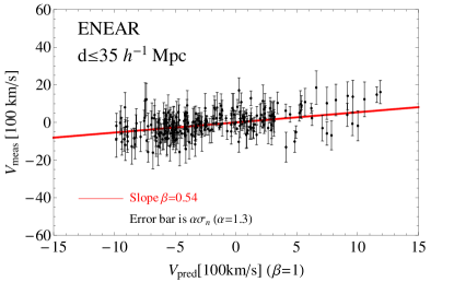
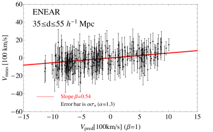
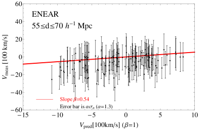
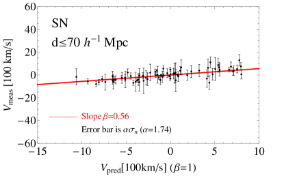
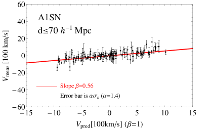
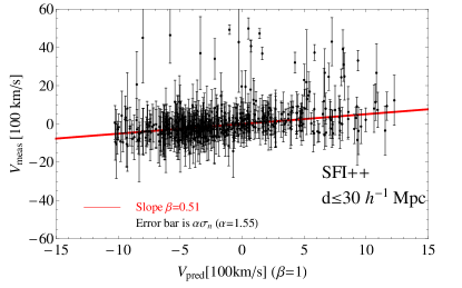
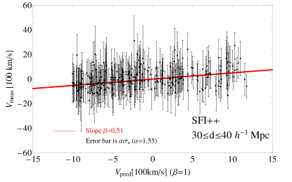
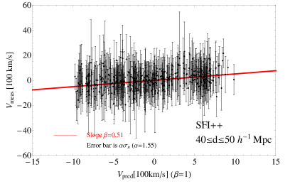
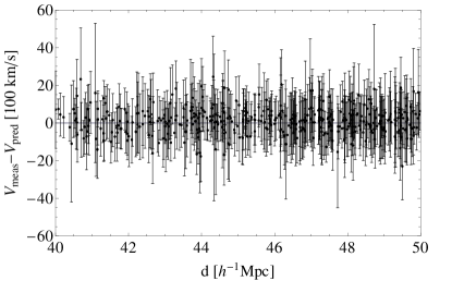
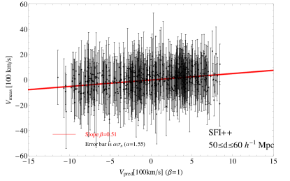
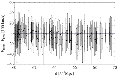
Let us now investigate how well predicted peculiar velocities match the observed ones in each catalogue. We do this by comparing model predictions to observations on a point-by-point basis. The results are the scatter plots shown in the left panels of Figs. 4 to 8. One point in each plot indicates an object in one catalogue. Observed velocities are on the -axis and predicted velocities normalised to are indicated on the -axis. Error bars represent 1 uncertainties in the measured velocities multiplied by the hyper-parameter of the catalogue, as indicated in Table 2. Straight lines represent the best fit value of from the hyper-parameter analysis with a slope also listed in Table 2. Panels on the right show the velocity residuals computed at the estimated ‘true’ distance of the object. For those catalogues that contain a sufficiently large number of objects, we break down the comparison by distance and show the – scatter plots for objects in different spherical shells.
-
1.
ENEAR catalogue. In Fig. 4 we show the – comparisons for objects in three different distance intervals. In the innermost shell () the general agreement between observed and predicted velocities is quite good. The few objects that show significant departures from the best fit are typically found beyond and have positive predicted velocities. Similar residuals are also seen in the ENEAR-PSC velocity maps of (2001) and are mostly galaxies infalling in the Hydra-Centaurus direction and outflowing from the Perseus-Pisces complex. The Hydra-Centaurus infall is attributed to the Great Attractor, an overdensity originally estimated to have a mass of located at (, 1988), subsequently corrected to and () (, 2000). The absence of large velocity residuals in this shell indicates that this prominent infall is well reproduced by the model velocity field. This agreement persists out to , i.e. in the second shell, meaning that the possible backside infall to the Great Attractor is also correctly predicted by the model.
Measured peculiar velocities in the outermost shell are, on average, larger than model predictions. As anticipated, the accuracy of the velocity model decreases with distance because distant structures are poorly sampled by galaxies in the flux-limited PSC catalogue. One example is the Shapley concentration, a large complex of clusters whose dynamical relevance has been outlined by many authors (e.g. 1989, 1999b, 1999). However, a poor sampling of this supercluster would lead to an underestimate of the predicted velocities, whereas here we have the opposite effect. The systematic trend observed in the scatter plot would rather be explained by the poor sampling of low density regions, i.e. large super-voids. Alternatively, these negative residuals could reflect the fact that our model velocity field relies on linear theory and therefore tends to overestimate peculiar velocities near the peaks of the density field, which in turn at large distances could be artificially boosted up by shot noise (, 2000). Whatever the reason, it is worth pointing out that negative velocity residuals of the same amplitude were also found by (2001) for ENEAR galaxies at similar distances and concentrated in the area and .
-
2.
SN and A1SN catalogues. The – comparisons of the objects in both catalogues shown in Figs. 5 and 6 indicate a good match between model predictions and observed peculiar velocities. This agreement is particularly impressive considering the comparatively smaller errors in the measured supernova velocities. This result highlights the fact that Type Ia supernova samples are effective probes of the underlying density field and should be considered as a serious alternative to galaxy-based, peculiar velocity catalogues.
-
3.
SFI++ catalogues. In this case we show the – scatter plots for objects in five different shells. Errors become progressively larger with distance, having little statistical significance in the outer shell.
In the innermost shells we notice the presence of several discrepant data points, characterised by extremely large peculiar velocities, all of them outgoing. No other object in any other catalogues or in the more external shells has measured velocities of the same magnitude. Note that for SFI++ galaxies we did not perform our MB correction, but rely on the built-in MB corrections. Therefore, the features of large velocities may suggest an inadequate correction for the inhomogeneous MB. This is quite challenging since in the very local region in which the redshift surveys are used to trace the density field are often incomplete.
Finally, in the outermost shells we see that residuals become systematically more negative, in analogy to what we see in the ENEAR catalogue. Explanations proposed to account for that behavior are also valid here.









5.3 Analysis of the velocity residuals


The Bayesian, hyper-parameter analysis determines the best value that characterises our model velocity field but cannot address the question of whether or not the model provide an adequate fit to the observed velocities. Inadequate fits typically generate spurious correlations in the velocity residuals. Here we follow (1997, 1998) and (2001) and look for anomalous spatial correlation in the – residual maps.
First, we define the normalised velocity residual as
| (9) |
for each galaxy in the catalogue. This quantity depends on the free parameter and, when averaged over all objects in the catalogues, is minimised by the corresponding best fit values in Table 2. Then, we consider all pairs of galaxies in the catalogue and compute the two-point correlation function for the velocity residuals:
| (10) |
where is the number of galaxy pairs within predicted separation and the sum runs over all pairs . If the model velocity field provides a good match with the observed velocities then residuals should be spatially uncorrelated. In contrast, correlated residuals indicate the presence of systematic effects on some scale.
Normalised velocity residuals and their correlation function have been computed for all objects in the catalogues and for values of in the range in steps of . As an example in Fig. 9 we show the correlation function of the velocity residuals, , for all ENEAR galaxies with separations . The three panels refer to different values of specified by the labels, including the best-fit value (central panel). Error bars represent Poisson noise, . It is clear form the plots that the best fit model behaves much better that the two other cases explored, in which residuals are significantly correlated (or anti-correlated) at almost all separations. Focusing on the case we see that the value of is consistent with the null hypothesis of no correlation over most of the distance bins. The excess correlation at small scales reflects the fact that the model velocity field is smoothed with a Gaussian filter of radius . The residual correlation functions of all other catalogues are similar to those of the ENEAR galaxies and therefore are not shown here.
To quantify the goodness of fits we compute the following quantity (, 2001)
| (11) |
where , and is the number of bins in which we compute . (1997) showed that if residuals are uncorrelated then behaves like a Gaussian random variable with zero mean and variable , and that the is distributed like a function with a number of degrees of freedom equal to , where the factor , computed from mock catalogues, accounts for the correlation among the bins.
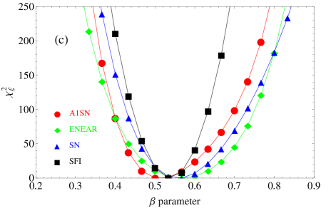
We have computed as a function of for all velocity catalogues. Results are shown in panel (c) of Fig. 3. Different symbols and colours represent different velocity catalogues, indicated by the labels. To ease the comparison we set the minimum of equal to zero for all curves. The distributions are remarkably similar, with minima very close to each other and in agreement with the best fit value of . This result is by no means trivial and indicate that the PSC linear velocity model with provides an adequate fit to the peculiar velocities of very different types of objects from different catalogues. To quantify the agreement we exploit the fact that obeys statistics and use this fact to compute a formal 1 error from . The results of this exercise are listed in column 3 of Table 2 and confirm the qualitative agreement found from the visual inspection.
6 Discussion and Conclusion
In this work we used the PSC galaxy redshift catalogue to predict the cosmic velocity field in the local Universe within the framework of gravitational instability and assuming linear theory and linear biasing. The model velocity field, which depends on a single parameter , is compared to the observed velocities of different types of objects in the ENEAR, SN, SFI++ and A1SN catalogues. We restrict our comparison to objects within , where errors on measured velocities are reasonably small and we can trust the model velocity field. Great care has been taken in correcting for the inhomogeneous Malmquist bias. This is done by using PSC to trace the underlying mass density field and by adopting a Monte Carlo rejection procedure to statistically correct for the MB. Finally, model and observed velocities have been compared in a Bayesian framework using the hyper-parameter method. This technique is designed to estimate the statistical weights of different data set in an objective way and allows one to jointly analyse different velocity catalogues. Here are the main results of our analysis.
-
1.
The hyper-parameter – comparisons performed for each catalogue give values that are consistent within the errors. This means that the single velocity model is a best fit to all data sets. In addition, the best fit values for the ENEAR, SN and A1SN catalogues agree with those obtained from previous – comparisons that used the same data sets but different velocity models and comparison techniques.
-
2.
The joint – comparison performed with the hyper-parameter technique using all data sets significantly improves the accuracy in the estimate of . The best fit value is .
This result can be used to set a constraint on the growth rate of density fluctuations at , i.e. . The value of this quantity is sensitive to the expansion history of the Universe. Its measurement will allow us to understand whether the current cosmic acceleration is driven by a Dark Energy component or perhaps general relativity theory needs modification on cosmological scales. Most of the current estimates have been performed at moderate redshift by quantifying the apparent anisotropies in the clustering of galaxies induced by redshift space distortions (RSD, 2004, 2006, 2008, 2009, 2011, 2012, 2012, 2012). Indeed one of the main goals of ongoing (Drinkwater et al. 2010; Eisenstein et al. 2011; Guzzo et al., in preparation) and planned (Schlegel et al., 2011; Laureijs et al., 2011) redshift surveys is to measure the growth rate at higher redshift, to increase the -baseline for this cosmological test. As pointed out for example by (2012), the additional estimates at can sharpen the observational constraints. Moreover, at the growth rate can be estimated using techniques alternative to RSD, hence providing an important cross-check among the methods.
In Table 3 we list the most recent estimate of , the growth rate normalised to the rms mass density fluctuation on scales. The last entry is the value obtained from our analysis computed as , where is the rms fluctuation in the number density of PSC galaxies (, 2002). This result agrees with CDM model predictions. All estimates in Table 3 are in reasonably good agreement. The largest discrepancy is below 2 significance.
-
3.
Hyper-parameters. From the hyper-parameter analyses of the – comparison and after marginalising over we obtain the hyper-parameters of the different data sets. We find that all of them are slightly larger but quite close to unity, which indicates that velocity errors are slightly overestimated in all velocity catalogues, possibly reflecting the fact that in our analysis we did not include uncertainties in the MB correction.
-
4.
– scatter plots. The inspection of the – comparison on a point-by-point basis from scatter plots reveals that, on average, the model velocity field provides a good fit to observed peculiar velocities in all catalogues. The agreement is especially remarkable for the case of Type Ia supernovae that have much smaller velocity errors and constitutes an important check for the gravitational instability scenario.
The only exceptions are distant ENEAR and SFI++ galaxies, for which model prediction systematically overestimate observed velocities. A similar systematic was seen in a previous ENEAR vs. PSC comparison (, 2001), mainly for galaxies in the region and . Among the possible explanations is the possible poor sampling of distant inhomogeneities or inaccurate modelling of the flow around distant density peaks. Additionally, a few nearby SFI++ galaxies have peculiar velocities that are very large and cannot be matched by model predictions. This might just reflect uncertainties in the original correction for inhomogeneous Malmquist bias which, in the local volume, is notoriously difficult to model due to the incompleteness in the parent redshift catalogues.
-
5.
Goodness of the fit. To evaluate whether our best fit model velocity field is also a good model we searched for spurious correlations among velocity residuals. We have considered all object pairs with separations up to . Apart from a positive correlation signal at small separations, induced by the Gaussian window used to filter out non-linear effects, when we set equal to its best fit value we find that the residual correlation function is consistent with zero. This result further confirms the adequacy of the velocity model and the validity of the gravitational instability picture.
Although the study of the peculiar velocity field is still very data-limited, future surveys, e.g. the 6dF survey (, 2009), or eventually using the 21 cm line, e.g. with the , may provide rich resources for the study of large-scale structure and cosmic flows. But even with these large data-sets, it will still be important to carefully assess the potential systematics.
Acknowledgments: We would like to thank George Efstathiou and Jeremiah Ostriker for helpful discussions, and Michael Hudson and Stephen Turnbull for sharing A1SN catalogue. YZM is supported by a CITA National Fellowship. This research is supported by the Natural Science and Engineering Research Council of Canada.
References
- Bernardi et al. (2002) Bernardi M., Alonso M. V., da Costa L. N., Willmer C. N. A., Wegner G., Pellegrini P. S., Rite C., Maia M. A. G., 2002, AJ, 123, 2990
- (2) Beutler F., et al., 2012, MNRAS, 423, 3430
- (3) Blake C., et al., 2011, MNRAS, 415, 2876
- (4) Branchini E., 2001, MNRAS, 326, 1191
- (5) Branchini E., et al., 1999, MNRAS, 308, 1
- (6) Branchini E., Zehavi I., Plionis M., Dekel A., 2000, MNRAS, 313, 491
- (7) Branchini E., Davis M., Nusser A., 2012, MNRAS, 424, 472
- (8) Colless M., Saglia R. P., Burstein D., Davis R. L., McMahan R. K., Wegner G., 2001, MNRAS, 321, 277
- (9) da Costa L. N., Nusser A., Freudling W., Giovanelli R., Haynes M. P., Salzer J. J., Wegner G., 1998, MNRAS, 299, 425
- (10) da Costa L. N., Bernardi M., Alonso M. V., Wegner G., Willmer, C. N. A., Pellegrini P. S., Rit C., Maia M. A. G., 2000, AJ, 120, 95
- (11) Dale D. A., Giovanelli R., Haynes M. P., Campusano L. E., Hardy E., 1999, AJ, 118, 1489
- (12) Davis M., Nusser A.; Willick J. A., 1996, ApJ, 473, 22
- (13) Davis M., Nusser A., Masters K. L., Springob C., Huchra J. P., Lemson G., 2011, MNRAS, 413, 2906
- Drinkwater et al. (2010) Drinkwater M. J., et al., 2010, MNRAS, 401, 1429
- Eisenstein et al. (2011) Eisenstein D. J., et al., 2011, AJ, 142, 72
- (16) Folatelli G. et al., 2010, AJ, 139, 120
- (17) Feldman H. A., Frieman J. A., Fry J. N., Scoccimarro R., 2001, Phys. Rev. Lett., 86, 1434
- (18) Feldman H., Watkins R., Hudson M. J., 2010, MNRAS, 407, 2328
- (19) Fisher K., Huchra J., Strauss M., Davis M., Yahil A., Schlegel D., 1995, ApJ, 100, 69
- (20) Giovanelli R., Haynes M. P., Herter T., Vogt N. P., Wegner G., Salzer J. J., da Costa L. N., Freudling W., 1997, AJ, 113, 22
- (21) Giovanelli R., Haynes M. P., Salzer J. J., Wegner G., da Costa L. N., Freudling W., 1998, AJ, 116, 2632
- (22) Guzzo L., et al., 2008, Nat, 541, 541
- (23) Hamilton A.J.S., and Tegmark M., 2002, MNRAS, 330, 506
- (24) Haynes M. et al., 1999, Astron. J., 117, 2039
- (25) Hicken M. et al., 2009, ApJ, 700, 1097
- (26) Hobson M.P., Bridle S.L., Lahav O., 2002, MNRAS, 335, 377
- (27) Huchra J.P., et al., 2012, ApJS, 199, 26
- (28) Hudson M. J., 1994, MNRAS, 266, 468
- (29) Hudson M. J., 1999a, PASP, 111, 57
- (30) Hudson M. J., 1999b, ApJL, 512, 59
- (31) Hudson M.J., Smith R.J.,Lucey J. R., Branchini E., 2004, MNRAS, 352, 61
- (32) Hudson M.J., Turnbull S., 2012, ApJ, 751L, 30
- (33) Jha S., Riess A. G., Kirshner R. P., 2007, ApJ, 659, 122
- (34) Jones D. H., et. al, 2009, MNRAS, 399, 683
- (35) Kaiser N., Lahav, O.,1989, MNRAS, 237, 129
- (36) Lahav O., Bridle S. L., Hobson M. P., Lasenby A. N., Sodre L., 2000, MNRAS, 315, 45
- Laureijs et al. (2011) Laureijs R., et al., 2011, arXiv:1110.3193
- (38) Linder E. V., 2005, Phys. Rev. D., 72, 043529
- (39) Lynden-Bell D., Faber S. M., Burstein D., Davis R. L., Dressler A., Terlevich R.J., Wegner G., 1988, ApJ, 326, 19
- (40) Ma Y. Z., Zhao W., Brown M. L., 2010, JCAP, 1010, 007
- (41) Ma Y.Z., Ostriker J., Zhao G.B., 2012, JCAP, 6, 26
- (42) Malmquist K. G., 1920 Medd. Lund. Astron. Obs., Ser II, 22, 1
- (43) Masters K. L., Springob C. M., Haynes M. P., Giovanelli R., 2006, ApJ, 653, 861
- (44) Nusser A., da Costa L. N., Branchini E., Bernardi M., Alonso M. V., Wegner G., Willmer C. N. A., Pellegrini P. S., 2001, MNRAS, 320, L21
- (45) Nusser A., Branchini E., Davis M., 2011, ApJ, 735, 77
- (46) Peebles P. J. E., Physical Cosmology. Princeton University Press, 1971
- (47) Peebles P. J. E., Principles of Physical Cosmology. Princeton University Press, 1993
- (48) Percival W. J., et al., 2004, MNRAS, 353, 1201
- (49) Pike R. W., Hudson M. J., 2005, ApJ, 635, 11
- (50) Radburn-Smith D.J., Lucey J.R., Hudon M.J., 2004, MNRAS, 355, 1378
- (51) Reid B. A., 2012 1203.6641 [arXiv:astro-ph]
- (52) Samushia L., Percival W. J., Raccanelli A., 2012, MNRAS, 420, 2102
- (53) Saunders W., et al., 2000, MNRAS, 317, 55
- (54) Scaramella R., Baiesi-Pillastrini G., Chincarini G., Vettolani G., Zamorani G., 1989, Nature, 338 652
- Schlegel et al. (2011) Schlegel D., et al., 2011, arXiv:1106.1706
- (56) Scoccimarro R., Feldman H. A., Fry J. N., Frieman J. A., 2001, ApJ, 546, 652
- Scott & Smoot (2010) Scott D., Smoot G., 2010 Review of Particle Physics, 1005.0555 [arXiv:astro-ph]
- Skrutskie et al. (2006) Skrutskie M. F., et al., 2006, AJ, 131, 1163
- (59) Square Kilometre Array: http://www.skatelescope.org
- (60) Springob C. M., Masters K. L., Haynes M. P., Giovanelli R., Marinoni C., 2007, ApJS, 172, 599
- (61) Song Y.-S., Percival W. J., 2009, JCAP, 10, 4
- (62) Strauss M. A., Willick J. A., 1995, Phys. Rep., 261, 271
- (63) Tegmark M., et al., 2006, Phys. Rev. D, 74, 123507
- (64) Tojeiro R., et al., 2012 MNRAS, tmp 3331T
- (65) Tonry J L., Blakeslee J. P., Ajhar E. A., Dressler A., 2000, ApJ, 530, 625
- (66) Tonry J. L. et al., 2003, ApJ, 594, 1
- (67) Turnbull S. J., Hudson M. J., Feldman H. A., Hicken M., Kirshner R. P., Watkins R., 2012, MNRAS, 420, 447
- (68) Verde L. et al., 2002, MNRAS, 335, 432
- (69) Watkins R., Feldman H. A., Hudson M. J., 2009, MNRAS, 392, 743
- (70) Wenger G. et al., 2003, Astron. J, 126, 2268
- (71) Willick J. A., Strauss M. A., Dekel A., Kolatt T., 1997, ApJ, 486, 629
- (72) Willick J. A., Strauss M. A., 1998, ApJ, 507, 46
- (73) Willick J. A., 1999, ApJ, 522, 647
- (74) Yahil A., Strauss M.A., Davis M., Huchra J.P., 1991, ApJ, 372, 380
- (75) Zaroubi S., Branchini E., Hoffman Y., da Costa L.N., 2002, MNRAS, 336, 1234