Optimal hypothesis testing for high dimensional covariance matrices

Abstract

This paper considers testing a covariance matrix $\Sigma$ in the high dimensional setting where the dimension $p$ can be comparable or much larger than the sample size $n$. The problem of testing the hypothesis $H_{0}\mathchoice{\nobreak\,\colon}{\nobreak\,\colon}{\nobreak\,\colon\;}{\nobreak\,\colon\;}\Sigma=\Sigma_{0}$ for a given covariance matrix $\Sigma_{0}$ is studied from a minimax point of view. We first characterize the boundary that separates the testable region from the non-testable region by the Frobenius norm when the ratio between the dimension $p$ over the sample size $n$ is bounded. A test based on a $U$-statistic is introduced and is shown to be rate optimal over this asymptotic regime. Furthermore, it is shown that the power of this test uniformly dominates that of the corrected likelihood ratio test (CLRT) over the entire asymptotic regime under which the CLRT is applicable. The power of the $U$-statistic based test is also analyzed when $p/n$ is unbounded.

and

1 Introduction

Covariance structure plays a fundamental role in multivariate analysis and testing the covariance matrix is an important problem. Let $X_{1},\dots,X_{n}$ be $n$ independent and identically distributed $p$-vectors following a multivariate normal distribution $N_{p}(0,\Sigma)$. A hypothesis testing problem of significant interest is testing

$$H_{0}\colon\ \Sigma=I.$$ (1)

Note that any null hypothesis $H_{0}\colon\ \Sigma=\Sigma_{0}$ with a given positive definite covariance matrix $\Sigma_{0}$ is equivalent to (1), since one can always transform $X_{i}$ to $\tilde{X}_{i}=\Sigma_{0}^{-1/2}X_{i}$ and then test (1) based on the transformed data.

This testing problem has been well studied in the classical setting of small $p$ and large $n$. See, for example, Anderson [1] and Muirhead [13]. In particular, the likelihood ratio test (LRT) is commonly used. Driven by a wide range of contemporary scientific applications, analysis of high dimensional data is of significant current interest. In the high dimensional setting, where the dimension can be comparable to or even much larger than the sample size, the conventional testing procedures such as the LRT perform poorly or are not even well defined. Several testing procedures designed for the high-dimensional setting have been proposed. Let $S=\frac{1}{n}\sum_{i=1}^{n}X_{i}X_{i}^{\prime}$ be the sample covariance matrix. The existing tests for (1) in the literature can be categorized as the following according to the asymptotic regime under which they are suitable:

• $p$ fixed and $n\to\infty$. In this classical asymptotic regime, conventional tests for (1) include the likelihood ratio test (LRT) [1], Roy’s largest root test [16], and Nagao’s test [14]. In particular, the LRT statistic is $\mathit{LR}_{n}=nL_{n}$, where

  $$L_{n}=\operatorname{tr}{S}-\log\operatorname{det}(S)-p.$$

  The asymptotic distribution of $\mathit{LR}_{n}$ under $H_{0}$ is $\chi^{2}_{p(p+1)/2}$.

• Both $n,p\to\infty$ and $p/n\to c\in(0,\infty)$. Investigation in this asymptotic regime has been very active in the past decade. For example, Johnstone [11] revisited Roy’s largest root test and derived the Tracy–Widom limit of its null distribution. Ledoit and Wolf [12] proposed a new test based on Nagao’s proposal. See also Srivastava [17]. When $p$ grows, the chi-squared limiting null distribution of the LRT statistic $\mathit{LR}_{n}$ is no longer valid. Recently, Bai et al. [2] proposed a corrected LRT when $c<1$, and Jiang et al. [10] extended it to the case when $p<n$ and $c=1$. Here, for $c_{n}=p/n$, the test statistic of the corrected LRT is

  $$\mathit{CLR}_{n}=\frac{L_{n}-p[1-(1-c_{n}^{-1})\log(1-c_{n})]-{1}/{2}\log(1-c_{n})}{\sqrt{-2\log(1-c_{n})-2c_{n}}},$$ (2)

  whose asymptotic null distribution is $N(0,1)$. Note that no test based on the likelihood ratio can be defined when $p>n$ or $c>1$.

• Both $n,p\to\infty$ and $p/n\to\infty$. This is the ultra high-dimensional setting and both the LRT and corrected LRT are not well defined in this case. The testing problem in this asymptotic regime is not as well studied as in the previous categories. Birke and Dette [3] derived the asymptotic null distribution of the Ledoit–Wolf test under the current asymptotic regime. More recently, Chen et al. [7] proposed a new test statistic and derived its asymptotic null distribution when both $n,p\to\infty$, regardless of the limiting behavior of $p/n$.

When the dimension $p$ grows together with the sample size $n$, the focus of most of the aforementioned papers is mainly on finding the asymptotic null distribution of the proposed test statistic, so the significance level of the test can be controlled. The few exceptions include Srivastava [17] and Chen et al. [7], where the asymptotic pointwise power of the proposed tests is also studied. Recently, Onatski et al. [15] established the regime of mutual contiguity of the joint distributions of the sample eigenvalues under the null and under the special alternative of rank one perturbation to the identity matrix, and then applied Le Cam’s third lemma to study the pointwise power of a collection of eigenvalue based tests for (1) against this special class of alternative.

In the present paper, we investigate this testing problem in the high-dimensional settings from a minimax point of view. Consider testing (1) against a composite alternative hypothesis

$$H_{1}\colon\ \Sigma\in\Theta,\qquad\mbox{where }\Theta=\Theta_{n}=\bigl{\{}\Sigma\colon\ \|\Sigma-I\|_{F}\geq\varepsilon_{n}\bigr{\}}.$$ (3)

Here, $\|A\|_{F}=(\sum_{ij}a_{ij}^{2})^{1/2}$ denotes the Frobenius norm of a matrix $A=(a_{ij})$. It is clear that the difficulty of testing between $H_{0}$ and $H_{1}$ depends on the value of $\varepsilon_{n}$: the smaller $\varepsilon_{n}$ is, the harder it is to distinguish between the two hypotheses. An interesting question is: What is the boundary that separates the testable region, where it is possible to reliably detect the alternative based on the observations, from the untestable region, where it is impossible to do so? This problem is connected to the classical contiguity theory. It is also important to construct a test that can optimally distinguish between the two hypotheses in the testable region. The high-dimensional settings here include all the cases where the dimension $p=p_{n}\to\infty$ as the sample size $n\to\infty$, and there is no restriction on the limit of $p/n$ unless otherwise stated.

For a given the significance level $0<\alpha<1$, our first goal is to identify the separation rate $\varepsilon_{n}$ at which there exists a test $\phi$ based on the random sample $\{X_{1},\ldots,X_{n}\}$ such that

$$\inf_{\Sigma\in\Theta}\mathsf{P}_{\Sigma}(\phi\mbox{ rejects }H_{0})\geq\beta>\alpha.$$

Hence, the test is able to detect any alternative that is separated away from the null by a certain distance $\varepsilon_{n}$ with a guaranteed power $\beta>\alpha$. Our second goal is to construct such a testing procedure $\phi$.

The major contribution of the current paper is threefold. First, we show that if $p/n$ is bounded, then the rate $\varepsilon_{n}$ needs to be no less than $b\sqrt{p/n}$ for some constant $b$. In addition, it is shown that if $\varepsilon_{n}=b\sqrt{p/n}$, there exists a test $\psi$ of significance level $\alpha$, such that $\lim_{n\to\infty}\inf_{\Theta}\mathsf{P}_{\Sigma}(\mbox{$\psi$ rejects $H_{0}$})>\alpha$, and the power tends to $1$ if $b=b_{n}\to\infty$. The test is motivated by the proposal in Chen et al. [7]. (We use $\psi$ to denote the specific test that we construct, while $\phi$ is used to denote a generic test.) Here, we no longer require $p/n$ to be bounded, and the explicit expression for the asymptotic power of $\psi$ is also given. Moreover, we show that the asymptotic power of $\psi$ on $\Theta_{n}$ uniformly dominates that of the corrected LRT by Bai et al. [2] and Jiang et al. [10] over the entire asymptotic regime under which the corrected LRT is defined, that is, $p<n$ and $p/n\to c\in(0,1]$.

The rest of the paper is organized as the following. In Section 2, after introducing basic notation and definitions, we establish a lower bound of the separation rate $\varepsilon_{n}$. Section 3 introduces the test based on a $U$-statistic and provides a Berry–Essen bound for its weak convergence to the normal limit under both the null and the alternative hypotheses, which leads to the establishment of its guaranteed power over $\Theta$ when $\varepsilon_{n}=b\sqrt{p/n}$. Furthermore, we also show that the power of this test uniformly dominates that of the corrected LRT. The theoretical results are supported by the numerical experiments in Section 4. Further discussions on the connections of our results and those of related testing problems are given in Section 5. The main results are proved in Section 6.

2 Lower bound

In this section, we establish a lower bound for the separation rate $\varepsilon_{n}$ in (3). The result in Section 3 will show that this lower bound is rate-optimal. The lower and upper bounds together characterize the separation boundary between the testable and non-testable regions when the ratio of the dimension $p$ over the sample size $n$ is bounded. This separation boundary can then be used as a minimax benchmark for the evaluation of the performance of a test in this asymptotic regime.

We begin with basic notation and definitions. Throughout the paper, a test $\phi=\phi_{n}(X_{1},\dots,X_{n})$ refers to a measurable function which maps $X_{1},\dots,X_{n}$ to the closed interval $[0,1]$, where the value stands for the probability of rejecting $H_{0}$. So, the significance level of $\phi$ is $\mathsf{P}_{I}(\mbox{$\phi$ rejects $H_{0}$})=\mathsf{E}_{I}\phi$, and its power at a certain alternative $\Sigma$ is $\mathsf{P}_{\Sigma}(\mbox{$\phi$ rejects $H_{0}$})=\mathsf{E}_{\Sigma}\phi$. Here and after, $\mathsf{P}_{\Sigma},\mathsf{E}_{\Sigma},\operatorname{\mathsf{Var}}_{\Sigma}$ and $\operatorname{\mathsf{Cov}}_{\Sigma}$ denote the induced probability measure, expectation, variance and covariance when $X_{1},\dots,X_{n}\stackrel{{\scriptstyle\mathrm{i.i.d.}}}{{\sim}}N_{p}(0,\Sigma)$. The subscript is shown only when clarity dictates.

To state the lower bound result, let $\varepsilon_{n}=b\sqrt{p/n}$ for some constant $b$, and define

$$\Theta(b)=\bigl{\{}\Sigma\colon\ \|\Sigma-I\|_{F}\geq b\sqrt{p/n}\bigr{\}}.$$ (4)

Theorem 1 ((Lower bound))

Let $0<\alpha<\beta<1$. Suppose that as $n\to\infty$, $p\to\infty$ and that $p/n\leq\kappa$ for some constant $\kappa<\infty$ and all $n$. Then there exists a constant $b=b(\kappa,\beta-\alpha)<1$, such that for any test $\phi$ with significance level $\alpha$ for testing $H_{0}\colon\ \Sigma=I$,

$$\limsup_{n\to\infty}\inf_{\Sigma\in\Theta(b)}\mathsf{E}_{\Sigma}\phi<\beta.$$

Theorem 1 shows that no level $\alpha$ test for (1) can distinguish between the two hypotheses with power tending to $1$ as $n$ and $p$ grow, when the separation rate $\varepsilon_{n}$ is of order $\sqrt{p/n}$. Hence, it provides a lower bound for the separation rate.

We now give an outline of the proof for Theorem 1, while the complete proof is provided in Section 6.1. Consider the following “least favorable” subset of $\Theta(b)$:

$$\Theta^{*}(b)=\biggl{\{}\Sigma_{v}=\biggl{[}1-\frac{b}{\sqrt{n(p-1)}}\biggr{]}I_{p\times p}+\frac{b}{\sqrt{n(p-1)}}vv^{\prime}\colon\ v\in\{\pm 1\}^{p}\biggr{\}}.$$ (5)

With slight abuse of notation, let $P_{0}$ be the probability measure when $X_{1},\dots X_{n}\stackrel{{\scriptstyle\mathrm{i.i.d.}}}{{\sim}}N_{p}(0,I)$ and $P_{v}$ the probability measure when $X_{1},\dots,X_{n}\stackrel{{\scriptstyle\mathrm{i.i.d.}}}{{\sim}}N_{p}(0,\Sigma_{v})$. In addition, let $P_{1}=\frac{1}{2^{p}}\sum_{v\in\{\pm 1\}^{p}}P_{v}$ be the average measure of the $P_{v}$’s. Then for any test $\phi$, the sum of probabilities of its two types of errors satisfies

$$\sup_{v}\mathsf{E}_{0}\phi+\mathsf{E}_{v}(1-\phi) \geq \inf_{\psi}\sup_{v}\mathsf{E}_{0}\psi+\mathsf{E}_{v}(1-\psi)$$

$$\geq \inf_{\psi}\frac{1}{2^{p}}\sum_{v}\mathsf{E}_{0}\psi+\mathsf{E}_{v}(1-\psi)$$

$$= \inf_{\psi}\mathsf{E}_{0}\psi+\mathsf{E}_{1}(1-\psi)$$

$$= 1-\frac{1}{2}\|P_{1}-P_{0}\|_{1}.$$

Here, $\mathsf{E}_{0},\mathsf{E}_{v}$ and $\mathsf{E}_{1}$ denote the expectation under $P_{0}$, $P_{v}$ and $P_{1}$ respectively, and $\|P_{1}-P_{0}\|_{1}$ is the $L_{1}$ distance between $P_{0}$ and $P_{1}$. Thus, we obtain

$$\inf_{\Sigma\in\Theta(b)}\mathsf{E}_{\Sigma}\phi\leq\inf_{v}\mathsf{E}_{v}\phi\leq\mathsf{E}_{0}\phi+\frac{1}{2}\|P_{1}-P_{0}\|_{1}=\alpha+\frac{1}{2}\|P_{1}-P_{0}\|_{1}.$$

To control the rightmost side, we bound the $L_{1}$ distance by the chi-square divergence as

$$\|P_{1}-P_{0}\|_{1}^{2}\leq\mathsf{E}_{0}\biggl{|}\frac{\mathrm{d}P_{1}}{\mathrm{d}P_{0}}-1\biggr{|}^{2}=\mathsf{E}_{0}\biggl{|}\frac{\mathrm{d}P_{1}}{\mathrm{d}P_{0}}\biggr{|}^{2}-1=\int\frac{f^{2}_{1}}{f_{0}}-1,$$

where $f_{i}$ is the density function of $P_{i}$ for $i=0,1$. So, the proof can be completed by showing that for an appropriate choice of the constant $b$, one obtains $\int\frac{f_{1}^{2}}{f_{0}}-1\leq 4(\beta-\alpha)^{2}$.

Remark 1.

(a). Note that all the covariance matrices in the least favorable configuration $\Theta^{*}(b)$ defined in (5) have diagonal elements all equal to $1$. Thus, they are also correlation matrices. So the proof of Theorem 1 readily establishes an analogous lower bound result on testing $H_{0}\colon\ R=I$ with $R$ the population correlation matrix.

(b). The lower bound argument here does not extend to the case when $p/n$ is unbounded, because the chi-square divergence becomes unbounded.

3 Upper bound

In this section, we show that there exists a level $\alpha$ test whose power over $\Theta_{n}$ is uniformly larger than a prescribed value $\beta>\alpha$, if $\varepsilon_{n}=b\sqrt{p/n}$ for a large enough constant $b$. This matches the lower bound result in Theorem 1 when $p/n$ is bounded. In addition, the results in the current section remain valid even when $p/n$ is unbounded.

We first introduce the test statistic in Section 3.1, followed by a study on the rate of convergence of its distribution to the normal limit under both the null and the alternative hypotheses in Section 3.2. Section 3.3 then uses the rate of convergence result to study the asymptotic power of the proposed test. Finally, Section 3.4 shows that the test dominates the corrected LRT in (2) when $p/n\to c\in(0,1]$.

3.1 Test statistic

Given a random sample $X_{1},\dots,X_{n}\stackrel{{\scriptstyle\mathrm{i.i.d.}}}{{\sim}}N_{p}(0,\Sigma)$, a natural approach to test between (1) and (3) is to first estimate the squared Frobenius norm $\|\Sigma-I\|_{F}^{2}=\operatorname{tr}(\Sigma-I)^{2}$ by some statistic $T_{n}=T_{n}(X_{1},\dots,X_{n})$, and then reject the null hypothesis if $T_{n}$ is too large. To estimate $\|\Sigma-I\|_{F}^{2}=\operatorname{tr}(\Sigma-I)^{2}$, note that $\mathsf{E}_{\Sigma}h(X_{1},X_{2})=\operatorname{tr}(\Sigma-I)^{2}$ where

$$h(X_{1},X_{2})=\bigl{(}X_{1}^{\prime}X_{2}\bigr{)}^{2}-\bigl{(}X_{1}^{\prime}X_{1}+X_{2}^{\prime}X_{2}\bigr{)}+p.$$ (6)

Therefore, $\operatorname{tr}(\Sigma-I)^{2}$ can be estimated by the following $U$-statistic

$$T_{n}=\frac{2}{n(n-1)}\sum_{1\leq i<j\leq n}h(X_{i},X_{j}),$$ (7)

for which we have

$$\mu_{n}(\Sigma) = \mathsf{E}_{\Sigma}(T_{n})=\operatorname{tr}(\Sigma-I)^{2},$$ (8)

$$\sigma_{n}^{2}(\Sigma) = \operatorname{\mathsf{Var}}_{\Sigma}(T_{n})=\frac{4}{n(n-1)}\bigl{[}\operatorname{tr}^{2}\bigl{(}\Sigma^{2}\bigr{)}+\operatorname{tr}\bigl{(}\Sigma^{4}\bigr{)}\bigr{]}+\frac{8}{n}\operatorname{tr}\bigl{(}\Sigma^{2}(\Sigma-I)^{2}\bigr{)}.$$ (9)

Here, verifying (8) is straightforward, and (9) is proved in Appendix A.2. For the $U$-statistic $T_{n}$, the proof for Theorem 2 of Chen et al. [7] essentially established the following.

Proposition 2 ((Theorem 2 of [7]))

Suppose that $p\to\infty$ as $n\to\infty$. If a sequence of covariance matrices satisfy $\operatorname{tr}(\Sigma^{2})\to\infty$ and $\operatorname{tr}(\Sigma^{4})/\operatorname{tr}^{2}(\Sigma^{2})\to 0$ as $n\to\infty$, then under $\mathsf{P}_{\Sigma}$, we have

$$\frac{T_{n}-\mu_{n}(\Sigma)}{\sigma_{n}(\Sigma)}\Rightarrow N(0,1).$$

Note that as $p\to\infty$, the identity matrix $I_{p\times p}$ satisfies the condition of the above proposition. Also note that $\mu_{n}(I)=0$ and $\sigma_{n}^{2}(I)={4p(p+1)\over n(n-1)}$. Thus, Proposition 2 quantifies the behavior of $T_{n}$ under $H_{0}$, and we could define the test as the following: For any $\alpha\in(0,1)$, an asymptotic level $\alpha$ test based on $T_{n}$ is given by

$$\psi=I\biggl{(}T_{n}>z_{1-\alpha}\cdot 2\sqrt{{p(p+1)\over n(n-1)}}\biggr{)}.$$ (10)

Here, $I(\cdot)$ is the indicator function, and $z_{1-\alpha}$ denotes the $100\times(1-\alpha)$th percentile of the standard normal distribution. This test is motivated by the test introduced in Chen et al. [7], while the original proposal in [7] involves higher order symmetric functions of the $X_{i}$’s.

In addition to specifying the rejection region in (10), Proposition 2 can also be used to study the asymptotic power of $\psi$ over a sequence of simple alternatives. However, to understand the power of $\psi$ over the composite alternative $\Theta$ in (3), it is necessary to understand the rate of convergence of $[T_{n}-\mu_{n}(\Sigma)]/\sigma_{n}(\Sigma)$ to the normal limit, which is the central topic of the next subsection.

3.2 Rate of convergence

We now study the rate of convergence for the distribution of $[T_{n}-\mu_{n}(\Sigma)]/\sigma_{n}(\Sigma)$ to its normal limit in Kolmogorov distance. Let $\Phi(\cdot)$ be the cumulative distribution function of the standard normal distribution. We have the following Berry–Essen type bound.

Proposition 3

Under the condition of Proposition 2, there exists a numeric constant $C$ such that

$$\sup_{x\in\mathbb{R}}\biggl{|}\mathsf{P}_{\Sigma}\biggl{(}\frac{T_{n}-\mu_{n}(\Sigma)}{\sigma_{n}(\Sigma)}\leq x\biggr{)}-\Phi(x)\biggr{|}\leq C\biggl{[}\frac{1}{n}+\frac{\operatorname{tr}(\Sigma^{4})}{\operatorname{tr}^{2}(\Sigma^{2})}\biggr{]}^{1/5}.$$

We outline the proof of Proposition 3 below, while the complete proof is deferred to Section 6.2. The primary tool used in the proof is a Berry–Esseen type bound for martingale central limit theorem by Heyde and Brown [8].

We begin by giving a martingale representation of $T_{n}-\mu_{n}(\Sigma)$. Let $X_{i}\stackrel{{\scriptstyle\mathrm{i.i.d.}}}{{\sim}}N_{p}(0,\Sigma)$. Define filtration

$$\mathcal{F}_{0}=\sigma(\varnothing),\qquad\mathcal{F}_{k}=\sigma(X_{1},\dots,X_{k}),\qquad k=1,\dots,n.$$

Also introducing the notation $\mathsf{E}_{k}[\cdot]=\mathsf{E}_{\Sigma}[\cdot|\mathcal{F}_{k}]$. Then

$$T_{n}-\mu_{n}(\Sigma)=\sum_{k=1}^{n}\mathsf{E}_{k}[T_{n}]-\mathsf{E}_{k-1}[T_{n}]=\sum_{k=1}^{n}D_{nk}.$$ (11)

Here, $\{D_{nk}\colon\ k=1,\dots,n\}$ is a martingale difference sequence. The explicit expression for $D_{nk}$ is

$$D_{nk} = \frac{2}{n(n-1)}\bigl{[}X_{k}^{\prime}Q_{k-1}X_{k}-\operatorname{tr}(Q_{k-1}\Sigma)\bigr{]}$$

$${}+\frac{2}{n}\bigl{[}X_{k}^{\prime}\Sigma X_{k}-\operatorname{tr}\bigl{(}\Sigma^{2}\bigr{)}\bigr{]}-\frac{2}{n}\bigl{[}X_{k}^{\prime}X_{k}-\operatorname{tr}(\Sigma)\bigr{]},$$

with $Q_{k-1}=\sum_{i=1}^{k-1}(X_{i}X_{i}^{\prime}-\Sigma)$. Let $\sigma_{nk}^{2}=\mathsf{E}_{k-1}[D_{nk}^{2}]$, and we have $\sigma_{n}^{2}(\Sigma)=\sum_{k=1}^{n}\mathsf{E}_{\Sigma}[\sigma_{nk}^{2}]$.

Under the current setup, the main theorem in [8] specializes to the following lemma.

Lemma 1

There exist a numeric constant $C$, such that

$$\sup_{x\in\mathbb{R}}\biggl{|}\mathsf{P}_{\Sigma}\biggl{(}\frac{T_{n}-\mu_{n}(\Sigma)}{\sigma_{n}(\Sigma)}\leq x\biggr{)}-\Phi(x)\biggr{|}$$

(13)

$$\quad\leq C\Biggl{[}\frac{1}{\sigma_{n}^{4}(\Sigma)}\Biggl{(}\sum_{k=1}^{n}\mathsf{E}_{\Sigma}\bigl{[}D_{nk}^{4}\bigr{]}+\mathsf{E}_{\Sigma}\Biggl{[}\sum_{k=1}^{n}\sigma_{nk}^{2}-\sigma_{n}^{2}(\Sigma)\Biggr{]}^{2}\Biggr{)}\Biggr{]}^{1/5}.$$

Define

$$E_{1}=\sum_{k=1}^{n}\mathsf{E}_{\Sigma}\bigl{[}D_{nk}^{4}\bigr{]}\quad\mbox{and}\quad E_{2}=\mathsf{E}_{\Sigma}\Biggl{[}\sum_{k=1}^{n}\sigma_{nk}^{2}-\sigma_{n}^{2}(\Sigma)\Biggr{]}^{2}.$$ (14)

The proof of Proposition 3 could then be completed by showing that $E_{1}/\sigma_{n}^{4}(\Sigma)=\mathrm{O}(1/n)$ and $E_{2}/\sigma_{n}^{4}(\Sigma)=\mathrm{O}(\operatorname{tr}(\Sigma^{4})/\operatorname{tr}^{2}(\Sigma^{2}))$. See Section 6.2 for details.

3.3 Power of the test

Equipped with Proposition 3, we now investigate the power of the test $\psi$ in (10) over the composite alternative $H_{1}\colon\ \Sigma\in\Theta(b)$, with $b<1$, where $\Theta(b)$ is defined in (4). In particular, we have the following result.

Theorem 4 ((Upper bound))

Suppose that $p\to\infty$ as $n\to\infty$. For any significance level $\alpha\in(0,1)$ and $\Theta(b)$ in (4), the power of the test $\psi$ in (10) satisfies

$$\lim_{n\to\infty}\inf_{\Theta(b)}\mathsf{E}_{\Sigma}\psi=1-\Phi\biggl{(}z_{1-\alpha}-\frac{b^{2}}{2}\biggr{)}>\alpha.$$

Moreover, for $b_{n}\to\infty$, $\lim_{n\to\infty}\inf_{\Theta(b_{n})}\mathsf{E}_{\Sigma}\psi=1$.

Theorem 4 shows that the test $\psi$ can distinguish between the null (1) and the alternative (3) with power tending to $1$ when $b=b_{n}\to\infty$. Comparing with the lower bound given in Theorem 1, the test $\psi$ is rate-optimal when $p/n$ is bounded. When $\|\Sigma-I\|_{F}\asymp\sqrt{p/n}$, the proof of Theorem 4 essentially shows that the power of $\psi$ is also monotone increasing in $\|\Sigma-I\|_{F}$.

To prove Theorem 4, we first notice that the second claim is a direct consequence of the first one. Indeed, if the first claim is true, then for any fixed constant $b>0$,

$$\liminf_{n\to\infty}\inf_{\Theta(b_{n})}\mathsf{E}_{\Sigma}\psi\geq\lim_{n\to\infty}\inf_{\Theta(b)}\mathsf{E}_{\Sigma}\psi=1-\Phi\biggl{(}z_{1-\alpha}-\frac{b^{2}}{2}\biggr{)}.$$

Because the above inequality holds for any $b$, we obtain $\liminf_{n\to\infty}\inf_{\Theta(b_{n})}\mathsf{E}_{\Sigma}\psi\geq 1$. On the other hand, $\psi\leq 1$ and so $\limsup_{n\to\infty}\inf_{\Theta(b_{n})}\mathsf{E}_{\Sigma}\psi\leq 1$. This leads to the second claim.

Turn to the proof of the first claim, we divide $\Theta(b)$ into two disjoint subsets $\Theta(b)=\Theta(b,B)\cup\Theta(B)$, where

$$\Theta(b,B) = \bigl{\{}\Sigma\colon\ b\sqrt{p/n}\leq\|\Sigma-I\|_{F}<B\sqrt{p/n}\bigr{\}},$$

$$\Theta(B) = \bigl{\{}\Sigma\colon\ \|\Sigma-I\|_{F}\geq B\sqrt{p/n}\bigr{\}}.$$

Here, $B$ is a sufficiently large constant, the choice of which depends only on $\alpha$ and $b$, but not on $n$ or $p$. We employ different proof strategies on the two subsets. On $\Theta(B)$, Chebyshev’s inequality readily shows that

$$\inf_{\Theta(B)}\mathsf{E}_{\Sigma}\psi>1-\Phi\biggl{(}z_{1-\alpha}-\frac{b^{2}}{2}\biggr{)}.$$

Turn to $\Theta(b,B)$. On this subset, Proposition 3 then plays the key role in obtaining a uniform approximation to the power function $\mathsf{E}_{\Sigma}\psi$ by the normal distribution function $\Phi(z_{1-\alpha}-\frac{\|\Sigma-I\|_{F}^{2}}{2p/n})$, which in turn leads to the final claim. For a detailed proof, see Section 6.3.

Remark 2.

(a). When $p/n$ is bounded, the conclusion of the theorem matches the lower bound in Theorem 1. However, the result here holds even when $p/n$ is unbounded.

(b). It can be seen from the proof of Theorem 4 that the simple expression

$$\Phi\biggl{(}z_{1-\alpha}-\frac{\|\Sigma-I\|_{F}^{2}}{2p/n}\biggr{)}$$

gives good approximation to the power of the test $\psi$ defined in (10) at any $\Sigma$ of interest in practice, because the approximation works well until the power of the test is extremely close to $\alpha$ or $1$.

3.4 Power comparison with the corrected LRT

In the classical asymptotic regime where $p$ is fixed and $n\to\infty$, the likelihood ratio test (LRT) is one of the most commonly used tests. In the high-dimensional setting where both $n$ and $p$ are large and $p<n$, Bai et al. [2] showed that the LRT is not well behaved as the chi-squared limiting distribution under $H_{0}$ no longer holds.

For testing (1), when $p<n$ and $p/n\to c\in(0,1)$, Bai et al. [2] proposed a corrected likelihood ratio test (CLRT) with the test statistic $\mathit{CLR}_{n}$ given in (2). It was shown that the test statistic $\mathit{CLR}_{n}\Rightarrow N(0,1)$ under $H_{0}$ and this leads to an asymptotically level $\alpha$ test by rejecting $H_{0}$ when $\mathit{CLR}_{n}>z_{1-\alpha}$. It was shown that the CLRT significantly outperforms the LRT when both $n$ and $p$ are large and $p<n$. Recently, Jiang et al. [10] also considered the CLRT and showed that the above limit holds even when $p/n\to 1$.

It is interesting to compare the power of the CLRT with that of the test defined in (10). Note that the test given in (10) is always well defined, but the CLRT is only properly defined in the asymptotic regime where $p<n$ and $p/n\to c\in(0,1]$. The following result shows that the power of the CLRT is uniformly dominated by that of $\psi$ given in (10) over the entire asymptotic regime under which the CLRT is applicable.

Proposition 5

Suppose that as $n\to\infty$, $p\to\infty$ with $p<n$ and $p/n\to c\in(0,1]$. Let $\mathbb{C}(\tau)=\{\Sigma\colon\ \|\Sigma-I\|_{F}=\tau\sqrt{p/n}\}$. Then for $\psi$ in (10) and the corrected LRT $\phi_{\mathrm{CLR}}$, we have

$$\lim_{n\to\infty}\inf_{\mathbb{C}(\tau)}\mathsf{E}_{\Sigma}\psi>\limsup_{n\to\infty}\inf_{\mathbb{C}(\tau)}\mathsf{E}_{\Sigma}\phi_{\mathrm{CLR}}\qquad\mbox{for all $\tau\in(0,1)$.}$$

Moreover, for $\Theta(b)$ in (4) with $b\in(0,1)$,

$$\lim_{n\to\infty}\inf_{\Theta(b)}\mathsf{E}_{\Sigma}\psi>\limsup_{n\to\infty}\inf_{\Theta(b)}\mathsf{E}_{\Sigma}\phi_{\mathrm{CLR}}.$$

Hence, the CLRT is sub-optimal whenever it is properly defined. A proof of Proposition 5 is given in Section 6.4.

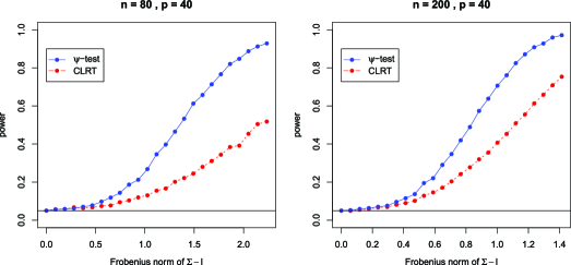
Figure 1: Power curves of the $\psi$ test (solid) and the CLRT (dashed) under the equi-correlation alternative. Each dot is obtained from $5000$ repetitions, and the curves are then obtained via linear interpolation.

4 Numerical experiments

In this section, a small simulation study is carried out to compare the power of the test $\psi$ defined in (10) with that of the CLRT under two specific alternatives.

The first alternative is the equi-correlation matrix $\Sigma=(\sigma_{ij})$, where for $\rho\in(0,1)$,

$$\sigma_{ij}=\cases{1,&\quad$i=j$,\cr\rho,&\quad$i\neq j$.}$$

Figure 1 shows how the power functions of the $\psi$ test and the CLRT grow with $\|\Sigma-I\|_{F}$ when $p=40$ and $n=80$ or $200$. For both tests, the significance levels are fixed at $\alpha=0.05$. To make a fair comparison, the $95$th percentiles of the null distributions of both test statistics are obtained via simulation instead of using those of the asymptotic normal distributions. From Figure 1, it is clear that the $\psi$ test is more powerful than the CLRT for both $(n,p)$ configurations. The difference between the powers is smaller when $n/p$ is larger. This is not surprising, because the LRT is a powerful test in the “large $n$, small $p$” regime.

The second alternative is the tridiagonal matrix $\Sigma=(\sigma_{ij})$, where for $\rho\in(0,1)$,

$$\sigma_{ij}=\cases{1,&\quad$i=j$,\cr\rho,&\quad$|i-j|=1$,\cr 0,&\quad$|i-j|>1$.}$$

Figure 2 shows how the power functions of the $\psi$ test and the CLRT grow with $\|\Sigma-I\|_{F}$ for the tridiagonal alternative. All the other setups remain unchanged. Here, the power of the $\psi$ test still dominates, while the difference in power between the two tests is smaller.

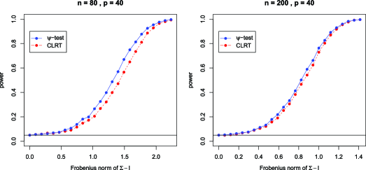
Figure 2: Power curves of the $\psi$ test (solid) and the CLRT (dashed) against the tridiagonal alternative. Each dot is obtained from $5000$ repetitions, and the curves are then obtained via linear interpolation.

5 Discussion

We have focused in the present paper on testing the hypotheses under the Frobenius norm. The technical arguments developed in this paper can also be used for testing under other matrix norms. Consider, for example, testing (1) against the following composite alternative hypothesis

$$H_{1}\colon\ \Sigma\in\Theta,\qquad\mbox{where }\Theta=\Theta_{n}=\bigl{\{}\|\Sigma-I\|_{s}\geq\varepsilon_{n}\bigr{\}}.$$

Here $\|A\|_{s}$ is the spectral norm defined by $\|A\|_{s}=\max_{\|x\|_{2}=1}\|Ax\|_{2}$. Define

$$\Theta_{s}(b)=\bigl{\{}\Sigma\colon\ \|\Sigma-I\|_{s}\geq b\sqrt{p/n}\bigr{\}}.$$ (16)

Then the same lower bound holds for $\Theta_{s}(b)$. To be more precise, we have the following result.

Theorem 6

Let $0<\alpha<\beta<1$. Suppose that as $n\to\infty$, $p\to\infty$ and $p/n\leq\kappa$ for some constant $\kappa<\infty$ and all $n$. Then there exist a constant $b=b(\kappa,\beta-\alpha)<1$, such that for any test $\phi$ with significance level $0<\alpha<1$ for testing $H_{0}\colon\ \Sigma=I$,

$$\limsup_{n\to\infty}\inf_{\Sigma\in\Theta_{s}(b)}\mathsf{E}_{\Sigma}\phi<\beta.$$

The proof of Theorem 6 is analogous to that of Theorem 1. We believe that the rate of $\sqrt{p/n}$ in the lower bound is sharp. It is however unclear which test is optimal against the alternative (16) under the spectral norm. Obtaining a matching upper bound for a practically useful test is an interesting project for future research.

The results in the current paper also shed light on the problem of testing for independence, that is, $H_{0}\colon\ R=I$, where $R$ is the population correlation matrix. Following Remark 1, the proof of Theorems 1 and 6 can be used directly to establish the same lower bound results on testing the correlation matrix.

Onatski et al. [15] also studied the hypothesis testing problem (1), but their attention is restricted to testing against alternatives that are rank one perturbations to the identity matrix. That is, under the alternative $H_{1}$ the covariance matrix belongs to the set $\Theta_{h}=\{I+hvv^{\prime}\colon\ \|v\|_{2}=1\}$. The asymptotic regime is restricted to $p/n\to c\in(0,\infty)$. In this asymptotic regime, Theorem 7 in [15] gives a lower bound result analogous to Theorem 1. However, it does not cover the case when $p/n\to 0$, nor can it be extended to the case of testing correlation matrices. In addition, we notice that though the result in [15] enables one to study the asymptotic power of all the eigenvalue-based tests on each $\Theta_{h}$ when $p/n\to c\in(0,\infty)$, it does not give a minimax claim as we did in Theorem 4.

The results in this paper also raised a number of interesting questions for future research. One example is the testing of equality of two covariance matrices based on the independent random samples $X_{1},\dots,X_{n_{1}}\stackrel{{\scriptstyle\mathrm{i.i.d.}}}{{\sim}}N_{p}(\mu_{1},\Sigma_{1})$ and $Y_{1},\dots,Y_{n_{2}}\stackrel{{\scriptstyle\mathrm{i.i.d.}}}{{\sim}}N_{p}(\mu_{2},\Sigma_{2})$. The validity of many commonly used statistical procedures including the classical Fisher’s linear discriminant analysis requires the assumption of equal covariance matrices. So it is of interest to test $H_{0}\colon\ \Sigma_{1}=\Sigma_{2}$. Motivated by an unbiased estimator of the Frobenius norm of $\Sigma_{1}-\Sigma_{2}$, Chen and Li [6] proposed a test using a linear combination of $U$-statistics and studied its power. Cai et al. [5] introduced a test based on the maximum of the standardized differences between the entries of the two sample covariance matrices. The test is shown to be powerful against sparse alternatives and robust with respect to the population distributions. However, the optimality of the two-sample tests has not been well studied. This is an important topic for future research that is of both theoretical and practical interest.

In the present paper, no structural assumption is imposed on the alternative class of the covariance matrices such as sparsity or bandedness. An optimal test against a structured alternative is potentially very different from the test (10) considered here. Recently, Cai and Jiang [4] considered testing the null hypothesis that $\Sigma$ is a banded matrix and introduced a test based on the coherence of a random matrix. Xiao and Wu [18] proposed a test for testing $H_{0}\colon\ \Sigma=I$ against sparse alternatives. Their test is based on the maximum of the standardized entries of the sample covariance matrix. The limiting null distribution is shown to be a type I extreme value distribution, the power of the test is not analyzed. It is interesting to investigate the optimality of these testing problems with structured alternatives.

6 Proofs

In this section, we prove Theorems 1, 4 and Propositions 3 and 5.

6.1 Proof of Theorem 1

Recall that $P_{0}$ is the probability measure when $X_{1},\dots X_{n}\stackrel{{\scriptstyle\mathrm{i.i.d.}}}{{\sim}}N_{p}(0,I)$ and $P_{v}$ is the probability measure when $X_{1},\dots,X_{n}\stackrel{{\scriptstyle\mathrm{i.i.d.}}}{{\sim}}N_{p}(0,\Sigma_{v})$. In addition, $P_{1}=\frac{1}{2^{p}}\sum_{v\in\{\pm 1\}^{p}}P_{v}$ is the average measure of the $P_{v}$’s. Let $f_{0}$ and $f_{1}$ be the density functions of $P_{0}$ and $P_{1}$, respectively. By the discussion following Theorem 1, we could prove Theorem 1 by showing that $\int f_{1}^{2}/f_{0}-1\leq 4(\beta-\alpha)^{2}$.

After some basic calculation (see Appendix A.1 for details), we obtain that if $b<b_{0}(\kappa)$ such that

$$b<1\quad\mbox{and}\quad\frac{bp}{\sqrt{n(p-1)}}<\frac{1}{\sqrt{2}},$$ (17)

then

$$\int\frac{f_{1}^{2}}{f_{0}}=\frac{(1-a^{2})^{n-np/2}}{[1+(p-1)a^{2}]^{n}}\mathsf{E}\biggl{[}1-\biggl{(}\frac{pa}{1+(p-1)a^{2}}\biggr{)}^{2}\biggl{(}\frac{\mathbf{1}^{\prime}V}{p}\biggr{)}^{2}\biggr{]}^{-n/2}.$$ (18)

Here, the expectation is taken w.r.t. $V=(V_{1},\dots,V_{p})^{\prime}$ where the $V_{j}$’s are i.i.d. Rademacher random variables which take values $\pm 1$ with equal probability.

Note that (17) and $p/n\leq\kappa$ implies

$$\biggl{(}\frac{pa}{1+(p-1)a^{2}}\biggr{)}^{2}\leq\frac{1}{2}.$$

Also note that $(\mathbf{1}^{\prime}V/p)^{2}\in[0,1]$. Thus, let $\tilde{b}_{np}=(\frac{pa}{1+(p-1)a^{2}})^{2}$, and $(\mathbf{1}^{\prime}V/p)^{2}=\xi_{p}$, we have

$$\mathsf{E}(1-\tilde{b}_{np}\xi_{p})^{-n/2} = \mathsf{E}\bigl{[}(1-\tilde{b}_{np}\xi_{p})^{-1/(\tilde{b}_{np}\xi_{p})}\bigr{]}^{n\tilde{b}_{np}\xi_{p}/2}$$

$$\leq \mathsf{E}\exp\biggl{(}\frac{\log{4}}{2}n\tilde{b}_{np}\xi_{p}\biggr{)}\qquad\bigl{(}0\leq(1-x)^{1/x}\leq 4,\mbox{ for all }x\in[0,1/2]\bigr{)}$$

$$\leq \mathsf{E}\exp\biggl{(}\frac{\log{4}}{2}\frac{b^{2}p^{2}}{p-1}\xi_{p}\biggr{)}\qquad\bigl{(}\tilde{b}_{np}\leq p^{2}b^{2}/\bigl{[}n(p-1)\bigr{]}\bigr{)}.$$

For $\xi_{p}$, Hoeffding’s inequality [9], applied to Rademacher variables, yields

$$\mathsf{P}(\xi_{p}\geq\lambda)\leq 2\mathrm{e}^{-2p\lambda}\qquad\mbox{for all }\lambda>0.$$

Thus, we obtain

$$\mathsf{E}\exp\biggl{(}\frac{\log{4}}{2}\frac{b^{2}p^{2}}{p-1}\xi_{p}\biggr{)} = \int_{0}^{\infty}\mathsf{P}\biggl{(}\exp\biggl{(}\frac{\log{4}}{2}\frac{b^{2}p^{2}}{p-1}\xi_{p}\biggr{)}\geq u\biggr{)}\,\mathrm{d}u$$

$$= 1+\int_{1}^{\infty}\mathsf{P}\biggl{(}\xi_{p}\geq\frac{2\log u}{\log 4}\frac{p-1}{b^{2}p^{2}}\biggr{)}\,\mathrm{d}u$$

$$\leq 1+\int_{1}^{\infty}2\exp\biggl{(}-\frac{4(p-1)\log{u}}{b^{2}p\log 4}\biggr{)}\,\mathrm{d}u$$

$$= 1+\frac{2b^{2}p\log{2}}{2(p-1)-b^{2}p\log{2}}.$$

Here, the last equality holds if $2(p-1)>b^{2}p\log{2}$, which is always true for large $p$ since $b<1$.

In addition, with $b$ satisfying (17), when $n\to\infty$,

$$\bigl{(}1-a^{2}\bigr{)}^{n-np/2}\to\mathrm{e}^{b^{2}},\qquad\bigl{[}1+(p-1)a^{2}\bigr{]}^{n}\to\mathrm{e}^{b^{2}}.$$

Therefore, for large enough $n\geq n_{0}(\kappa)$,

$$\int\frac{f_{1}^{2}}{f_{0}}-1\leq\frac{8b^{2}p\log{2}}{2(p-1)-b^{2}p\log{2}},$$

which, for sufficiently small $b\leq b_{0}(\kappa,\beta-\alpha)$, is no larger than $4(\beta-\alpha)^{2}$. This completes the proof.

6.2 Proof of Proposition 3

Following the outline of proof after Proposition 3, for $E_{1}$ and $E_{2}$ defined in (14), we complete the proof below by showing that $E_{1}/\sigma^{4}_{n}(\Sigma)=\mathrm{O}(1/n)$ and $E_{2}/\sigma^{4}_{n}(\Sigma)=\mathrm{O}(\operatorname{tr}(\Sigma^{4})/\operatorname{tr}^{2}(\Sigma^{2}))$.

To this end, we start with some preliminaries. Throughout the proof, $\mathsf{E}$ and $\operatorname{\mathsf{Var}}$ are used as abbreviations for $\mathsf{E}_{\Sigma}$ and $\operatorname{\mathsf{Var}}_{\Sigma}$, respectively. Recall the martingale representation (11), where each martingale difference $D_{nk}$ has the explicit expression (3.2). For $D_{nk}$, its conditional variance is

$$\sigma_{nk}^{2} = \mathsf{E}_{k-1}\bigl{[}D_{nk}^{2}\bigr{]}$$

$$= \frac{8}{n^{2}(n-1)^{2}}\operatorname{tr}(Q_{k-1}\Sigma Q_{k-1}\Sigma)+\frac{16}{n^{2}(n-1)}\operatorname{tr}\bigl{(}Q_{k-1}\Sigma^{3}\bigr{)}$$

$${}-\frac{16}{n^{2}(n-1)}\operatorname{tr}\bigl{(}Q_{k-1}\Sigma^{2}\bigr{)}+\frac{8}{n^{2}}\operatorname{tr}\bigl{(}\Sigma^{2}(\Sigma-I)^{2}\bigr{)}.$$

Detailed derivation of (3.2) and (6.2) can be found in Appendix A.3. With (6.2), it is not difficult to verify that

$$\mathsf{E}\bigl{[}\sigma_{nk}^{2}\bigr{]}=\frac{8(k-1)}{n^{2}(n-1)^{2}}\bigl{[}\operatorname{tr}^{2}\bigl{(}\Sigma^{2}\bigr{)}+\operatorname{tr}\bigl{(}\Sigma^{4}\bigr{)}\bigr{]}+\frac{8}{n^{2}}\operatorname{tr}\bigl{(}\Sigma^{2}(\Sigma-I)^{2}\bigr{)},$$

and that $\sigma_{n}^{2}=\operatorname{\mathsf{Var}}(T_{n})=\sum_{k=1}^{n}\mathsf{E}[\sigma_{nk}^{2}]$. Last but not least, we have for any $j>k$,

$$\mathsf{E}_{k-1}\bigl{[}\sigma_{nj}^{2}-\mathsf{E}\sigma_{nj}^{2}\bigr{]}=\sigma_{nk}^{2}-\mathsf{E}\sigma_{nk}^{2}.$$ (20)

Now, we turn to the studies of $E_{1}$ and $E_{2}$.

Term $E_{1}$. We begin with the first term. Decompose the covariance matrix (as in [7]) as $\Sigma=\Gamma\Gamma^{\prime}$, with $\Gamma\in\mathbb{R}^{p\times p}$. Then, we have the representation

$$X_{i}=\Gamma Z_{i},\qquad Z_{i}\stackrel{{\scriptstyle\mathrm{i.i.d.}}}{{\sim}}N_{p}(0,I),\qquad i=1,\dots,n.$$ (21)

We further define

$$A=\Gamma^{\prime}\Gamma,\qquad M_{k-1}=\Gamma^{\prime}\sum_{i=1}^{k-1}\bigl{(}X_{i}X_{i}^{\prime}-\Sigma\bigr{)}\Gamma=A\sum_{i=1}^{k-1}\bigl{(}Z_{i}Z_{i}^{\prime}-I\bigr{)}A.$$

With the above definition, (3.2) can be rewritten as

$$D_{nk}=\frac{2}{n(n-1)}\bigl{[}Z_{k}^{\prime}M_{k-1}Z_{k}-\operatorname{tr}(M_{k-1})\bigr{]}+\frac{2}{n}\bigl{[}Z_{k}^{\prime}\bigl{(}A^{2}-A\bigr{)}Z_{k}-\operatorname{tr}\bigl{(}A^{2}-A\bigr{)}\bigr{]}.$$

Therefore, we obtain from the Cauchy–Schwarz inequality and Lemma 3 that

$$\mathsf{E}\bigl{[}D_{nk}^{4}\bigr{]} \leq \frac{C}{n^{4}}\mathsf{E}\bigl{[}Z_{k}^{\prime}\bigl{(}A^{2}-A\bigr{)}Z_{k}-\operatorname{tr}\bigl{(}A^{2}-A\bigr{)}\bigr{]}^{4}+\frac{C}{n^{4}(n-1)^{4}}\mathsf{E}\bigl{[}Z_{k}^{\prime}M_{k-1}Z_{k}-\operatorname{tr}(M_{k-1})\bigr{]}^{4}$$

$$\leq \frac{C}{n^{4}}\operatorname{tr}^{2}\bigl{(}\Sigma^{2}(\Sigma-I)^{2}\bigr{)}+\frac{C}{n^{4}(n-1)^{4}}\mathsf{E}\bigl{[}\operatorname{tr}^{2}\bigl{(}M_{k-1}^{2}\bigr{)}\bigr{]}.$$

For $\operatorname{tr}(M_{k-1}^{2})$, we use the following lemma, the proof of which is given in Appendix A.3.

Lemma 2

For $\operatorname{tr}(M_{k-1}^{2})$, we have

$$\mathsf{E}\bigl{[}\operatorname{tr}\bigl{(}M_{k-1}^{2}\bigr{)}\bigr{]} = (k-1)\bigl{[}\operatorname{tr}^{2}\bigl{(}\Sigma^{2}\bigr{)}+\operatorname{tr}\bigl{(}\Sigma^{4}\bigr{)}\bigr{]},$$

$$\operatorname{\mathsf{Var}}\bigl{[}\operatorname{tr}\bigl{(}M_{k-1}^{2}\bigr{)}\bigr{]} = (k-1)\bigl{[}24\operatorname{tr}\bigl{(}\Sigma^{8}\bigr{)}+16\operatorname{tr}\bigl{(}\Sigma^{6}\bigr{)}\operatorname{tr}\bigl{(}\Sigma^{2}\bigr{)}+8\operatorname{tr}^{2}\bigl{(}\Sigma^{4}\bigr{)}+8\operatorname{tr}\bigl{(}\Sigma^{4}\bigr{)}\operatorname{tr}^{2}\bigl{(}\Sigma^{2}\bigr{)}\bigr{]}$$

$${}+2(k-1)(k-2)\bigl{[}6\operatorname{tr}\bigl{(}\Sigma^{8}\bigr{)}+2\operatorname{tr}^{2}\bigl{(}\Sigma^{4}\bigr{)}\bigr{]}.$$

For any sequences $\{a_{n}\}$ and $\{b_{n}\}$ of positive numbers, write $a_{n}\lesssim b_{n}$ if $\limsup_{n\to\infty}a_{n}/\break b_{n}<\infty$. Note that $\operatorname{tr}(\Sigma^{6})\leq\operatorname{tr}(\Sigma^{4})\operatorname{tr}(\Sigma^{2})$ and $\operatorname{tr}(\Sigma^{8})\leq\operatorname{tr}^{2}(\Sigma^{4})$. Since $\operatorname{tr}(\Sigma^{4})=\mathrm{o}(\operatorname{tr}^{2}(\Sigma^{2}))$, Lemma 2 implies that

$$\mathsf{E}\bigl{[}D_{nk}^{4}\bigr{]}\lesssim\frac{1}{n^{4}}\operatorname{tr}^{2}\bigl{(}\Sigma^{2}(\Sigma-I)^{2}\bigr{)}+\frac{k^{2}}{n^{8}}\operatorname{tr}^{4}\bigl{(}\Sigma^{2}\bigr{)},$$

and hence

$$E_{1}\lesssim\frac{1}{n^{3}}\operatorname{tr}^{2}\bigl{(}\Sigma^{2}(\Sigma-I)^{2}\bigr{)}+\frac{1}{n^{5}}\operatorname{tr}^{4}\bigl{(}\Sigma^{2}\bigr{)}.$$ (22)

Term $E_{2}$. For $E_{2}$, we can simplify it as

$$E_{2} = \mathsf{E}\Biggl{[}\sum_{k=1}^{n}\bigl{(}\sigma_{nk}^{2}-\mathsf{E}\sigma_{nk}^{2}\bigr{)}\Biggr{]}^{2}$$

$$= \mathsf{E}\Biggl{[}\sum_{k=1}^{n}\bigl{(}\sigma_{nk}^{2}-\mathsf{E}\sigma_{nk}^{2}\bigr{)}^{2}+2\sum_{k=1}^{n-1}\sum_{l=k+1}^{n}\bigl{(}\sigma_{nk}^{2}-\mathsf{E}\sigma_{nk}^{2}\bigr{)}\bigl{(}\sigma_{nl}^{2}-\mathsf{E}\sigma_{nl}^{2}\bigr{)}\Biggr{]}$$

$$= \sum_{k=1}^{n}\operatorname{\mathsf{Var}}\bigl{(}\sigma_{nk}^{2}\bigr{)}+2\sum_{k=1}^{n-1}(n-k)\operatorname{\mathsf{Var}}\bigl{(}\sigma_{nk}^{2}\bigr{)}=\sum_{k=1}^{n}(2n-2k+1)\operatorname{\mathsf{Var}}\bigl{(}\sigma_{nk}^{2}\bigr{)}.$$

Here, the second equality comes from (20).

Note that $\operatorname{tr}(Q_{k-1}\Sigma Q_{k-1}\Sigma)=\operatorname{tr}(M_{k-1}^{2})$ and $\operatorname{tr}(Q_{k-1}(\Sigma^{3}-\Sigma^{2}))=\operatorname{tr}(M_{k-1}(A^{2}-A))$. So, by (6.2), there exist numeric constants $C$ and $C^{\prime}$, such that

$$\operatorname{\mathsf{Var}}\bigl{(}\sigma_{nk}^{2}\bigr{)}\leq\frac{C}{n^{4}(n-1)^{4}}\operatorname{\mathsf{Var}}\bigl{[}\operatorname{tr}\bigl{(}M_{k-1}^{2}\bigr{)}\bigr{]}+\frac{C^{\prime}}{n^{4}(n-1)^{2}}\operatorname{\mathsf{Var}}\bigl{[}\operatorname{tr}\bigl{(}M_{k-1}\bigl{(}A^{2}-A\bigr{)}\bigr{)}\bigr{]}.$$

We have studied $\operatorname{\mathsf{Var}}[\operatorname{tr}(M_{k-1}^{2})]$ in Lemma 2. On the other hand, we have from Lemma 3 that

$$\operatorname{\mathsf{Var}}\bigl{[}\operatorname{tr}\bigl{(}M_{k-1}\bigl{(}A^{2}-A\bigr{)}\bigr{)}\bigr{]} = (k-1)\operatorname{\mathsf{Var}}\bigl{[}\operatorname{tr}\bigl{(}AZZ^{\prime}A\bigl{(}A^{2}-A\bigr{)}\bigr{)}\bigr{]}=(k-1)\operatorname{\mathsf{Var}}\bigl{[}Z^{\prime}\bigl{(}A^{4}-A^{3}\bigr{)}Z\bigr{]}$$

$$= (k-1)\bigl{\{}\mathsf{E}\bigl{[}\bigl{(}Z^{\prime}\bigl{(}A^{4}-A^{3}\bigr{)}Z\bigr{)}^{2}\bigr{]}-\bigl{[}\mathsf{E}\bigl{[}Z^{\prime}\bigl{(}A^{4}-A^{3}\bigr{)}Z\bigr{]}\bigr{]}^{2}\bigr{\}}$$

$$= (k-1)\bigl{[}2\operatorname{tr}\bigl{(}\bigl{(}A^{4}-A^{3}\bigr{)}^{2}\bigr{)}+\operatorname{tr}^{2}\bigl{(}A^{4}-A^{3}\bigr{)}-\operatorname{tr}^{2}\bigl{(}A^{4}-A^{3}\bigr{)}\bigr{]}$$

$$= 2(k-1)\operatorname{tr}\bigl{(}\Sigma^{6}(\Sigma-I)^{2}\bigr{)}$$

$$\leq 2(k-1)\operatorname{tr}\bigl{(}\Sigma^{4}\bigr{)}\operatorname{tr}\bigl{(}\Sigma^{2}(\Sigma-I)^{2}\bigr{)}.$$

Since $\operatorname{tr}(\Sigma^{6})\leq\operatorname{tr}(\Sigma^{4})\operatorname{tr}(\Sigma^{2})$, $\operatorname{tr}(\Sigma^{8})\leq\operatorname{tr}^{2}(\Sigma^{4})$ and $\operatorname{tr}(\Sigma^{4})=\mathrm{o}(\operatorname{tr}^{2}(\Sigma^{2}))$, we obtain that

$$\operatorname{\mathsf{Var}}\bigl{(}\sigma_{nk}^{2}\bigr{)}\lesssim\frac{k}{n^{8}}\operatorname{tr}\bigl{(}\Sigma^{4}\bigr{)}\operatorname{tr}^{2}\bigl{(}\Sigma^{2}\bigr{)}+\frac{k^{2}}{n^{2}}\operatorname{tr}^{2}\bigl{(}\Sigma^{4}\bigr{)}+\frac{k}{n^{6}}\operatorname{tr}\bigl{(}\Sigma^{4}\bigr{)}\operatorname{tr}\bigl{(}\Sigma^{2}(\Sigma-I)^{2}\bigr{)},$$

which leads to the bound

$$E_{2}\lesssim\frac{1}{n^{3}}\operatorname{tr}\bigl{(}\Sigma^{4}\bigr{)}\operatorname{tr}\bigl{(}\Sigma^{2}(\Sigma-I)^{2}\bigr{)}+\frac{1}{n^{4}}\operatorname{tr}^{2}\bigl{(}\Sigma^{4}\bigr{)}+\frac{1}{n^{5}}\operatorname{tr}\bigl{(}\Sigma^{4}\bigr{)}\operatorname{tr}^{2}\bigl{(}\Sigma^{2}\bigr{)}.$$ (23)

Summing up. By (9), we have

$$\sigma_{n}^{4}\asymp\frac{1}{n^{2}}\operatorname{tr}^{2}\bigl{(}\Sigma^{2}(\Sigma-I)^{2}\bigr{)}+\frac{1}{n^{3}}\operatorname{tr}^{2}\bigl{(}\Sigma^{2}\bigr{)}\operatorname{tr}\bigl{(}\Sigma^{2}(\Sigma-I)^{2}\bigr{)}+\frac{1}{n^{4}}\operatorname{tr}^{4}\bigl{(}\Sigma^{2}\bigr{)}.$$ (24)

Here and after, for any sequences $\{a_{n}\}$ and $\{b_{n}\}$ of positive numbers, we write $a_{n}\asymp b_{n}$ if $a_{n}/b_{n}$ is bounded away from both $0$ and $\infty$. Thus, we obtain that

$$\sigma_{n}^{-4}E_{1}=\mathrm{O}\bigl{(}n^{-1}\bigr{)},\qquad\sigma_{n}^{-4}E_{2}=\mathrm{O}\bigl{(}\operatorname{tr}\bigl{(}\Sigma^{4}\bigr{)}/\operatorname{tr}^{2}\bigl{(}\Sigma^{2}\bigr{)}\bigr{)}.$$

Plugging these estimates in Lemma 1, we complete the proof.

6.3 Proof of Theorem 4

Following the discussion after Theorem 4, we give below the detailed proof of the first claim in the theorem. In particular, we bound the power of the test separately on $\Theta(B)$ and $\Theta(b,B)$, which are defined in (3.3).

Case 1: $\Theta(B)$. Here, we shall proceed heavy-handedly by using Chebyshev’s inequality, because the alternative class is sufficiently far away from $H_{0}$.

For any $\Sigma\in\Theta(B)$, there exists $\tau\geq B$, s.t. $\|\Sigma-I\|_{F}=\tau\sqrt{p/n}$. Suppose $B$ is large enough s.t. $\tau^{2}\geq B^{2}\geq 3z_{1-\alpha}$. Note that $\sigma_{n}(I)=(2p/n)(1+\mathrm{o}(1))$, and so

$$\mathsf{E}_{\Sigma}T_{n}=\|\Sigma-I\|_{F}^{2}=\frac{\tau^{2}}{2}\sigma_{n}(I)\bigl{(}1+\mathrm{o}(1)\bigr{)}>z_{1-\alpha}\sigma_{n}(I).$$

Thus, we can use Chebyshev’s inequality to bound the type II error of $\psi$ at $\Sigma$ as the following:

$$1-\mathsf{E}_{\Sigma}\psi = \mathsf{P}_{\Sigma}\bigl{(}T_{n}\leq z_{1-\alpha}\sigma_{n}(I)\bigr{)}=\mathsf{P}_{\Sigma}\bigl{(}T_{n}-\mathsf{E}_{\Sigma}T_{n}\leq z_{1-\alpha}\sigma_{n}(I)-\mathsf{E}_{\Sigma}T_{n}\bigr{)}$$

$$\leq \mathsf{P}_{\Sigma}\bigl{(}|T_{n}-\mathsf{E}_{\Sigma}T_{n}|\geq|z_{1-\alpha}\sigma_{n}(I)-\mathsf{E}_{\Sigma}T_{n}|\bigr{)}$$

$$\leq \frac{\operatorname{\mathsf{Var}}_{\Sigma}(T_{n})}{[z_{1-\alpha}\sigma_{n}(I)-\mathsf{E}_{\Sigma}T_{n}]^{2}}.$$

For $\operatorname{\mathsf{Var}}_{\Sigma}(T_{n})=\sigma_{n}^{2}(\Sigma)$, we have its explicit expression given in (9). Let $\lambda_{\max}(\Sigma)$ denote the largest eigenvalue of $\Sigma$. When $\|\Sigma-I\|_{F}=\tau\sqrt{p/n}$, we have $\lambda_{\max}(\Sigma)\leq 1+\tau\sqrt{p/n}$, and so

$$\operatorname{tr}\bigl{(}\Sigma^{2}\bigr{)}\leq p\biggl{(}1+\frac{\tau}{\sqrt{n}}\biggr{)}^{2},\qquad\operatorname{tr}\bigl{(}\Sigma^{2}(\Sigma-I)^{2}\bigr{)}\leq\lambda_{\max}^{2}(\Sigma)\|\Sigma-I\|_{F}^{2}\leq\frac{\tau^{2}p}{n}\biggl{(}1+\tau\sqrt{\frac{p}{n}}\biggr{)}^{2}.$$

Since $\operatorname{tr}(\Sigma^{4})\leq\operatorname{tr}^{2}(\Sigma^{2})$ and $\sigma_{n}^{2}(I)=(4p^{2}/n^{2})(1+\mathrm{o}(1))$, the above inequalities, together with (9), lead to

$$\frac{\sigma_{n}^{2}(\Sigma)}{\sigma_{n}^{2}(I)}\leq\biggl{[}2\biggl{(}1+\frac{\tau}{\sqrt{n}}\biggr{)}^{2}+\frac{2\tau^{2}}{p}\biggl{(}1+\tau\sqrt{\frac{p}{n}}\biggr{)}^{2}\biggr{]}\bigl{(}1+\mathrm{o}(1)\bigr{)}.$$

Since $\tau^{2}/2-z_{1-\alpha}\geq\tau^{2}/6$ , there exists some constant $C_{\alpha}$ depending only on $\alpha$, such that

$$\frac{\operatorname{\mathsf{Var}}_{\Sigma}(T_{n})}{[z_{1-\alpha}\sigma_{n}(I)-\mathsf{E}_{\Sigma}T_{n}]^{2}} \leq \frac{2(1+{\tau}/{\sqrt{n}})^{2}+({2\tau^{2}}/{p})(1+\tau\sqrt{{p}/{n}})^{2}}{(\tau^{2}/2-z_{1-\alpha})^{2}}\bigl{(}1+\mathrm{o}(1)\bigr{)}$$

$$\leq C_{\alpha}\biggl{[}\biggl{(}\frac{1}{\sqrt{\tau}}+\frac{1}{\sqrt{n}}\biggr{)}^{4}+\frac{1}{\tau^{2}p}+\frac{1}{n}\biggr{]}.$$

Note that all the $\mathrm{o}(1)$ terms in the above derivation are uniform over $\Theta(B)$. Therefore, given $\alpha$ and $b$, there exist a constant $B=B(\alpha,b)$, such that

$$\liminf_{n\to\infty}\inf_{\Theta(B)}\mathsf{E}_{\Sigma}\psi \geq 1-\frac{\operatorname{\mathsf{Var}}_{\Sigma}(T_{n})}{[z_{1-\alpha}\sigma_{n}(I)-\mathsf{E}_{\Sigma}T_{n}]^{2}}$$

$$\geq 1-C_{\alpha}\biggl{[}\biggl{(}\frac{1}{\sqrt{B}}+\frac{1}{\sqrt{n}}\biggr{)}^{4}+\frac{1}{B^{2}p}+\frac{1}{n}\biggr{]}$$

$$\geq 1-\Phi\biggl{(}z_{1-\alpha}-\frac{b^{2}}{2}\biggr{)}>\alpha.$$

Case 2: $\Theta(b,B)$. On this subset, we use Proposition 3 to obtain the following uniform approximation to the power function by the normal distribution function

$$\sup_{\Theta(b,B)}\biggl{|}\mathsf{E}_{\Sigma}\psi-\Phi\biggl{(}z_{1-\alpha}-\frac{\|\Sigma-I\|_{F}^{2}}{2p/n}\biggr{)}\biggr{|}\to 0.$$ (27)

If (27) is true, then we obtain

$$\lim_{n\to\infty}\inf_{\Theta(b,B)}\mathsf{E}_{\Sigma}\psi=\lim_{n\to\infty}\inf_{\Theta(b,B)}\Phi\biggl{(}z_{1-\alpha}-\frac{\|\Sigma-I\|_{F}^{2}}{2p/n}\biggr{)}=1-\Phi\biggl{(}z_{1-\alpha}-\frac{b^{2}}{2}\biggr{)}>\alpha.$$

Together with (6.3), this leads to the desired claim.

Turn to the proof of (27). First, note that uniformly on $\Theta(b,B)$, we have

$$p(1-B/\sqrt{n})^{2}\leq\operatorname{tr}\bigl{(}\Sigma^{2}\bigr{)}\leq p(1+B/\sqrt{n})^{2},$$ (28)

and $\operatorname{tr}(\Sigma^{4})\leq\lambda_{\max}^{2}(\Sigma)\operatorname{tr}(\Sigma^{2})\leq B^{2}(p/n)p(1+B/\sqrt{n})^{2}$. Therefore, as $n\to\infty$,

$$\sup_{\Theta(b,B)}|\operatorname{tr}\bigl{(}\Sigma^{2}\bigr{)}/p-1|\to 0,\qquad\sup_{\Theta(b,B)}\operatorname{tr}\bigl{(}\Sigma^{4}\bigr{)}/\operatorname{tr}^{2}\bigl{(}\Sigma^{2}\bigr{)}\to 0.$$ (29)

So the condition of Proposition 3 is satisfied. Next, we observe that

$$\mathsf{E}_{\Sigma}\psi = \mathsf{P}_{\Sigma}\bigl{(}T_{n}>z_{1-\alpha}\sigma_{n}(I)\bigr{)}=\mathsf{P}_{\Sigma}\biggl{(}\frac{T_{n}-\|\Sigma-I\|_{F}^{2}}{\sigma_{n}(\Sigma)}\geq\frac{\sigma_{n}(I)}{\sigma_{n}(\Sigma)}z_{1-\alpha}-\frac{\|\Sigma-I\|_{F}^{2}}{\sigma_{n}(\Sigma)}\biggr{)}$$

$$= \mathsf{P}_{\Sigma}\biggl{(}\frac{T_{n}-\mu_{n}(\Sigma)}{\sigma_{n}(\Sigma)}\geq\frac{\sigma_{n}(I)}{\sigma_{n}(\Sigma)}z_{1-\alpha}-\frac{\|\Sigma-I\|_{F}^{2}}{\sigma_{n}(\Sigma)}\biggr{)}.$$

Thus, Proposition 3 and (29) together imply that

$$\sup_{\Theta(b,B)}\biggl{|}\mathsf{E}_{\Sigma}\psi-\Phi\biggl{(}\frac{\sigma_{n}(I)}{\sigma_{n}(\Sigma)}z_{1-\alpha}-\frac{\|\Sigma-I\|_{F}^{2}}{\sigma_{n}(\Sigma)}\biggr{)}\biggr{|}\to 0.$$

To complete the proof, what is left to be verified is that

$$\sup_{\Theta(b,B)}\biggl{|}\frac{\sigma_{n}^{2}(\Sigma)}{4p^{2}/n^{2}}-1\biggr{|}\to 0,$$ (30)

because it implies $\sup_{\Theta(b,B)}|\Phi(z_{1-\alpha}-\frac{\|\Sigma-I\|_{F}^{2}}{2p/n})-\Phi(\frac{\sigma_{n}(I)}{\sigma_{n}(\Sigma)}z_{1-\alpha}-\frac{\|\Sigma-I\|_{F}^{2}}{\sigma_{n}(\Sigma)})|\to 0$, which together with the last display before (30), leads to (27). To show (30), first recall the expression of $\sigma_{n}^{2}(\Sigma)$ in (9). By (29), we obtain that the first term in (9) is $4(p^{2}/n^{2})(1+\mathrm{o}(1))$ where $\mathrm{o}(1)$ is uniform on $\Theta(b,B)$. On the other hand,

$$\operatorname{tr}\bigl{(}\Sigma^{2}(\Sigma-I)^{2}\bigr{)} \leq \lambda^{2}_{\max}(\Sigma)\|\Sigma-I\|_{F}^{2}$$

$$\leq \biggl{(}1+B\sqrt{\frac{p}{n}}\biggr{)}^{2}\frac{Bp}{n}\leq C(B)\max\biggl{(}1,\frac{p}{n}\biggr{)}\cdot\frac{p}{n}.$$

Here, $C(B)$ is a constant depending only on $B$. Therefore, we have that the second term in (9) is of order $\mathrm{o}(p^{2}/n^{2})$ uniformly over $\Theta(b,B)$. Putting the two parts together leads to (30). This completes the proof.

6.4 Proof of Proposition 5

Fix any $\tau\in(0,1)$. At each dimension $p$, consider a single point in $\mathbb{C}(\tau)$:

$$\Sigma^{*}=I_{p\times p}+\tau\sqrt{\frac{p}{n}}uu^{\prime},$$

where $u$ is an arbitrarily fixed unit vector in $\mathbb{R}^{p}$. Since $\tau<1$, Proposition 10 in [15] leads to

$$\lim_{n\to\infty}\mathsf{E}_{\Sigma^{*}}\phi_{\mathrm{CLR}}=1-\Phi\bigl{(}z_{1-\alpha}-h(\tau,c)\bigr{)}\qquad\mbox{for }h(\tau,c)=\frac{\tau\sqrt{c}-\log(1+\tau\sqrt{c})}{\sqrt{-2\log(1-c)-2c}}.$$

Note that for all $\tau>0$ and $c\in(0,1)$, $\tau^{2}/2>h(\tau,c)>0$. Therefore,

$$\lim_{n\to\infty}\inf_{\mathbb{C}(\tau)}\mathsf{E}_{\Sigma}\psi = 1-\Phi\biggl{(}z_{1-\alpha}-\frac{\tau^{2}}{2}\biggr{)}$$

$$> 1-\Phi\bigl{(}z_{1-\alpha}-h(\tau,c)\bigr{)}$$

$$= \lim_{n\to\infty}\mathsf{E}_{\Sigma^{*}}\phi_{\mathrm{CLR}}$$

$$\geq \limsup_{n\to\infty}\inf_{\mathbb{C}(\tau)}\mathsf{E}_{\Sigma}\phi_{\mathrm{CLR}}.$$

The proof of the second claim is obtained by replacing $\mathbb{C}(\tau)$ with $\Theta(b)$ and $\tau$ with $b$ in the above arguments.

Appendix: Technical details

A.1 Proof details for Theorem 1

Here we give the calculation leading to (18) in the proof of Theorem 1.

Consider $\Theta^{*}(b)$ in (5). For any $v\in\{\pm 1\}^{p}$, we have $\|\Sigma_{v}-I\|_{F}=b\sqrt{p/n}$, $\operatorname{diag}(\Sigma_{v})=(1,\dots,1)$, and for $a=b/\sqrt{n(p-1)}$,

$$\Sigma^{-1}_{v} = \frac{1}{1-a}I_{p\times p}-\biggl{[}\frac{1}{1-a}-\frac{1}{1+(p-1)a}\biggr{]}\frac{1}{p}vv^{\prime},$$

$$\det{\Sigma_{v}} = (1-a)^{p-1}\bigl{[}1+(p-1)a\bigr{]}.$$

Therefore, we have

$$f_{0}(x_{1},\dots,x_{n}) = \frac{1}{(2\uppi)^{np/2}}\exp\Biggl{\{}-\frac{1}{2}\sum_{i=1}^{n}x^{\prime}_{i}x_{i}\Biggr{\}},$$

$$f_{1}(x_{1},\dots,x_{n}) = \frac{1}{2^{p}}\sum_{v}\frac{1}{(2\uppi)^{np/2}(\det{\Sigma_{v}})^{n/2}}\exp\Biggl{\{}-\frac{1}{2}\sum_{i=1}^{n}x^{\prime}_{i}\Sigma_{v}^{-1}x_{i}\Biggr{\}}$$

$$= \frac{1}{(2\uppi)^{np/2}}\exp\Biggl{\{}-\frac{1}{2(1-a)}\sum_{i=1}^{n}x^{\prime}_{i}x_{i}\Biggr{\}}\frac{1}{(1-a)^{n(p-1)/2}[1+(p-1)a]^{n/2}}$$

$${}\times\frac{1}{2^{p}}\sum_{v}\exp\Biggl{\{}\frac{1}{2p}\biggl{[}\frac{1}{1-a}-\frac{1}{1+(p-1)a}\biggr{]}\sum_{i=1}^{n}\bigl{(}v^{\prime}x_{i}\bigr{)}^{2}\Biggr{\}}.$$

And so

$$\frac{f_{1}^{2}}{f_{0}} = \frac{1}{(1-a)^{n(p-1)}[1+a(p-1)]^{n}}\times\frac{1}{(2\uppi)^{np/2}}\exp\Biggl{\{}-\frac{1}{2}\biggl{(}\frac{1+a}{1-a}\biggr{)}\sum_{i=1}^{n}x^{\prime}_{i}x_{i}\Biggr{\}}$$

$${}\times\frac{1}{2^{2p}}\Biggl{\{}\sum_{v}\exp\Biggl{[}\frac{1}{p}\biggl{(}\frac{1}{1-a}-\frac{1}{1+(p-1)a}\biggr{)}\sum_{i=1}^{n}\bigl{(}v^{\prime}x_{i}\bigr{)}^{2}\Biggr{]}$$

$$\hskip 35.0pt{}+\sum_{v\neq u}\exp\Biggl{[}\frac{1}{2p}\biggl{(}\frac{1}{1-a}-\frac{1}{1+(p-1)a}\biggr{)}\Biggl{(}\sum_{{i=1}}^{n}\bigl{(}v^{\prime}x_{i}\bigr{)}^{2}+\sum_{1}^{n}\bigl{(}u^{\prime}x_{i}\bigr{)}^{2}\Biggr{)}\Biggr{]}\Biggr{\}}.$$

Now we compute the integral. Fix any $v$, we have

$$\int\frac{1}{(2\uppi)^{np/2}}\exp\Biggl{\{}-\frac{1}{2}\biggl{(}\frac{1+a}{1-a}\biggr{)}\sum_{i=1}^{n}x^{\prime}_{i}x_{i}\Biggr{\}}\exp\Biggl{\{}\frac{1}{p}\biggl{(}\frac{1}{1-a}-\frac{1}{1+(p-1)a}\biggr{)}\sum_{i=1}^{n}\bigl{(}v^{\prime}x_{i}\bigr{)}^{2}\Biggr{\}}\,\mathrm{d}x$$

$$\quad=\biggl{[}\int\frac{1}{(2\uppi)^{p/2}}\exp\biggl{\{}-\frac{1}{2}\biggl{(}\frac{1+a}{1-a}\biggr{)}x^{\prime}x\biggr{\}}\exp\biggl{\{}\frac{1}{p}\biggl{(}\frac{1}{1-a}-\frac{1}{1+(p-1)a}\biggr{)}\bigl{(}v^{\prime}x\bigr{)}^{2}\biggr{\}}\,\mathrm{d}x\biggr{]}^{n}$$

$$\quad=\biggl{(}\frac{1+a}{1-a}\biggr{)}^{-np/2}\bigl{[}\mathsf{E}\exp(tY)\bigr{]}^{n}$$

$$\quad=\biggl{(}\frac{1+a}{1-a}\biggr{)}^{-np/2}(1-2t)^{-n/2}\qquad\mbox{(for $t\leq 1/2$)},$$

where $Y\sim\chi^{2}_{(1)}$, and

$$t=\biggl{(}\frac{1}{1-a}-\frac{1}{1+(p-1)a}\biggr{)}\biggl{(}\frac{1+a}{1-a}\biggr{)}^{-1}.$$ (32)

In addition, fix any $v\neq u$, we have

$$\int\frac{1}{(2\uppi)^{np/2}}\exp\Biggl{\{}-\frac{1}{2}\biggl{(}\frac{1+a}{1-a}\biggr{)}\sum_{i=1}^{n}x^{\prime}_{i}x_{i}\Biggr{\}}$$

$$\qquad{}\times\exp\Biggl{\{}\frac{1}{2p}\biggl{(}\frac{1}{1-a}-\frac{1}{1+(p-1)a}\biggr{)}\Biggl{(}\sum_{i=1}^{n}\bigl{(}v^{\prime}x_{i}\bigr{)}^{2}+\bigl{(}u^{\prime}x_{i}\bigr{)}^{2}\Biggr{)}\Biggr{\}}\,\mathrm{d}x$$

$$\quad=\biggl{[}\int\frac{1}{(2\uppi)^{p/2}}\exp\biggl{\{}-\frac{1}{2}\biggl{(}\frac{1+a}{1-a}\biggr{)}x^{\prime}x\biggr{\}}$$

$$\hskip 35.0pt{}\times\exp\biggl{\{}\frac{1}{2p}\biggl{(}\frac{1}{1-a}-\frac{1}{1+(p-1)a}\biggr{)}\bigl{[}\bigl{(}v^{\prime}x\bigr{)}^{2}+\bigl{(}u^{\prime}x\bigr{)}^{2}\bigr{]}\biggr{\}}\,\mathrm{d}x\biggr{]}^{n}.$$

Let $X\sim N_{p}(0,I)$, $Z_{1}=v^{\prime}X/\sqrt{p}$, and $Z_{2}=u^{\prime}X/\sqrt{p}$. Then

$$\left[\matrix{Z_{1}\cr Z_{2}}\right]\sim N_{2}\biggl{(}\matrix{\left[\matrix{0\cr 0}\right],\left[\matrix{1&v^{\prime}u/p\cr v^{\prime}u/p&1}\right]}\biggr{)},$$

and so $Z_{1}^{2}+Z_{2}^{2}\stackrel{{\scriptstyle d}}{{=}}(1+v^{\prime}u/p)Y_{1}+(1-v^{\prime}u/p)Y_{2}$, with $Y_{i}\stackrel{{\scriptstyle\mathrm{i.i.d.}}}{{\sim}}\chi^{2}_{(1)}$. Therefore, the second last display equals

$$\biggl{(}\frac{1+a}{1-a}\biggr{)}^{-np/2}\bigl{[}\mathsf{E}\exp(t_{1}Y_{1}+t_{2}Y_{2})\bigr{]}^{n}$$

$$\quad=\biggl{(}\frac{1+a}{1-a}\biggr{)}^{-np/2}(1-2t_{1})^{-n/2}(1-2t_{2})^{-n/2},$$

where

$$t_{1}=\frac{t}{2}\biggl{(}1+\frac{1}{p}v^{\prime}u\biggr{)},\qquad t_{2}=\frac{t}{2}\biggl{(}1-\frac{1}{p}v^{\prime}u\biggr{)}.$$

Collecting terms, we obtain after some linear algebra that

$$\int\frac{f_{1}^{2}}{f_{0}} = \frac{(1-a^{2})^{n-np/2}}{[1+(p-1)a^{2}]^{n}}\mathsf{E}_{V,U}\biggl{[}1-\biggl{(}\frac{pa}{1+(p-1)a^{2}}\biggr{)}^{2}\biggl{(}\frac{V^{\prime}U}{p}\biggr{)}^{2}\biggr{]}^{-n/2}$$

$$= \frac{(1-a^{2})^{n-np/2}}{[1+(p-1)a^{2}]^{n}}\mathsf{E}_{V}\biggl{[}1-\biggl{(}\frac{pa}{1+(p-1)a^{2}}\biggr{)}^{2}\biggl{(}\frac{\mathbf{1}^{\prime}V}{p}\biggr{)}^{2}\biggr{]}^{-n/2}.$$

Here, both $V$ and $U$ have i.i.d. Rademacher entries which take values $\pm 1$ with equal probability, and in the first expectation, $V$ and $U$ are independent.

A.2 Variance of $T_{n}$

In this part, we establish the variance of $T_{n}$ given in (9). We begin with a technical lemma, which is closely connected to [7], Proposition A.1.

Lemma 3

Let $Z_{1},Z_{2}\stackrel{{\scriptstyle\mathrm{i.i.d.}}}{{\sim}}N_{p}(0,I)$, and $M$, $N$ be two $p\times p$ p.s.d. matrices, then

$$\mathsf{E}\bigl{[}\bigl{(}Z_{1}^{\prime}MZ_{1}\bigr{)}\bigl{(}Z_{1}^{\prime}NZ_{1}\bigr{)}\bigr{]} = \operatorname{tr}(M)\operatorname{tr}(N)+2\operatorname{tr}(MN);$$ (33)

$$\mathsf{E}\bigl{[}\bigl{(}Z_{1}^{\prime}MZ_{2}\bigr{)}^{4}\bigr{]} = 3\operatorname{tr}^{2}\bigl{(}M^{2}\bigr{)}+6\operatorname{tr}\bigl{(}M^{4}\bigr{)};$$ (34)

$$\mathsf{E}\bigl{[}\bigl{(}Z_{1}^{\prime}MZ_{1}-\operatorname{tr}(M)\bigr{)}^{4}\bigr{]} = 48\operatorname{tr}\bigl{(}M^{4}\bigr{)}+12\operatorname{tr}^{2}\bigl{(}M^{2}\bigr{)}.$$ (35)

Proof.

Denote the ordered eigenvalues of $M$ by $\lambda_{1}\geq\cdots\geq\lambda_{p}$, and those of $N$ by $\mu_{1}\geq\cdots\geq\mu_{p}$. Let $U_{j}\stackrel{{\scriptstyle\mathrm{i.i.d.}}}{{\sim}}N(0,1)$, $j=1,\dots,p$. For (33), we have

$$\mathsf{E}\bigl{[}\bigl{(}Z_{1}^{\prime}MZ_{1}\bigr{)}\bigl{(}Z_{1}^{\prime}NZ_{1}\bigr{)}\bigr{]} = \mathsf{E}\Biggl{[}\Biggl{(}\sum_{j=1}^{p}\lambda_{j}U_{j}^{2}\Biggr{)}\Biggl{(}\sum_{j=1}^{p}\mu_{j}U_{j}^{2}\Biggr{)}\Biggr{]}$$

$$= \sum_{j=1}^{p}\lambda_{j}\mu_{j}\mathsf{E}\bigl{[}U_{j}^{4}\bigr{]}+\sum_{j\neq l}^{p}\lambda_{j}\mu_{l}\mathsf{E}\bigl{[}U_{j}^{2}\bigr{]}\mathsf{E}\bigl{[}U_{l}^{2}\bigr{]}$$

$$= 3\sum_{j=1}^{p}\lambda_{j}\mu_{j}+\sum_{j\neq l}^{p}\lambda_{j}\mu_{l}=\operatorname{tr}(M)\operatorname{tr}(N)+2\operatorname{tr}(MN).$$

For (34), we define $V_{j}\stackrel{{\scriptstyle\mathrm{i.i.d.}}}{{\sim}}N(0,1)$, $j=1,\dots,p$, which are independent from the $U_{j}$’s. Then

$$\mathsf{E}\bigl{[}\bigl{(}Z_{1}^{\prime}MZ_{2}\bigr{)}^{4}\bigr{]} = \mathsf{E}\Biggl{[}\Biggl{(}\sum_{j=1}^{p}\lambda_{j}U_{j}V_{j}\Biggr{)}^{4}\Biggr{]}$$

$$= \sum_{j=1}^{p}\lambda_{j}^{4}\mathsf{E}\bigl{[}U_{j}^{4}\bigr{]}\mathsf{E}\bigl{[}V_{j}^{4}\bigr{]}+{4\choose 2}\sum_{j\neq l}^{p}\lambda_{j}^{2}\lambda_{l}^{2}\mathsf{E}\bigl{[}U_{j}^{2}\bigr{]}\mathsf{E}\bigl{[}U_{l}^{2}\bigr{]}\mathsf{E}\bigl{[}V_{j}^{2}\bigr{]}\mathsf{E}\bigl{[}V_{l}^{2}\bigr{]}$$

$$= 9\sum_{j=1}^{p}\lambda_{j}^{4}+6\sum_{j\neq l}^{p}\lambda_{j}^{2}\lambda_{l}^{2}=3\operatorname{tr}^{2}\bigl{(}M^{2}\bigr{)}+6\operatorname{tr}\bigl{(}M^{4}\bigr{)}.$$

Finally, for (35), we have

$$\mathsf{E}\bigl{[}\bigl{(}Z_{1}^{\prime}MZ_{1}-\operatorname{tr}(M)\bigr{)}^{4}\bigr{]} = \mathsf{E}\Biggl{[}\Biggl{(}\sum_{j=1}^{p}\lambda_{j}\bigl{(}U_{j}^{2}-1\bigr{)}\Biggr{)}^{4}\Biggr{]}$$

$$= \sum_{j=1}^{p}\lambda_{j}^{4}\mathsf{E}\bigl{[}\bigl{(}U_{i}^{2}-1\bigr{)}^{4}\bigr{]}+6\sum_{j\neq l}^{p}\lambda_{j}^{2}\lambda_{l}^{2}\mathsf{E}\bigl{[}\bigl{(}U_{j}^{2}-1\bigr{)}^{2}\bigr{]}\mathsf{E}\bigl{[}\bigl{(}U_{l}^{2}-1\bigr{)}^{2}\bigr{]}$$

$$= 60\sum_{j=1}^{p}\lambda_{i}^{4}+24\sum_{j\neq l}^{p}\lambda_{j}^{2}\lambda_{l}^{2}=48\operatorname{tr}\bigl{(}M^{4}\bigr{)}+12\operatorname{tr}^{2}\bigl{(}M^{2}\bigr{)}.$$

This completes the proof of the lemma. ∎

In order to understand the variance of $T_{n}$, we need the following lemma.

Lemma 4

For $X_{1},X_{2},X_{3}\stackrel{{\scriptstyle\mathrm{i.i.d.}}}{{\sim}}N_{p}(0,\Sigma)$, we have

$$\operatorname{\mathsf{Var}}\bigl{(}h(X_{1},X_{2})\bigr{)} = 2\bigl{[}\operatorname{tr}^{2}\bigl{(}\Sigma^{2}\bigr{)}+\operatorname{tr}\bigl{(}\Sigma^{4}\bigr{)}\bigr{]}+4\operatorname{tr}\bigl{(}\Sigma^{2}(\Sigma-I)^{2}\bigr{)},$$

$$\operatorname{\mathsf{Cov}}\bigl{(}h(X_{1},X_{2}),h(X_{1},X_{3})\bigr{)} = 2\operatorname{tr}\bigl{(}\Sigma^{2}(\Sigma-I)^{2}\bigr{)}.$$

Proof.

For the variance, we first decompose it as

$$\operatorname{\mathsf{Var}}\bigl{(}h(X_{1},X_{2})\bigr{)}=\operatorname{\mathsf{Var}}\bigl{(}X_{1}^{\prime}X_{2}\bigr{)}^{2}+2\operatorname{\mathsf{Var}}\bigl{(}X_{1}^{\prime}X_{1}\bigr{)}-4\operatorname{\mathsf{Cov}}\bigl{(}\bigl{(}X_{1}^{\prime}X_{2}\bigr{)}^{2},\bigl{(}X_{1}^{\prime}X_{1}\bigr{)}\bigr{)}.$$

For $\operatorname{\mathsf{Var}}(X_{1}^{\prime}X_{2})^{2}=\mathsf{E}[(X_{1}^{\prime}X_{2})^{4}]-[\mathsf{E}(X_{1}^{\prime}X_{2})^{2}]^{2}$, we have from (34) that

$$\mathsf{E}\bigl{[}\bigl{(}X_{1}^{\prime}X_{2}\bigr{)}^{4}\bigr{]}=\mathsf{E}\bigl{[}\bigl{(}Z_{1}^{\prime}AZ_{2}\bigr{)}^{4}\bigr{]}=3\operatorname{tr}^{2}\bigl{(}A^{2}\bigr{)}+6\operatorname{tr}\bigl{(}A^{4}\bigr{)}=3\operatorname{tr}^{2}\bigl{(}\Sigma^{2}\bigr{)}+6\operatorname{tr}\bigl{(}\Sigma^{4}\bigr{)}.$$

On the other hand, we have

$$\mathsf{E}\bigl{[}\bigl{(}X_{1}^{\prime}X_{2}\bigr{)}^{2}\bigr{]}=\mathsf{E}\bigl{[}Z_{1}^{\prime}AZ_{2}Z_{2}^{\prime}AZ_{1}\bigr{]}=\mathsf{E}\bigl{[}\operatorname{tr}\bigl{(}AZ_{2}Z_{2}^{\prime}A\bigr{)}\bigr{]}=\mathsf{E}\bigl{[}Z_{2}^{\prime}A^{2}Z_{2}\bigr{]}=\operatorname{tr}\bigl{(}A^{2}\bigr{)}=\operatorname{tr}\bigl{(}\Sigma^{2}\bigr{)}.$$

Thus, we obtain $\operatorname{\mathsf{Var}}(X_{1}^{\prime}X_{2})^{2}=2\operatorname{tr}^{2}(\Sigma^{2})+6\operatorname{tr}(\Sigma^{4})$. Similar type of calculation yields that

$$\operatorname{\mathsf{Var}}\bigl{(}X_{1}^{\prime}X_{1}\bigr{)}=2\operatorname{tr}{\bigl{(}\Sigma^{2}\bigr{)}},\qquad\operatorname{\mathsf{Cov}}\bigl{(}\bigl{(}X_{1}^{\prime}X_{2}\bigr{)}^{2},\bigl{(}X_{1}^{\prime}X_{1}\bigr{)}\bigr{)}=2\operatorname{tr}{\bigl{(}\Sigma^{3}\bigr{)}}.$$

Assembling the pieces, we prove the variance formula.

For the covariance formula, the basic quantity to compute is

$$\mathsf{E}\bigl{[}\bigl{(}X_{1}^{\prime}X_{2}\bigr{)}^{2}-\bigl{(}X_{1}^{\prime}X_{1}\bigr{)}-\bigl{(}X_{2}^{\prime}X_{2}\bigr{)}\bigr{]}\bigl{[}\bigl{(}X_{1}^{\prime}X_{3}\bigr{)}^{2}-\bigl{(}X_{1}^{\prime}X_{1}\bigr{)}-\bigl{(}X_{3}^{\prime}X_{3}\bigr{)}\bigr{]}$$

$$\quad=\mathsf{E}\bigl{(}X_{1}^{\prime}X_{2}\bigr{)}^{2}\bigl{(}X_{1}^{\prime}X_{3}\bigr{)}^{2}-\mathsf{E}\bigl{(}X_{1}^{\prime}X_{1}\bigr{)}\bigl{(}X_{1}^{\prime}X_{3}\bigr{)}^{2}-\mathsf{E}\bigl{(}X_{2}^{\prime}X_{2}\bigr{)}\mathsf{E}\bigl{(}X_{1}^{\prime}X_{3}\bigr{)}^{2}$$

$$\qquad{}-\mathsf{E}\bigl{(}X_{1}^{\prime}X_{2}\bigr{)}^{2}\bigl{(}X_{1}^{\prime}X_{1}\bigr{)}+\mathsf{E}\bigl{(}X_{1}^{\prime}X_{1}\bigr{)}^{2}+\mathsf{E}\bigl{(}X_{1}^{\prime}X_{1}\bigr{)}\mathsf{E}\bigl{(}X_{2}^{\prime}X_{2}\bigr{)}$$

$$\qquad{}-\mathsf{E}\bigl{(}X_{3}^{\prime}X_{3}\bigr{)}\mathsf{E}\bigl{[}\bigl{(}X_{1}^{\prime}X_{2}\bigr{)}^{2}-\bigl{(}X_{1}^{\prime}X_{1}\bigr{)}-\bigl{(}X_{2}^{\prime}X_{2}\bigr{)}\bigr{]}$$

$$\quad=\mathsf{E}\bigl{(}X_{1}^{\prime}X_{2}\bigr{)}^{2}\bigl{(}X_{1}^{\prime}X_{3}\bigr{)}^{2}-2\mathsf{E}\bigl{(}X_{1}^{\prime}X_{1}\bigr{)}\bigl{(}X_{1}^{\prime}X_{3}\bigr{)}^{2}$$

$$\qquad{}-2\mathsf{E}\bigl{(}X_{1}^{\prime}X_{1}\bigr{)}\mathsf{E}\bigl{(}X_{1}^{\prime}X_{2}\bigr{)}^{2}+\mathsf{E}\bigl{(}X_{1}^{\prime}X_{1}\bigr{)}^{2}+3\bigl{[}\mathsf{E}\bigl{(}X_{1}^{\prime}X_{1}\bigr{)}\bigr{]}^{2}.$$

First, we compute $\mathsf{E}(X_{1}^{\prime}X_{2})^{2}(X_{1}^{\prime}X_{3})^{2}$, for which we have

$$\mathsf{E}\bigl{(}X_{1}^{\prime}X_{2}\bigr{)}^{2}\bigl{(}X_{1}^{\prime}X_{3}\bigr{)}^{2} = \mathsf{E}\bigl{[}\bigl{(}Z_{1}^{\prime}AZ_{2}\bigr{)}^{2}\bigl{(}Z_{1}^{\prime}AZ_{3}\bigr{)}^{2}\bigr{]}$$

$$= \mathsf{E}\bigl{[}\mathsf{E}\bigl{[}Z_{2}^{\prime}AZ_{1}Z_{1}^{\prime}AZ_{2}|Z_{1}\bigr{]}\mathsf{E}\bigl{[}Z_{3}^{\prime}AZ_{1}Z_{1}^{\prime}AZ_{3}|Z_{1}\bigr{]}\bigr{]}$$

$$= \mathsf{E}\bigl{[}\operatorname{tr}^{2}\bigl{(}AZ_{1}Z_{1}^{\prime}A\bigr{)}\bigr{]}$$

$$= \mathsf{E}\bigl{[}\bigl{(}Z_{1}^{\prime}A^{2}Z_{1}\bigr{)}^{2}\bigr{]}$$

$$= \operatorname{tr}^{2}\bigl{(}A^{2}\bigr{)}+2\operatorname{tr}\bigl{(}A^{4}\bigr{)}=\operatorname{tr}^{2}\bigl{(}\Sigma^{2}\bigr{)}+2\operatorname{tr}\bigl{(}\Sigma^{4}\bigr{)}.$$

Next, we compute $\mathsf{E}(X_{1}^{\prime}X_{1})(X_{1}^{\prime}X_{3})^{2}$, for which we have

$$\mathsf{E}\bigl{(}X_{1}^{\prime}X_{1}\bigr{)}\bigl{(}X_{1}^{\prime}X_{3}\bigr{)}^{2} = \mathsf{E}\bigl{[}\bigl{(}Z_{1}^{\prime}AZ_{1}\bigr{)}\bigl{(}Z_{1}^{\prime}AZ_{3}\bigr{)}^{2}\bigr{]}$$

$$= \mathsf{E}\bigl{[}\bigl{(}Z_{1}^{\prime}AZ_{1}\bigr{)}\mathsf{E}\bigl{[}Z_{3}^{\prime}AZ_{1}Z_{1}^{\prime}AZ_{3}|Z_{1}\bigr{]}\bigr{]}$$

$$= \mathsf{E}\bigl{[}\bigl{(}Z_{1}^{\prime}AZ_{1}\bigr{)}\bigl{(}Z_{1}^{\prime}A^{2}Z_{1}\bigr{)}\bigr{]}$$

$$= 2\operatorname{tr}\bigl{(}A^{3}\bigr{)}+\operatorname{tr}\bigl{(}A^{2}\bigr{)}\operatorname{tr}(A)=2\operatorname{tr}\bigl{(}\Sigma^{3}\bigr{)}+\operatorname{tr}\bigl{(}\Sigma^{2}\bigr{)}\operatorname{tr}(\Sigma).$$

We further note that $\mathsf{E}(X_{1}^{\prime}X_{1})^{2}=\mathsf{E}(Z_{1}^{\prime}AZ_{1})^{2}=2\operatorname{tr}(\Sigma^{2})+\operatorname{tr}^{2}(\Sigma)$, that $\mathsf{E}(X_{1}^{\prime}X_{2})^{2}=\operatorname{tr}(\Sigma^{2})$, and that $\mathsf{E}(X_{1}^{\prime}X_{1})=\operatorname{tr}(\Sigma)$. Thus, we obtain that

$$\mathsf{E}\bigl{[}\bigl{(}X_{1}^{\prime}X_{2}\bigr{)}^{2}-\bigl{(}X_{1}^{\prime}X_{1}\bigr{)}-\bigl{(}X_{2}^{\prime}X_{2}\bigr{)}\bigr{]}\bigl{[}\bigl{(}X_{1}^{\prime}X_{3}\bigr{)}^{2}-\bigl{(}X_{1}^{\prime}X_{1}\bigr{)}-\bigl{(}X_{3}^{\prime}X_{3}\bigr{)}\bigr{]}$$

$$\quad=\operatorname{tr}^{2}\bigl{(}\Sigma^{2}\bigr{)}+2\operatorname{tr}\bigl{(}\Sigma^{4}\bigr{)}-4\operatorname{tr}\bigl{(}\Sigma^{3}\bigr{)}-4\operatorname{tr}\bigl{(}\Sigma^{2}\bigr{)}\operatorname{tr}(\Sigma)+2\operatorname{tr}\bigl{(}\Sigma^{2}\bigr{)}+4\operatorname{tr}^{2}(\Sigma).$$

Noting that $\mathsf{E}[(X_{1}^{\prime}X_{2})^{2}-(X_{1}^{\prime}X_{1})-(X_{2}^{\prime}X_{2})]=\operatorname{tr}(\Sigma^{2})-2\operatorname{tr}(\Sigma)$, we obtain the claim. ∎

Proof of (9) With Lemma 4, we have

$$\operatorname{\mathsf{Var}}\biggl{(}\sum_{1\leq i<j\leq n}h(X_{i},X_{j})\biggr{)}$$

$$\quad=\sum_{1\leq i<j\leq n}\operatorname{\mathsf{Var}}\bigl{(}h(X_{i},X_{j})\bigr{)}+2\mathop{\sum_{1\leq i<j,i^{\prime}<j^{\prime}\leq n}}_{i=i^{\prime}\mathrm{~{}or~{}}j=j^{\prime}}\operatorname{\mathsf{Cov}}\bigl{(}h(X_{i},X_{j}),h(X_{i^{\prime}},X_{j^{\prime}})\bigr{)}$$

$$\quad=\frac{n(n-1)}{2}\operatorname{\mathsf{Var}}\bigl{(}h(X_{1},X_{2})\bigr{)}+2\frac{n(n-1)}{2}(n-2)\operatorname{\mathsf{Cov}}\bigl{(}h(X_{1},X_{2}),h(X_{1},X_{3})\bigr{)}$$

$$\quad=n(n-1)\bigl{[}\operatorname{tr}^{2}\bigl{(}\Sigma^{2}\bigr{)}+\operatorname{tr}\bigl{(}\Sigma^{4}\bigr{)}\bigr{]}+2n(n-1)^{2}\operatorname{tr}\bigl{(}\Sigma^{2}(\Sigma-I)^{2}\bigr{)}.$$

Multiplying both sides with $4n^{-2}(n-1)^{-2}$, we obtain (9).

A.3 Proof details for Proposition 3

A.3.1 Proof of (3.2)

First of all, we give a formal proof of the representation (3.2).

Proof of (3.2) The computations made in [7], Appendix, are handy for the proof here. Indeed, we have

$$u_{nk} = (\mathsf{E}_{k}-\mathsf{E}_{k-1})\biggl{[}\frac{1}{n}X_{k}^{\prime}X_{k}\biggr{]}=\frac{1}{n}\bigl{[}X_{k}^{\prime}X_{k}-\operatorname{tr}(\Sigma)\bigr{]},$$ (36)

$$v_{nk} = (\mathsf{E}_{k}-\mathsf{E}_{k-1})\biggl{[}\frac{2}{n(n-1)}\sum_{i\neq k}\bigl{(}X_{i}^{\prime}X_{k}\bigr{)}^{2}\biggr{]}$$

$$= \frac{2}{n(n-1)}\bigl{[}X_{k}^{\prime}Q_{k-1}X_{k}-\operatorname{tr}(Q_{k-1}\Sigma)\bigr{]}+\frac{2}{n}\bigl{[}X_{k}^{\prime}\Sigma X_{k}-\operatorname{tr}\bigl{(}\Sigma^{2}\bigr{)}\bigr{]},$$

where $Q_{k-1}=\sum_{i=1}^{k-1}(X_{i}X_{i}^{\prime}-\Sigma)$. Noting that $D_{nk}=v_{nk}-2u_{nk}$, we obtain (3.2).

A.3.2 Proof of (6.2)

To calculate $\sigma_{nk}^{2}$, we note that

$$\sigma_{nk}^{2}=\mathsf{E}_{k-1}\bigl{[}D_{nk}^{2}\bigr{]}=4\mathsf{E}_{k-1}\bigl{[}u_{nk}^{2}\bigr{]}-4\mathsf{E}_{k-1}[u_{nk}v_{nk}]+\mathsf{E}_{k-1}\bigl{[}v_{nk}^{2}\bigr{]}.$$

Thus, (6.2) is immediate with the following lemma.

Lemma 5

For $u_{nk},v_{nk}$ defined as in (36), we have

$$\mathsf{E}_{k-1}\bigl{[}u_{nk}^{2}\bigr{]} = \frac{2}{n^{2}}\operatorname{tr}\bigl{(}\Sigma^{2}\bigr{)},$$

$$\mathsf{E}_{k-1}[u_{nk}v_{nk}] = \frac{4}{n^{2}(n-1)}\operatorname{tr}\bigl{(}Q_{k-1}\Sigma^{2}\bigr{)}+\frac{4}{n^{2}}\operatorname{tr}\bigl{(}\Sigma^{3}\bigr{)},$$

$$\mathsf{E}_{k-1}\bigl{[}v_{nk}^{2}\bigr{]} = \frac{8}{n^{2}(n-1)^{2}}\operatorname{tr}(Q_{k-1}\Sigma Q_{k-1}\Sigma)$$

$${}+\frac{16}{n^{2}(n-1)}\operatorname{tr}\bigl{(}Q_{k-1}\Sigma^{3}\bigr{)}+\frac{8}{n^{2}}\operatorname{tr}\bigl{(}\Sigma^{4}\bigr{)}.$$

Proof.

First, we have

$$\mathsf{E}_{k-1}\bigl{[}u_{nk}^{2}\bigr{]}=\frac{1}{n^{2}}\operatorname{\mathsf{Var}}\bigl{(}X_{k}^{\prime}X_{k}\bigr{)}=\frac{2}{n^{2}}\operatorname{tr}\bigl{(}\Sigma^{2}\bigr{)}.$$

Next, we have from (33) that

$$\mathsf{E}_{k-1}[u_{nk}v_{nk}] = \frac{2}{n^{2}(n-1)}\mathsf{E}_{k-1}\bigl{[}X_{k}^{\prime}X_{k}-\operatorname{tr}(\Sigma)\bigr{]}X_{k}^{\prime}Q_{k-1}X_{k}+\frac{2}{n^{2}}\bigl{[}X_{k}^{\prime}X_{k}-\operatorname{tr}(\Sigma)\bigr{]}X_{k}^{\prime}\Sigma X_{k}$$

$$= \frac{2}{n^{2}(n-1)}\bigl{[}\operatorname{tr}(\Sigma)\operatorname{tr}(Q_{k-1}\Sigma)+2\operatorname{tr}\bigl{(}Q_{k-1}\Sigma^{2}\bigr{)}-\operatorname{tr}(\Sigma)\operatorname{tr}(Q_{k-1}\Sigma)\bigr{]}$$

$${}+\frac{2}{n^{2}}\bigl{[}\operatorname{tr}(\Sigma)\operatorname{tr}\bigl{(}\Sigma^{2}\bigr{)}+2\operatorname{tr}\bigl{(}\Sigma^{3}\bigr{)}-\operatorname{tr}(\Sigma)\operatorname{tr}\bigl{(}\Sigma^{2}\bigr{)}\bigr{]}$$

$$= \frac{4}{n^{2}(n-1)}\operatorname{tr}\bigl{(}Q_{k-1}\Sigma^{2}\bigr{)}+\frac{4}{n^{2}}\operatorname{tr}\bigl{(}\Sigma^{3}\bigr{)}.$$

Finally, we have

$$\mathsf{E}_{k-1}\bigl{[}v_{nk}^{2}\bigr{]} = \frac{4}{n^{2}(n-1)^{2}}\mathsf{E}_{k-1}\bigl{[}X_{k}^{\prime}Q_{k-1}X_{k}-\operatorname{tr}(Q_{k-1}\Sigma)\bigr{]}X_{k}^{\prime}Q_{k-1}X_{k}$$

$${}+\frac{8}{n^{2}(n-1)}\mathsf{E}_{k-1}\bigl{[}X_{k}^{\prime}\Sigma X_{k}-\operatorname{tr}\bigl{(}\Sigma^{2}\bigr{)}\bigr{]}X_{k}^{\prime}Q_{k-1}X_{k}$$

$${}+\frac{4}{n^{2}}\mathsf{E}_{k-1}\bigl{[}X_{k}^{\prime}\Sigma X_{k}-\operatorname{tr}\bigl{(}\Sigma^{2}\bigr{)}\bigr{]}X_{k}^{\prime}\Sigma X_{k}.$$

Note that

$$\mathsf{E}_{k-1}\bigl{[}X_{k}^{\prime}Q_{k-1}X_{k}X_{k}^{\prime}Q_{k-1}X_{k}\bigr{]} = \mathsf{E}_{k-1}\bigl{[}Z_{k}^{\prime}\Gamma^{\prime}Q_{k-1}\Gamma Z_{k}Z_{k}^{\prime}\Gamma^{\prime}Q_{k-1}\Gamma Z_{k}\bigr{]}$$

$$= \operatorname{tr}^{2}\bigl{(}\Gamma^{\prime}Q_{k-1}\Gamma\bigr{)}+2\operatorname{tr}\bigl{(}\Gamma^{\prime}Q_{k-1}\Gamma\Gamma^{\prime}Q_{k-1}\Gamma\bigr{)}$$

$$= 2\operatorname{tr}(Q_{k-1}\Sigma Q_{k-1}\Sigma)+\operatorname{tr}^{2}(Q_{k-1}\Sigma),$$

$$\mathsf{E}\bigl{[}X_{k}^{\prime}Q_{k-1}X_{k}X_{k}^{\prime}\Sigma X_{k}\bigr{]} = \mathsf{E}_{k-1}\bigl{[}Z_{k}^{\prime}\Gamma^{\prime}Q_{k-1}\Gamma Z_{k}Z_{k}^{\prime}\Gamma^{\prime}\Sigma\Gamma Z_{k}\bigr{]}$$

$$= \operatorname{tr}\bigl{(}\Gamma^{\prime}Q_{k-1}\Gamma\bigr{)}\operatorname{tr}\bigl{(}\Gamma^{\prime}\Sigma\Gamma\bigr{)}+2\operatorname{tr}\bigl{(}\Gamma^{\prime}Q_{k-1}\Gamma\Gamma^{\prime}\Sigma\Gamma\bigr{)}$$

$$= 2\operatorname{tr}\bigl{(}Q_{k-1}\Sigma^{3}\bigr{)}+\operatorname{tr}(Q_{k-1}\Sigma)\operatorname{tr}\bigl{(}\Sigma^{2}\bigr{)},$$

$$\mathsf{E}_{k-1}\bigl{[}X_{k}^{\prime}\Sigma X_{k}X_{k}^{\prime}\Sigma X_{k}\bigr{]} = \mathsf{E}_{k-1}\bigl{[}Z_{k}^{\prime}\Gamma^{\prime}\Sigma\Gamma Z_{k}Z_{k}^{\prime}\Gamma^{\prime}\Sigma\Gamma Z_{k}\bigr{]}$$

$$= 2\operatorname{tr}\bigl{(}\Gamma^{\prime}\Sigma\Gamma\Gamma^{\prime}\Sigma\Gamma\bigr{)}+\operatorname{tr}^{2}\bigl{(}\Gamma^{\prime}\Sigma\Gamma\bigr{)}$$

$$= 2\operatorname{tr}\bigl{(}\Sigma^{4}\bigr{)}+\operatorname{tr}^{2}\bigl{(}\Sigma^{2}\bigr{)}.$$

Collecting terms, we complete the proof. ∎

A.3.3 Proof of Lemma 2

Finally, we shall complete the proof of Lemma 2.

Recall that $M_{k-1}=A\sum_{i=1}^{k-1}(Z_{i}Z_{i}^{\prime}-I)A$, and so

$$\operatorname{tr}\bigl{(}M_{k-1}^{2}\bigr{)} = \sum_{i=1}^{k-1}\operatorname{tr}\bigl{(}A\bigl{(}Z_{i}Z_{i}^{\prime}-I\bigr{)}A^{2}\bigl{(}Z_{i}Z_{i}^{\prime}-I\bigr{)}A\bigr{)}$$

$${}+2\sum_{i=1}^{k-2}\sum_{j=i+1}^{k-1}\operatorname{tr}\bigl{(}A\bigl{(}Z_{i}Z_{i}^{\prime}-I\bigr{)}A^{2}\bigl{(}Z_{j}Z_{j}^{\prime}-I\bigr{)}A\bigr{)}.$$

For any fixed $i$, we have

$$\mathsf{E}\bigl{[}\operatorname{tr}\bigl{(}A\bigl{(}Z_{i}Z_{i}^{\prime}-I\bigr{)}A^{2}\bigl{(}Z_{i}Z_{i}^{\prime}-I\bigr{)}A\bigr{)}\bigr{]} = \mathsf{E}\bigl{[}\operatorname{tr}\bigl{(}AZ_{i}Z_{i}^{\prime}A^{2}Z_{i}Z_{i}^{\prime}A\bigr{)}\bigr{]}-2\mathsf{E}\bigl{[}\operatorname{tr}\bigl{(}A^{2}Z_{i}Z_{i}^{\prime}A^{2}\bigr{)}\bigr{]}+\operatorname{tr}\bigl{(}A^{4}\bigr{)}$$

$$= \mathsf{E}\bigl{[}\bigl{(}Z_{i}^{\prime}A^{2}Z_{i}\bigr{)}^{2}\bigr{]}-2\mathsf{E}\bigl{[}Z_{i}^{\prime}A^{4}Z_{i}\bigr{]}+\operatorname{tr}\bigl{(}A^{4}\bigr{)}$$

$$= 2\operatorname{tr}\bigl{(}A^{4}\bigr{)}+\operatorname{tr}^{2}\bigl{(}A^{2}\bigr{)}-2\operatorname{tr}\bigl{(}A^{4}\bigr{)}+\operatorname{tr}\bigl{(}A^{4}\bigr{)}$$

$$= \operatorname{tr}^{2}\bigl{(}\Sigma^{2}\bigr{)}+\operatorname{tr}\bigl{(}\Sigma^{4}\bigr{)}.$$

On the other hand, for any $i\neq j$, we have

$$\mathsf{E}\bigl{[}\operatorname{tr}\bigl{(}A\bigl{(}Z_{i}Z_{i}^{\prime}-I\bigr{)}A^{2}\bigl{(}Z_{j}Z_{j}^{\prime}-I\bigr{)}A\bigr{)}\bigr{]}=0.$$

In addition, we note that the terms in (A.3.3) are all uncorrelated. Therefore, we obtain that

$$\mathsf{E}\bigl{[}\operatorname{tr}\bigl{(}M_{k-1}^{2}\bigr{)}\bigr{]}=(k-1)\bigl{[}\operatorname{tr}^{2}\bigl{(}\Sigma^{2}\bigr{)}+\operatorname{tr}\bigl{(}\Sigma^{4}\bigr{)}\bigr{]}.$$

Moreover, we have

$$\operatorname{\mathsf{Var}}\bigl{[}\operatorname{tr}\bigl{(}M_{k-1}^{2}\bigr{)}\bigr{]} = \sum_{i=1}^{k-1}\operatorname{\mathsf{Var}}\bigl{[}\operatorname{tr}\bigl{(}A\bigl{(}Z_{i}Z_{i}^{\prime}-I\bigr{)}A^{2}\bigl{(}Z_{i}Z_{i}^{\prime}-I\bigr{)}A\bigr{)}\bigr{]}$$

$${}+2\sum_{i=1}^{k-2}\sum_{j=i+1}^{k-1}\operatorname{\mathsf{Var}}\bigl{[}\operatorname{tr}\bigl{(}A\bigl{(}Z_{i}Z_{i}^{\prime}-I\bigr{)}A^{2}\bigl{(}Z_{j}Z_{j}^{\prime}-I\bigr{)}A\bigr{)}\bigr{]}$$

$$= (k-1)V_{1}+2(k-1)(k-2)V_{2}.$$

Here, $V_{1}=\operatorname{\mathsf{Var}}[\operatorname{tr}(A(Z_{1}Z_{1}^{\prime}-I)A^{2}(Z_{1}Z_{1}^{\prime}-I)A)]$ and $V_{2}=\operatorname{\mathsf{Var}}[\operatorname{tr}(A(Z_{1}Z_{1}^{\prime}-I)A^{2}(Z_{2}Z_{2}^{\prime}-I)A)]$.

Consider $V_{1}$ first, for which we have the decomposition

$$V_{1} = \operatorname{\mathsf{Var}}\bigl{[}\bigl{(}Z_{1}^{\prime}A^{2}Z_{1}\bigr{)}^{2}-2Z_{1}^{\prime}A^{4}Z_{1}\bigr{]}$$

$$= \operatorname{\mathsf{Var}}\bigl{[}\bigl{(}Z_{1}^{\prime}A^{2}Z_{1}\bigr{)}^{2}\bigr{]}+4\operatorname{\mathsf{Var}}\bigl{(}Z_{1}^{\prime}A^{4}Z_{1}\bigr{)}-4\operatorname{\mathsf{Cov}}\bigl{[}\bigl{(}Z_{1}^{\prime}A^{2}Z_{1}\bigr{)}^{2},Z_{1}^{\prime}A^{4}Z_{1}\bigr{]}.$$

To calculate $\operatorname{\mathsf{Var}}[(Z_{1}^{\prime}A^{2}Z_{1})^{2}]$, we note that the eigenvalues of $A^{2}$ are $\lambda_{1}^{2}\geq\cdots\geq\lambda_{p}^{2}$, where $\lambda_{1}\geq\cdots\geq\lambda_{p}$ are the eigenvalues of $\Sigma$. Let $U_{j}\stackrel{{\scriptstyle\mathrm{i.i.d.}}}{{\sim}}N(0,1)$, for $j=1,\dots,p$. By the moment generating function of $\chi^{2}_{(1)}$ distribution, we have $\mathsf{E}[U_{j}^{2}]=1$, $\mathsf{E}[U_{j}^{4}]=3$, $\mathsf{E}[U_{j}^{6}]=15$, and $\mathsf{E}[U_{j}^{8}]=105$. Then, we obtain that

$$\mathsf{E}\bigl{(}Z_{i}^{\prime}A^{2}Z_{i}\bigr{)}^{4} = \mathsf{E}\Biggl{[}\Biggl{(}\sum_{j=1}^{p}\lambda_{j}^{2}U_{j}^{2}\Biggr{)}^{4}\Biggr{]}$$

$$= \mathsf{E}\Biggl{[}\sum_{j=1}^{p}\lambda_{j}^{8}U_{j}^{8}+4\sum_{j\neq l}^{p}\lambda_{j}^{6}\lambda_{l}^{2}U_{j}^{6}U_{l}^{2}+\frac{6}{2!}\sum_{j\neq l}^{p}\lambda_{j}^{4}\lambda_{l}^{4}U_{j}^{4}U_{l}^{4}$$

$$\hskip 12.0pt{}+\frac{12}{2!}\sum_{j\neq l\neq m}^{p}\lambda_{j}^{4}\lambda_{l}^{2}\lambda_{m}^{2}U_{j}^{4}U_{l}^{2}U_{m}^{2}+\frac{24}{4!}\sum_{j\neq l\neq m\neq r}^{p}\lambda_{j}^{2}\lambda_{l}^{2}\lambda_{m}^{2}\lambda_{r}^{2}U_{j}^{2}U_{l}^{2}U_{m}^{2}U_{r}^{2}\Biggr{]}$$

$$= 105\sum_{j=1}^{p}\lambda_{j}^{8}+15\cdot 4\sum_{j\neq l}^{p}\lambda_{j}^{6}\lambda_{l}^{2}+9\cdot\frac{6}{2!}\sum_{j\neq l}^{p}\lambda_{j}^{4}\lambda_{l}^{4}$$

$${}+3\cdot\frac{12}{2!}\sum_{j\neq l\neq m}^{p}\lambda_{j}^{4}\lambda_{l}^{2}\lambda_{m}^{2}+\frac{24}{4!}\sum_{j\neq l\neq m\neq r}^{p}\lambda_{j}^{2}\lambda_{l}^{2}\lambda_{m}^{2}\lambda_{r}^{2}$$

$$= \operatorname{tr}^{4}\bigl{(}\Sigma^{2}\bigr{)}+12\operatorname{tr}\bigl{(}\Sigma^{4}\bigr{)}\operatorname{tr}^{2}\bigl{(}\Sigma^{2}\bigr{)}+12\operatorname{tr}^{2}\bigl{(}\Sigma^{4}\bigr{)}+32\operatorname{tr}\bigl{(}\Sigma^{6}\bigr{)}\operatorname{tr}\bigl{(}\Sigma^{2}\bigr{)}+48\operatorname{tr}\bigl{(}\Sigma^{8}\bigr{)}.$$

Observing that $\mathsf{E}[(Z_{1}^{\prime}A^{2}Z_{1})^{2}]=2\operatorname{tr}(\Sigma^{4})+\operatorname{tr}^{2}(\Sigma^{2})$, we get

$$\operatorname{\mathsf{Var}}\bigl{[}\bigl{(}Z_{1}^{\prime}A^{2}Z_{1}\bigr{)}^{2}\bigr{]}=8\operatorname{tr}\bigl{(}\Sigma^{4}\bigr{)}\operatorname{tr}^{2}\bigl{(}\Sigma^{2}\bigr{)}+8\operatorname{tr}^{2}\bigl{(}\Sigma^{4}\bigr{)}+32\operatorname{tr}\bigl{(}\Sigma^{6}\bigr{)}\operatorname{tr}\bigl{(}\Sigma^{2}\bigr{)}+48\operatorname{tr}\bigl{(}\Sigma^{8}\bigr{)}.$$

Next, we compute $\operatorname{\mathsf{Var}}(Z_{1}^{\prime}A^{4}Z_{1})$, for which we have

$$\mathsf{E}\bigl{[}\bigl{(}Z_{1}^{\prime}A^{4}Z_{1}\bigr{)}^{2}\bigr{]} = 2\operatorname{tr}\bigl{(}\Sigma^{8}\bigr{)}+\operatorname{tr}^{2}\bigl{(}\Sigma^{4}\bigr{)},$$

$$\mathsf{E}\bigl{[}Z_{1}^{\prime}A^{4}Z_{1}\bigr{]} = \operatorname{tr}\bigl{(}\Sigma^{4}\bigr{)}.$$

Therefore, we get $\operatorname{\mathsf{Var}}(Z_{1}^{\prime}A^{4}Z_{1})=2\operatorname{tr}(\Sigma^{8})$.

Now switch to $\operatorname{\mathsf{Cov}}[(Z_{1}^{\prime}A^{2}Z_{1})^{2},Z_{1}^{\prime}A^{4}Z_{1}]$. We note that

$$\mathsf{E}\bigl{[}\bigl{(}Z_{1}^{\prime}A^{2}Z_{1}\bigr{)}^{2}Z_{1}^{\prime}A^{4}Z_{1}\bigr{]}$$

$$\quad=\mathsf{E}\Biggl{[}\Biggl{(}\sum_{j=1}^{p}\lambda_{j}^{4}U_{j}^{4}+\sum_{j\neq l}^{p}\lambda_{j}^{2}\lambda_{l}^{2}U_{j}^{2}U_{l}^{2}\Biggr{)}\sum_{j=1}^{p}\lambda_{j}^{4}U_{j}^{2}\Biggr{]}$$

$$\quad=\mathsf{E}\Biggl{[}\sum_{j=1}^{p}\lambda_{j}^{8}U_{j}^{6}+\sum_{j\neq l}^{p}\lambda_{j}^{4}\lambda_{l}^{4}U_{j}^{4}U_{l}^{2}+2\sum_{j\neq l}^{p}\lambda_{j}^{6}\lambda_{l}^{2}U_{j}^{4}U_{l}^{2}+\sum_{j\neq l\neq m}^{p}\lambda_{j}^{4}\lambda_{l}^{2}\lambda_{m}^{2}U_{j}^{2}U_{l}^{2}U_{m}^{2}\Biggr{]}$$

$$\quad=15\sum_{j=1}^{p}\lambda_{j}^{8}+3\sum_{j\neq l}^{p}\lambda_{j}^{4}\lambda_{l}^{4}+6\sum_{j\neq l}^{p}\lambda_{j}^{6}\lambda_{l}^{2}+\sum_{j\neq l\neq m}^{p}\lambda_{j}^{4}\lambda_{l}^{2}\lambda_{m}^{2}$$

$$\quad=\operatorname{tr}\bigl{(}\Sigma^{4}\bigr{)}\operatorname{tr}^{2}\bigl{(}\Sigma^{2}\bigr{)}+4\operatorname{tr}\bigl{(}\Sigma^{6}\bigr{)}\operatorname{tr}\bigl{(}\Sigma^{2}\bigr{)}+2\operatorname{tr}^{2}\bigl{(}\Sigma^{4}\bigr{)}+8\operatorname{tr}\bigl{(}\Sigma^{8}\bigr{)}.$$

By previous expression for $\mathsf{E}[(Z_{1}^{\prime}A^{2}Z_{1})^{2}]$ and $\mathsf{E}[Z_{1}^{\prime}A^{4}Z_{1}]$, we obtain that

$$\operatorname{\mathsf{Cov}}\bigl{[}\bigl{(}Z_{1}^{\prime}A^{2}Z_{1}\bigr{)}^{2},Z_{1}^{\prime}A^{4}Z_{1}\bigr{]}=4\operatorname{tr}\bigl{(}\Sigma^{6}\bigr{)}\operatorname{tr}\bigl{(}\Sigma^{2}\bigr{)}+8\operatorname{tr}\bigl{(}\Sigma^{8}\bigr{)}.$$

Finally, we obtain that

$$V_{1}=8\operatorname{tr}\bigl{(}\Sigma^{4}\bigr{)}\operatorname{tr}^{2}\bigl{(}\Sigma^{2}\bigr{)}+8\operatorname{tr}^{2}\bigl{(}\Sigma^{4}\bigr{)}+16\operatorname{tr}\bigl{(}\Sigma^{6}\bigr{)}\operatorname{tr}\bigl{(}\Sigma^{2}\bigr{)}+24\operatorname{tr}\bigl{(}\Sigma^{8}\bigr{)}.$$ (39)

Switch to the calculation of $V_{2}$. We first note that

$$V_{2} = \operatorname{\mathsf{Var}}\bigl{[}\operatorname{tr}\bigl{(}A\bigl{(}Z_{1}Z_{1}^{\prime}-I\bigr{)}A^{2}\bigl{(}Z_{2}Z_{2}^{\prime}-I\bigr{)}A\bigr{)}\bigr{]}$$

$$= \operatorname{\mathsf{Var}}\bigl{[}\operatorname{tr}\bigl{(}AZ_{1}Z_{1}^{\prime}A^{2}Z_{1}Z_{1}^{\prime}A\bigr{)}-\operatorname{tr}\bigl{(}A^{2}Z_{1}Z_{1}^{\prime}A^{2}\bigr{)}-\operatorname{tr}\bigl{(}A^{2}Z_{2}Z_{2}^{\prime}A^{2}\bigr{)}\bigr{]}$$

$$= \operatorname{\mathsf{Var}}\bigl{[}\bigl{(}Z_{1}^{\prime}A^{2}Z_{2}\bigr{)}^{2}\bigr{]}+2\operatorname{\mathsf{Var}}\bigl{(}Z_{1}^{\prime}A^{4}Z_{1}\bigr{)}-2\operatorname{\mathsf{Cov}}\bigl{[}\bigl{(}Z_{1}^{\prime}A^{2}Z_{2}\bigr{)}^{2},Z_{1}^{\prime}A^{4}Z_{1}\bigr{]}.$$

Note that $\mathsf{E}[(Z_{1}^{\prime}A^{2}Z_{2})^{4}]=3\operatorname{tr}^{2}(\Sigma^{4})+6\operatorname{tr}(\Sigma^{8})$, and $\mathsf{E}[(Z_{1}^{\prime}A^{2}Z_{2})^{2}]=\operatorname{tr}(\Sigma^{4})$. We then get

$$\operatorname{\mathsf{Var}}\bigl{[}\bigl{(}Z_{1}^{\prime}A^{2}Z_{2}\bigr{)}^{2}\bigr{]}=2\operatorname{tr}^{2}\bigl{(}\Sigma^{4}\bigr{)}+6\operatorname{tr}\bigl{(}\Sigma^{8}\bigr{)}.$$

In addition, previous calculation gives $\operatorname{\mathsf{Var}}(Z_{1}^{\prime}A^{4}Z_{1})=2\operatorname{tr}(\Sigma^{8})$. Then for $\operatorname{\mathsf{Cov}}[(Z_{1}^{\prime}A^{2}Z_{2})^{2},\allowbreak Z_{1}^{\prime}A^{4}Z_{1}]$, we have

$$\mathsf{E}\bigl{[}\bigl{(}Z_{1}^{\prime}A^{2}Z_{1}\bigr{)}^{2}Z_{1}^{\prime}A^{4}Z_{1}\bigr{]} = \mathsf{E}\Biggl{[}\Biggl{(}\sum_{j=1}^{p}\lambda_{j}^{2}U_{j}V_{j}\Biggr{)}^{2}\sum_{j=1}^{p}\lambda_{j}^{4}U_{j}^{2}\Biggr{]}$$

$$= \mathsf{E}\Biggl{[}\Biggl{(}\sum_{j=1}^{p}\lambda_{j}^{4}U_{j}^{2}V_{j}^{2}\Biggr{)}\Biggl{(}\sum_{j=1}^{p}\lambda_{j}^{4}U_{j}^{2}\Biggr{)}\Biggr{]}$$

$$= \mathsf{E}\Biggl{[}\sum_{j=1}^{p}\lambda_{j}^{8}U_{j}^{4}V_{j}^{2}+\sum_{j\neq l}^{p}\lambda_{j}^{4}\lambda_{l}^{4}U_{j}^{2}V_{j}^{2}U_{l}^{2}\Biggr{]}$$

$$= 3\sum_{j=1}^{p}\lambda_{j}^{8}+\sum_{j\neq l}^{p}\lambda_{j}^{4}\lambda_{l}^{4}$$

$$= \operatorname{tr}^{2}\bigl{(}\Sigma^{4}\bigr{)}+2\operatorname{tr}\bigl{(}\Sigma^{8}\bigr{)}.$$

This leads to the conclusion that $\operatorname{\mathsf{Cov}}[(Z_{1}^{\prime}A^{2}Z_{2})^{2},Z_{1}^{\prime}A^{4}Z_{1}]=2\operatorname{tr}(\Sigma^{8})$, and so

$$V_{2}=2\operatorname{tr}^{2}\bigl{(}\Sigma^{4}\bigr{)}+6\operatorname{tr}\bigl{(}\Sigma^{8}\bigr{)}.$$ (40)

Replacing $V_{1}$ and $V_{2}$ in (A.3.3) by (39) and (40), we obtain the claimed formula for $\operatorname{\mathsf{Var}}[\operatorname{tr}(M_{k-1}^{2})]$.

References

• [1] {bbook}[mr] \bauthor\bsnmAnderson,Β \bfnmT.Β W.\binitsT.W. (\byear2003). \btitleAn Introduction to Multivariate Statistical Analysis, \bedition3rd ed. \bseriesWiley Series in Probability and Statistics. \baddressHoboken, NJ: \bpublisherWiley-Interscience [John Wiley & Sons]. \bidmr=1990662 \bptokimsref \endbibitem
• [2] {barticle}[mr] \bauthor\bsnmBai,Β \bfnmZhidong\binitsZ., \bauthor\bsnmJiang,Β \bfnmDandan\binitsD., \bauthor\bsnmYao,Β \bfnmJian-Feng\binitsJ.F. &\bauthor\bsnmZheng,Β \bfnmShurong\binitsS. (\byear2009). \btitleCorrections to LRT on large-dimensional covariance matrix by RMT. \bjournalAnn. Statist. \bvolume37 \bpages3822–3840. \biddoi=10.1214/09-AOS694, issn=0090-5364, mr=2572444 \bptokimsref \endbibitem
• [3] {barticle}[mr] \bauthor\bsnmBirke,Β \bfnmMelanie\binitsM. &\bauthor\bsnmDette,Β \bfnmHolger\binitsH. (\byear2005). \btitleA note on testing the covariance matrix for large dimension. \bjournalStatist. Probab. Lett. \bvolume74 \bpages281–289. \biddoi=10.1016/j.spl.2005.04.051, issn=0167-7152, mr=2189467 \bptokimsref \endbibitem
• [4] {barticle}[mr] \bauthor\bsnmCai,Β \bfnmT.Β Tony\binitsT.T. &\bauthor\bsnmJiang,Β \bfnmTiefeng\binitsT. (\byear2011). \btitleLimiting laws of coherence of random matrices with applications to testing covariance structure and construction of compressed sensing matrices. \bjournalAnn. Statist. \bvolume39 \bpages1496–1525. \biddoi=10.1214/11-AOS879, issn=0090-5364, mr=2850210 \bptokimsref \endbibitem
• [5] {bmisc}[auto:STBβ€”2012/08/14β€”15:18:37] \bauthor\bsnmCai,Β \bfnmT.Β T.\binitsT.T., \bauthor\bsnmLiu,Β \bfnmW.\binitsW. &\bauthor\bsnmXia,Β \bfnmY.\binitsY. (\byear2011). \bhowpublishedTwo-sample covariance matrix testing and support recovery. Technical report. \bptokimsref \endbibitem
• [6] {barticle}[auto:STBβ€”2012/08/14β€”15:18:37] \bauthor\bsnmChen,Β \bfnmS.Β X.\binitsS.X.&\bauthor\bsnmLi,Β \bfnmJ.\binitsJ. (\byear2012). \btitleTwo sample tests for high dimensional covariance matrices. \bjournalAnn. Statist. \bvolume40 \bpages908–940. \bidmr=2985938 \bptokimsref \endbibitem
• [7] {barticle}[mr] \bauthor\bsnmChen,Β \bfnmSongΒ Xi\binitsS.X., \bauthor\bsnmZhang,Β \bfnmLi-Xin\binitsL.X. &\bauthor\bsnmZhong,Β \bfnmPing-Shou\binitsP.S. (\byear2010). \btitleTests for high-dimensional covariance matrices. \bjournalJ.Β Amer. Statist. Assoc. \bvolume105 \bpages810–819. \biddoi=10.1198/jasa.2010.tm09560, issn=0162-1459, mr=2724863 \bptokimsref \endbibitem
• [8] {barticle}[mr] \bauthor\bsnmHeyde,Β \bfnmC.Β C.\binitsC.C. &\bauthor\bsnmBrown,Β \bfnmB.Β M.\binitsB.M. (\byear1970). \btitleOn the departure from normality of a certain class of martingales. \bjournalAnn. Math. Statist. \bvolume41 \bpages2161–2165. \bidissn=0003-4851, mr=0293702 \bptokimsref \endbibitem
• [9] {barticle}[mr] \bauthor\bsnmHoeffding,Β \bfnmWassily\binitsW. (\byear1963). \btitleProbability inequalities for sums of bounded random variables. \bjournalJ.Β Amer. Statist. Assoc. \bvolume58 \bpages13–30. \bidissn=0162-1459, mr=0144363 \bptokimsref \endbibitem
• [10] {barticle}[auto:STBβ€”2012/08/14β€”15:18:37] \bauthor\bsnmJiang,Β \bfnmD.\binitsD., \bauthor\bsnmJiang,Β \bfnmT.\binitsT. &\bauthor\bsnmYang,Β \bfnmF.\binitsF. (\byear2012). \btitleLikelihood ratio tests for covariance matrices of high-dimensional normal distributions. \bjournalJ. Statist. Plann. Inference \bvolume142 \bpages2241–2256. \bidmr=291184 \bptokimsref \endbibitem
• [11] {barticle}[mr] \bauthor\bsnmJohnstone,Β \bfnmIainΒ M.\binitsI.M. (\byear2001). \btitleOn the distribution of the largest eigenvalue in principal components analysis. \bjournalAnn. Statist. \bvolume29 \bpages295–327. \biddoi=10.1214/aos/1009210544, issn=0090-5364, mr=1863961 \bptokimsref \endbibitem
• [12] {barticle}[mr] \bauthor\bsnmLedoit,Β \bfnmOlivier\binitsO. &\bauthor\bsnmWolf,Β \bfnmMichael\binitsM. (\byear2002). \btitleSome hypothesis tests for the covariance matrix when the dimension is large compared to the sample size. \bjournalAnn. Statist. \bvolume30 \bpages1081–1102. \biddoi=10.1214/aos/1031689018, issn=0090-5364, mr=1926169 \bptokimsref \endbibitem
• [13] {bbook}[mr] \bauthor\bsnmMuirhead,Β \bfnmRobbΒ J.\binitsR.J. (\byear1982). \btitleAspects of Multivariate Statistical Theory. \bseriesWiley Series in Probability and Mathematical Statistics. \baddressNew York: \bpublisherWiley. \bidmr=0652932 \bptokimsref \endbibitem
• [14] {barticle}[mr] \bauthor\bsnmNagao,Β \bfnmHisao\binitsH. (\byear1973). \btitleOn some test criteria for covariance matrix. \bjournalAnn. Statist. \bvolume1 \bpages700–709. \bidissn=0090-5364, mr=0339405 \bptokimsref \endbibitem
• [15] {bmisc}[auto:STBβ€”2012/08/14β€”15:18:37] \bauthor\bsnmOnatski,Β \bfnmA.\binitsA., \bauthor\bsnmMoreira,Β \bfnmM.J.\binitsM.J. &\bauthor\bsnmHallin,Β \bfnmM.\binitsM. (\byear2011). \bhowpublishedAsymptotic power of sphericity tests for high-dimensional data. Available at http://www.econ.cam.ac.uk/people/ faculty/ao319/pubs/WPOnatskiMoreira.pdf. \bptokimsref \endbibitem
• [16] {bbook}[mr] \bauthor\bsnmRoy,Β \bfnmS.Β N.\binitsS.N. (\byear1957). \btitleSome Aspects of Multivariate Analysis. \baddressNew York: \bpublisherWiley. \bidmr=0092296 \bptokimsref \endbibitem
• [17] {barticle}[mr] \bauthor\bsnmSrivastava,Β \bfnmMuniΒ S.\binitsM.S. (\byear2005). \btitleSome tests concerning the covariance matrix in high dimensional data. \bjournalJ.Β Japan Statist. Soc. \bvolume35 \bpages251–272. \bidissn=0389-5602, mr=2328427 \bptokimsref \endbibitem
• [18] {bmisc}[mr] \bauthor\bsnmXiao,Β \bfnmHan\binitsH. &\bauthor\bsnmWu,Β \bfnmW.B.\binitsW.B. (\byear2011). \bhowpublishedSimultaneous inference on sample covariances. Available at \arxivurlarXiv:1109.0524v1. \bptokimsref \endbibitem