Reply to comment by P. Markos [arXiv:1205.0689]

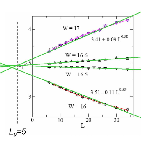
Figure 1: 3D data for $z_{1}=2L/\xi_{1D}$ [4] and their fitting by dependence $C(L+L_{0})$.

Our paper [1] contains the detailed predictions of the self-consistent theory of localization for the quantities which are immediately measured in numerical experiments; it allows to make a comparison on the level of the raw data, avoiding the ambiguous treatment procedure. Such approach is motivated by the different status of numerical results. The raw data are obtained independently by different groups and there is a certain consensus in this respect; it is not reasonable to question these data. However, it is possible to doubt numerical algorithms themselves, which are not based on a firm theoretical ground. Such approach is in the own interests of numerical researches since their present-day results contradict both experiment and the general theoretical principles. Self-consistent theory by Vollhardt and W${\rm{\ddot{o}}}$lfle allows to justify (for the first time) one of the popular variants of finite-size scaling based on consideration of auxiliary quasi-1D systems [2, 3] with a finite transverse size $L$. This theory predicts also the essential scaling corrections, so the scaling parameter has a behavior $C(L+L_{0})$ with $L_{0}>0$ in the vicinity of transition, which can be practically interpreted as $CL^{1/\nu}$ with $\nu>1$. Consideration of existing numerical data shows that there are no serious contradictions of the self-consistent theory with the raw numerical data.

Of course, it does not prove a validity of the self-consistent theory: deviations can be small but significant, and a serious analysis is necessary. The analysis of this kind is expected from the specialists in numerical research, such as P. Markos. In fact, in the comment [4] he makes no efforts to follow our suggestions but restricts himself by the ”standard scaling formulas”. First of all, there are no ”standard scaling formulas”, since corrections to scaling certainly exist and no reliable procedure to deal with them is available. Further, the conventional scaling is certainly invalid for dimensions $d>4$: it is a theorem [1]. Finally, we did not deny in [1] the possibility to fit the data by a simple power law dependence but stressed ambiguity of such procedure. From this point of view, FIGS. 2–5 in [4] have no relation to the criticism of the paper [1].

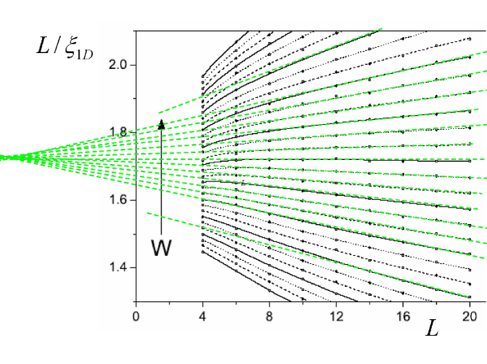
Figure 2: The same, as in Fig. 1, with smaller $L$ and higher accuracy (from the paper by Kramer et al [5]). For small deviations from the critical point the data are fitted well by dependence $C(L+L_{0})$. When deviations become large, dependencies acquire essential curvature, while effective $L_{0}$ changes significantly. Compare with Fig. 1.

3D system. In this case, P. Markos provides not a very essential progress: he extends his results till $L=34$, while data up to $L=50$ were discussed in [1]. Our interpretation of 3D data is presented in Fig. 1. The following points should be noted:

(a) The most interesting question is: does $L_{0}$ reveal an essential drift when the range of $L$ is extended? If we try to retain the estimate $L_{0}=5$ obtained in [1] for $L\leq 24$, then the data for $W=16.5$ and $16.6$ are fitted well with such restriction.

(b) The data for $W=16$ and $W=17$ show certain deviations from the linear behavior but they are not very impressive, since the scattering of points is rather large.

(c) In fact, the data for $W=16$ and $W=17$ contain the effect of the $W$ nonlinearity. If we suggest $\nu=1$, then $\xi\approx 30$ for $|W-W_{c}|=0.5$ and nonlinear effects are essential for $L\sim 30$. Fig. 1 confirms this conclusion, since the data for $W=16$ and $W=17$ are not symmetric relative to the curve $W=16.5$.  Deviations from the linear behavior are on the same level as violation of symmetry. It looks rather probable that for the more narrow interval (like $W=16.25\div 16.75$) fitting by the linear dependence will be satisfactory.  This argumentation is supported by other numerical data (Fig. 2).

Figure 3: 5D data for $z_{1}=2L/\xi_{1D}$ extracted from FIGS. 4, 5 in [4] (points) and their comparison with the scaling relation (2) (solid lines).

P. Markos has an illusion that the more complicated procedure allows to obtain the higher accuracy. In particular, in treatment of the $W$ dependence he relies on the quadratic expansion in $W-W_{c}$. In fact, one cannot exclude possibility that the coefficient of the quadratic term is small and the higher order corrections are essential. If different nonlinear functions are allowed, the uncertainty will be the same as for a simple linear fit in the more narrow interval. In the latter case, it is impossible to obtain a nonlinear behavior for the derivative $s(L)=\left[z_{1}(L)\right]^{\prime}_{\tau}$ from the apparently linear dependencies $z_{1}(L)$ (Fig. 2). With nonlinear treatment, P. Markos was able to do it (see FIG. 3 in [4]).

Comparison in FIG. 3 of [4] is not honest, since the dashed line does not correspond to predictions of [1]. The predicted dependence is $C(L+L_{0})$ and not $CL$, so the straight line with the unit slope is irrelevant. In fact, our concept works excellently in the range $L\leq 20$ (Fig. 2), where P. Markos shows disastrous deviations.

5D model. In this section we read:

”Our data in FIG.  4 do not indicate any discontinuity in the $L$ dependence. Contrary, $z_{1}$ is smooth analytical function of both parameters, $W$ and $L$.”

We do not predict any discontinuity, it is a fantasy by P. Markos. It is clear from Eq.45 in [1]

$$\tau\Lambda^{d-2}=\frac{1}{L^{d-2}}\,\frac{1}{2mL}-cm^{2}\Lambda^{d-4}$$

that $mL\equiv z_{1}$ is a regular function of $L$ and $\tau=W-W_{c}$. A singularity is developed only in the thermodynamic limit $L\to\infty$, as in all scaling theories. Modifications suggested for $d>4$ correspond to the usual scaling constructions, but in other variables

$$y=\frac{\xi_{1D}}{L}\left(\frac{a}{L}\right)^{(d-4)/3}\,,\qquad x=\frac{\xi}{L}\left(\frac{a}{L}\right)^{(d-4)/3}\,.$$

The scaling relation is found in the analytical form

$$\pm\frac{1}{x^{2}}=y-\frac{1}{y^{2}}\,,$$

where the proper scales for $\xi_{1D}$ and $\xi$ are chosen. Fig. 3 shows the quantity $z_{1}L^{1/3}\equiv 1/y$ as a function of $L$. Its dependence on $1/x\sim L^{4/3}$ has the same form but the logarithmic scale should be changed by the factor $4/3$. The solid lines correspond to the scaling relation (2). According to Fig. 3, the critical point is $W_{c}=53$ and not 57.5.

Conclusion. In this section, the author provides the additional argumentation:

”We also note that the same value of the critical exponent was obtained from numerical analysis of other physical quantities: mean conductance, conductance distribution, inverse participation ratio…”

In fact, two variants of scaling, (a) quasi-1D systems, and (b) level statistics, were discussed in [1]. The third variant, (c) mean conductance, is discussed in the recent paper [6]. The rest two variants, (d) conductance distribution [7], and (e) inverse participation ratio [8], are illustrated in Figs. 4 and 5. One can see, that our conception is supported by high-precision data with $L\leq 20$ and by moderate-precision data with $L\leq 50$.

Figure 4: Data for the conductance distribution [7] and their fitting by dependence $C(L+L_{0})$. The scaling parameter is the 0.17 percentile of distribution.

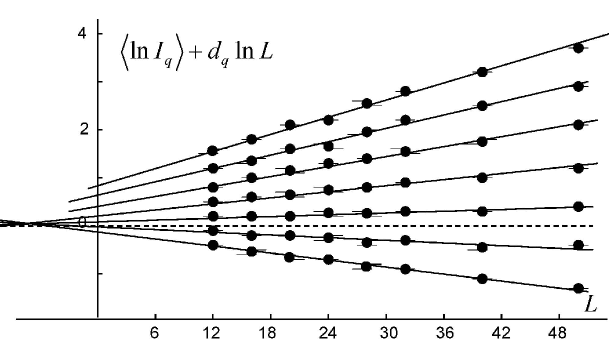
Figure 5: Data for the inverse participation ratio $I_{q}$ with $q=5$ extracted from Fig.2 in [8] and their fitting by dependence $C(L+L_{0})$. The essential change of $L_{0}$ is visible for large deviations from the critical point. The contribution $-d_{q}\ln L$ ($d_{q}$ is a fractal dimension) corresponds to the critical point.

The final arguments are also not serious:

”This value of the critical exponent was recently verified experimentally ^[11] and calculated analytically ^[12]”

The papers ^[11] deal with a quasiperiodic kicked rotor, whose equivalence with the 3D Anderson model is only a hypothesis essentially based on the questinable numerical data.  The real experiments on disordered systems [10, 11, 12] support the results of the self-consistent theory.

The ”analytical” result ^[12] violates the Wegner scaling relation $s=\nu(d-2)$, which is admitted by all serious theoreticians. Its violation means incorrectness of the one-parameter scaling hypothesis [13], which is a basis for practically all numerical studies.

In conclusion, P. Markos does not see the central idea of the paper [1] and continue to use the sophisticated treatment procedure instead of direct comparison on the level of raw data. If the latter is made, all existing numerical data look perfectly compatible with predictions of the self-consistent theory of localization.

References

- [1] I. M. Suslov, J. Exp. Theor. Phys. 114, 107 (2012) [Zh. Eksp. Teor. Fiz. 141, 122 (2012)]; arXiv: 1104.0432.
- [2] J. L. Pichard, G. Sarma, J. Phys. C: Solid State Phys. 14, L127 (1981); 14, L617 (1981).
- [3] A. MacKinnon, B. Kramer, Phys. Rev. Lett. 47, 1546 (1981); Z. Phys. 53, 1 (1983).
- [4] P. Markos, arXiv: 1205.0689.
- [5] B. Kramer, A. MacKinnon, K. Slevin, T. Ohtsuki, arXiv: 1004.0285
- [6] I. M. Suslov, arXiv: 1204.5169.
- [7] K. Slevin, P. Markos, T. Ohtsuki, Phys. Rev. b 67, 155106 (2003).
- [8] J. Brndiar, P. Markos, cond-mat/0606056.
- [9] I. M. Suslov, Zh. Eksp. Teor. Fiz. 83, 1079 (1982); 84, 1792 (1983) [Sov. Phys. JETP 56, 612 (1982); 57, 1044 (1983)].
- [10] D. Belitz, T. R. Kirkpatrick, Rev. Mod. Phys., 66, 261 (1994).
- [11] N. G. Zhdanova, M. S. Kagan, E. G. Landsberg, JETP 90, 662 (2000).
- [12] S. Waffenschmidt, C. Pfleiderer, H. V. Loehneysen, Phys. Rev. Lett. 83, 3005 (1999).
- [13] E. Abrahams, P. W. Anderson, D. C. Licciardello, and T. V. Ramakrishman, Phys. Rev. Lett. 42, 673 (1979).
- [14]