Majorana state on the surface of a disordered 3D topological insulator

Abstract

We study low-lying electron levels in an “antidot” capturing a coreless vortex on the surface of a three-dimensional topological insulator in the presence of disorder. The surface is covered with a superconductor film with a hole of size $R$ larger than coherence length, which induces superconductivity via proximity effect. Spectrum of electron states inside the hole is sensitive to disorder, however, topological properties of the system give rise to a robust Majorana bound state at zero energy. We calculate the subgap density of states with both energy and spatial resolution using the supersymmetric sigma model method. Tunneling into the hole region is sensitive to the Majorana level and exhibits resonant Andreev reflection at zero energy.

Topological insulators and superconductors are very peculiar materials with a gap in the bulk electron spectrum and a low-lying branch of subgap excitations on their surface (see reviewQiZhang for a review). This surface metallic state appears due to topological reasons and is robust with respect to any (sufficiently small) perturbations. In particular, topological properties prevent these surface states from Anderson localization. One common example of a topological insulator is a two-dimensional system in the integer quantum Hall effect regime. The bulk of such a system has a spectral gap between successive Landau levels and is hence an insulator. At the same time quantized Hall conductance appears due to a fixed integer number of chiral propagating edge modes on the background of the bulk gap. This type of materials are referred to as $\mathbb{Z}$ topological insulators.

Another type of topological insulator is realized in three-dimensional (3D) semiconductor crystals with sufficiently strong spin-orbit interaction (BiSb, BiTe, BiSe, strained HgTe etc). The spin-orbit interaction leads to inversion of the spectral gap. As a result subgap surface excitations appear with a dispersion of the massless Dirac type. The topological invariant in these materials has a $\mathbb{Z}_{2}$ nature. When the number of surface states is odd, one of them always remains gapless due to topological protection.

A general classification of topological insulators was developed in Refs. Kitaev ; Schnyder based on the symmetry of the underlying Hamiltonian. The quantum Hall effect is an example of a topologically nontrivial state of the unitary symmetry (class A of the Altland-Zirnbauer classification AltlandZirnbauer ) in 2D. Strong spin-orbit interaction leads to a topological state in the symplectic class (AII) in 3D. Another important example is the 1D topological superconductor of the class BD symmetry (superconductor with both time-reversal and spin rotation symmetries broken). The topologically protected mode in this case is zero-dimensional and is known as the Majorana bound state (MBS). It appears, in particular, in the core of an Abrikosov vortex in the spinless $p$-wave superconductor Ivanov00 . A similar MBS appears FuKane2008 in a vortex in an ordinary $s$-wave superconductor brought in contact with the surface of a 3D $\mathbb{Z}_{2}$ topological insulator, which corresponds to the symmetry class AII. The MBS appears as a descendant of the topologically protected massless Dirac state on the free surface of the topological insulator.

There are two general methods to observe the Majorana level. One of them relates to the anomalous Josephson effect kane4pi ; IoselFeig2011 . Another, and a more direct, way involves tunneling into the region where the MBS is supposed to be localized kouwenhoven . The differential conductance in such a tunneling experiment yields the local density of states with spatial and energy resolution. The Majorana state in the vortex core manifests itself by resonant Andreev reflection at zero energy LeeNg .

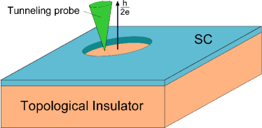
Figure 1: (Color online) A sketch of the considered setup. Three-dimensional topological insulator is covered by a superconducting film with a hole of radius $R$. The gap in the density of states is induced on the covered surface forming an antidot and confining surface excitations inside the hole. External magnetic field induces an Abrikosov vortex inside the hole. The spectrum of energy eigenstates inside the hole acquires a Majorana zero level which can be accessed in the tunneling measurement.

In this Letter we study local tunneling conductance for a setup depicted in Fig. 1. A superconducting (with a spectral gap $\Delta$) film with a circular hole of the radius $R$ is deposited on the surface of a 3D topological insulator, e.g., Bi₂Te₃ crystal. Perpendicular magnetic field applied to the system produces a vortex pinned to the hole. The radius $R$ is supposed to be relatively large, $R\geq(l,\xi_{0})$, where $l$ is the mean free path for topological insulator surface states and $\xi_{0}$ is the superconducting coherence length of the film. The condition $R\geq\xi_{0}$ allows one to avoid Melnikov the abundance of low-lying Caroli-de Gennes-Matricon states whose presence in the core of the Abrikosov vortex complicates observation of the $E=0$ Majorana state. Under these conditions disorder is relevant for the states localized in the hole region. Although the Majorana state is protected against disorder, i.e. its energy stays exactly zero, the spatial distribution of its wavefunction $\psi_{0}(\mathbf{r})$, and thus the local tunneling conductance are sensitive to disorder. The aim of this Letter is to calculate the tunneling conductance in the “dirty-limit” with spatial and energy resolution, and to identify the effects of the Majorana zero-energy state in the presence of strong disorder.

The problem is described by the following Bogolyubov-de Gennes (BdG) Hamiltonian in polar coordinates $r$, $\varphi$:

$$H=\begin{pmatrix}H_{0}&\Delta(r)e^{i\varphi}\\ \Delta(r)e^{-i\varphi}&-H_{0}\end{pmatrix},\quad H_{0}=v_{0}\,\mathbf{s}\cdot\mathbf{p}+V(\mathbf{r})-\mu.$$ (1)

Here the Hamiltonian $H_{0}$ describes the dynamics of surface excitations in a topological insulator without a superconducting layer. The Fermi velocity of surface electrons is denoted by $v_{0}$, $\mathbf{s}$ is the spin operator, and $V(\mathbf{r})$ is the random disorder potential. The Fermi level is shifted from the Dirac point by $\mu$. The vector potential term in $H_{0}$ is neglected due to smallness of magnetic field. We assume the dirty limit with a disorder induced mean free path $l\ll\xi=\sqrt{\hbar D/\Delta}$ and a relatively large hole with $R\gg\xi$; here $D=v_{0}^{2}\tau/2$. These conditions allow us to use a step-like radial dependence of the order parameter:

$$\Delta(r)=\begin{cases}0,&r<R,\\ \Delta,&r>R.\end{cases}$$ (2)

Inside the hole, the order parameter is zero and electron dynamics is governed by $H_{0}$. This Hamiltonian possesses time-reversal symmetry of the symplectic type, $H_{0}=s_{y}H_{0}^{*}s_{y}$, and hence belongs to the symplectic symmetry class AII. Proximity to the superconductor induces a gap in the electronic spectrum outside the hole. This gap effectively confines the low-lying excitations and imposes boundary conditions for the Hamiltonian $H_{0}$ at $r=R$. These boundary conditions break time-reversal symmetry due to the spatially rotating phase of the order parameter. At the same time the total BdG Hamiltonian $H$ acquires a specific particle-hole symmetry:

$$H=-s_{y}\tau_{y}H^{*}s_{y}\tau_{y}.$$ (3)

Here $\tau_{y}$ is the Pauli matrix acting in Nambu-Gor’kov (NG) space. Identity (3) implies a symmetry of the electron spectrum. For each eigenstate $\psi$ with energy $E$ there is a conjugate eigenstate $s_{y}\tau_{y}\psi^{*}$ with energy $-E$.

The particle-hole symmetry (3) defines the class BD. On the level of random matrices there are two distinct versions of this class with even and odd number of eigenstates referred to as D and B class, respectively. In class B, one unpaired eigenstate has exactly zero energy and is self-conjugate: $\psi=s_{y}\tau_{y}\psi^{*}$. The BdG Hamiltonian counts every physical excitation twice due to the doubling in NG space. An unpaired level is thus “half” of a true excitation — a Majorana state.

We will calculate the density of states inside the hole with the help of the supersymmetric non-linear sigma model. Two-dimensional Dirac fermions with potential disorder are described by a very peculiar model of the class AII with $\mathbb{Z}_{2}$ topological term Ostrovsky . This topological term appears as a consequence of the chiral anomaly of Dirac fermions. We will consider the minimal model operating with the $8\times 8$ supermatrix $Q$. Apart from Fermi-Bose superspace, this matrix operates in the space of retarded-advanced (RA) fields and in a specific time-reversal (TR) space introduced to take into account Cooperons and diffusons on equal footing. RA space is completely analogous to the NG space (see below); we denote Pauli matrices in this space by $\tau$. Notation $\sigma$ is used for Pauli matrices in TR space. A detailed derivation of the sigma model can be found in supplement .

In class AII, the matrix $Q$ obeys the non-linear constraint $Q^{2}=1$ and the linear constraint

$$Q=\bar{Q}\equiv CQ^{T}C^{T},\qquad C=\tau_{x}\begin{pmatrix}\sigma_{x}&0\\ 0&i\sigma_{y}\end{pmatrix}_{\text{FB}}.$$ (4)

As a result, $Q$ contains $8$ commuting and $8$ anticommuting (Grassmann) variables in total. Commuting degrees of freedom parameterize diagonal fermion-fermion (F) and boson-boson (B) blocks of $Q$. The general $Q$-matrix can be decomposed as

$$Q=U^{-1}\begin{pmatrix}Q_{\text{F}}&0\\ 0&Q_{\text{B}}\end{pmatrix}U,$$ (5)

where the central part contains only commuting variables while Grassmann parameters define the unitary supermatrix $U$. We will use the following explicit form of the central part of $Q$ in terms of eight angle parameters:

$$Q_{\text{F}} =[\tau_{z}\cos\theta_{f}+\sigma_{z}\sin\theta_{f}(\tau_{x}\cos\phi_{f}+\tau_{y}\sin\phi_{f})]$$

$$\;\;\,\times[\sigma_{z}\cos k_{f}+\tau_{z}\sin k_{f}(\sigma_{x}\cos\chi_{f}+\sigma_{y}\sin\chi_{f})],$$ (6)

$$Q_{\text{B}} =\tau_{z}\cos\theta_{b}[\sigma_{z}\cos k_{b}+\sin k_{b}(\sigma_{x}\cos\chi_{b}+\sigma_{y}\sin\chi_{b})]$$

$$\;\;\,+\sin\theta_{b}(\tau_{x}\cos\phi_{b}+\tau_{y}\sin\phi_{b}).$$ (7)

This representation fulfills all the constraints imposed by the symmetry class AII of the Hamiltonian $H_{0}$. The F and B sectors of the sigma model are compact and non-compact, respectively. This is achieved by demanding that the angles $\theta_{b}$, $k_{b}$ are imaginary while all other angles in Eqs. (6), (7) are real. Below we will find that the saddle point describing the density of states in the hole occurs with real $\theta_{b}$. This implies a proper shift of the integration contour for this angle.

The sigma model of class AII is designed to study transport properties of a disordered system. This implies that the $Q$ matrix operates, in particular, in the RA space allowing for averaging the product of retarded and advanced Green functions. We are interested in the density of states and hence it suffices to average just the single retarded function. At the same time, superconducting boundary conditions implemented in the BdG Hamiltonian (1) require to introduce an additional doubling of fields in the Nambu-Gor’kov space. This can be achieved within the standard AII class sigma model with the $8\times 8$ supermatrix $Q$ while the role of NG space is taken over by the RA structure of $Q$ (for detailed discussion of the transformation from RA to NG representation see supplement ; KoziiSkvor ).

Thus we can incorporate the superconducting order parameter directly into the action of the sigma model,

$$S[Q]=\frac{\pi\nu}{8}\!\int\!d^{2}r\mathop{\mathrm{Str}}\left[D(\nabla Q)^{2}+4(i\epsilon\Lambda-\hat{\Delta})Q\right]+S_{\theta}[Q],$$

$$\Lambda=\tau_{z}\sigma_{z},\qquad\hat{\Delta}=\Delta(r)(\tau_{x}\cos\varphi-\tau_{y}\sin\varphi).$$ (8)

Here $\epsilon=E+iG_{t}\delta(\mathbf{r}-\mathbf{r}_{0})/4\pi\nu$ is the sum of the energy $E$ and the local dwell term describing the coupling to a tunnel tip with dimensionless conductance $G_{t}\ll 1$ supplement .

The action (8) involves the $\mathbb{Z}_{2}$ topological term $S_{\theta}[Q]$ which appears due to massless Dirac nature of underlying electrons as was discussed above. The topological term involves only the compact part of the sigma-model manifold, i.e., its F sector $\mathcal{M}_{\text{F}}$. In the general version of the sigma model, that is capable of averaging several retarded and advanced Green functions, the homotopy group is $\pi_{2}(\mathcal{M}_{\text{F}})=\mathbb{Z}_{2}$. However, in the minimal model we are considering, $\mathcal{M}_{\text{F}}$ has the structure of the product of two spheres $S^{2}\times S^{2}$ as seen from Eq. (6). In this case the homotopy group is richer, $\mathbb{Z}\times\mathbb{Z}$. Two integer topological invariants can be introduced counting the degree of covering of the two spheres by the mapping $Q$ from real space to $\mathcal{M}_{\text{F}}$. This allows us to write the topological term explicitly although in a non-invariant form. With the parameterization (6), it reads (cf. Ref. Ostrovsky ):

$$S_{\theta}[Q]=\frac{i}{4}\int d^{2}r\Big{[}\sin\theta_{f}\big{(}\nabla\theta_{f}\times\nabla\phi_{f}\big{)}\\ +\sin k_{f}\big{(}\nabla k_{f}\times\nabla\chi_{f}\big{)}\Big{]}.$$ (9)

Let us now analyze the minima of the action (8) for the setup Fig. 1. Circular symmetry of the problem fixes the phase equal to the polar angle, $\phi_{f,b}=\varphi$. The other parameters depend only on the radial coordinate $r$. Both angles $\theta$ in F and B sectors obey the Usadel equation

$$D\left[\frac{\partial^{2}\theta}{\partial r^{2}}+\frac{1}{r}\,\frac{\partial\theta}{\partial r}-\frac{\sin 2\theta}{2r^{2}}\right]\\ +2iE\sin\theta\cos k+2\Delta(r)\cos\theta=0.$$ (10)

Inside the hole $\Delta=0$. At low energies we can also neglect the $E$ term and the equation becomes independent of $k$. The step-like dependence of the order parameter, Eq. (2), imposes the boundary condition $\theta(R)=\pi/2$. There are two possible solutions to the Usadel equation with this boundary condition:

$$\theta_{1} =2\arctan(r/R),$$ (11)

$$\theta_{2} =\pi-2\arctan(r/R).$$ (12)

Saddle point equations also require $k_{f}=0$ and hence the angle $\chi_{f}$ drops from the matrix $Q$ and from the action. The two remaining angles $k_{b}$ and $\chi_{b}$ are free and can take any constant values.

The spatial profile of $Q$ is thus fixed by the Usadel equation. The solutions $\theta_{1,2}$ represent two disconnected saddle points in the F sector while in the B sector only the saddle point $\theta_{b}=\theta_{1}$ is reachable. If the integration contour for $\theta_{b}$, which runs along the imaginary axis, is shifted to the point $\theta_{2}$ a divergence occurs in the $k_{b}$ integral. Thus the B sector is reduced to a hyperboloid parameterized by $ik_{b}>0$ and $0<\chi_{b}<2\pi$, see Ref. supplement . This is exactly the structure of the sigma model of class BD as we anticipated from symmetry analysis. The distinction between even (D) and odd (B) versions of this class is related to the disjoint character of the manifold due to the discrete degree of freedom in the F sector. Namely, in class D (B) the two parts of the manifold contribute to the partition function with the same (opposite) sign. In our problem the odd symmetry class B occurs. To demonstrate it, we compare the value of the action (8) at the two minima in the F sector. These two solutions indeed contribute with the opposite sign since the corresponding values of the topological term (9) differ by exactly $i\pi$.

The density of states is given by the integral

$$\rho(E,r)=\frac{\nu}{8}\mathop{\mathrm{Re}}\int DQ\mathop{\mathrm{Str}}[k\Lambda Q(r)]\;e^{-S[Q]}.$$ (13)

At low energies, this integral is to be calculated over the saddle manifold. Apart from the two variables $k_{b}$ and $\chi_{b}$ and two disconnected points in the F sector this manifold involves two Grassmann variables in the matrix $U$, Eq. (5). In order not to spoil the saddle point, these variables must be constant in space and fulfill the condition $[U,\hat{\Delta}]=0$. We introduce them according to

$$U=\exp\left[\frac{1}{2}\begin{pmatrix}0&\eta\sigma_{x}+\zeta\sigma_{y}\\ i\zeta\sigma_{x}-i\eta\sigma_{y}&0\end{pmatrix}_{\text{FB}}\right].$$ (14)

Within this parameterization, we can rewrite the integral (13) in terms of $k_{b}$, $\chi_{b}$, $\eta$, $\zeta$. Thus the problem is reduced to the 0D sigma model of class B (the two disjoint points in the F sector contribute with opposite signs). Explicit calculation of the integral IvanovSUSY ; supplement yields the local DOS in the factorized form

$$\rho(r,E)=\nu\,n(r)f(E/\omega_{0}),$$ (15)

$$n(r)=\cos\theta_{1}(r)=\frac{R^{2}-r^{2}}{R^{2}+r^{2}},$$ (16)

$$f(x)=\frac{\gamma}{\pi(x^{2}+\gamma^{2})}+1-\frac{\sin(2\pi x)}{2\pi x}.$$ (17)

Here $\gamma=G_{t}n(r_{0})/2\pi\ll 1$ and the low-energy level spacing is given by

$$\omega_{0}^{-1}=2\nu\int d^{2}r\,\cos\theta_{1}(r)=2\pi(\log 4-1)\nu R^{2}.$$ (18)

The spatial profile of DOS, $n(r)$, is fixed by the solution of the Usadel equation, while the energy dependence is characteristic for the B class and contains a narrow lorentzian peak at zero energy. This peak is the zero-energy MBS broadened due to the finite tunneling time. Note that the width $\gamma$ is position-dependent.

Integrating $\rho(r,E)$ over space yields the global DoS

$$N(E)=\frac{f(E/\omega_{0})}{2\omega_{0}}.$$ (19)

In the extreme tunneling limit $\gamma\to 0$, this function acquires the contribution $\delta(E)/2$ and coincides with the result IvanovSUSY up to a factor $2$ due to BdG double counting. The Majorana state appears as a half of a fermionic level.

Spatial and energy dependence of $\rho(r,E)$ factorize at energies much less than the Thouless energy $E_{\text{Th}}=D/R^{2}$. At higher energies fluctuations of $Q$ are not important and DOS is given just by a single saddle point. Approximate solution of the Usadel equation (10) in the limit $E\gg E_{\text{Th}}$ yields supplement

$$N(E\gg E_{\text{Th}})=\pi\nu R^{2}\left[1-\big{(}2-\sqrt{2}\big{)}\sqrt{E_{\text{Th}}/E}\right].$$ (20)

Local DOS is close to the normal value $\nu$ everywhere except for a narrow vicinity of the hole boundary.

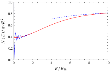
Figure 2: (Color online) Global density of states as a function of energy $E$. The solid blue oscillating curve represents the low-energy result (19), the dashed curve shows the high-energy asymptotics (20), and the red curve presents numerical solution interpolating between the two limits.

The local density is measured in the tunneling experiment. The tunneling current is determined by

$$I=\frac{eG_{t}}{2\pi\hbar\nu}\int\rho(E,r_{0})\big{[}f(E-eV)-f(E)\big{]}dE$$ (21)

with $f(E)$ being the equilibrium Fermi distribution function. At low temperatures and voltages, $(T,eV)\ll\omega_{0}$, we keep only the first lorentzian term in the energy dependence of the local DOS (17). The differential conductance exhibits a peak

$$\frac{dI}{dV}=\begin{cases}\dfrac{e^{2}\gamma^{2}}{\pi\hbar\big{[}\gamma^{2}+(eV/\omega_{0})^{2}\big{]}},&T\ll\gamma\omega_{0},\\ \dfrac{e^{2}\gamma\omega_{0}}{4\hbar T\cosh^{2}(eV/2T)},&\gamma\omega_{0}\ll T\ll\omega_{0}.\end{cases}$$ (22)

At very low temperatures the height of this peak is universal and equals $e^{2}/\pi\hbar$. This signifies resonant Andreev reflection at the Majorana state. This effect in the absence of disorder was studied in Ref. LeeNg . At larger (and more realistic) temperatures, $\gamma\omega_{0}\ll T\leq\omega_{0}$, the height of the peak is parametrically small, $dI/dV\sim\gamma\omega_{0}/T$.

Noise power of the tunneling current in the same regime $(T,eV)\ll\omega_{0}$ is supplement

$$S(V,T,r_{0})=\frac{e^{2}\gamma\omega_{0}}{2\hbar},\qquad\gamma\omega_{0}\ll T\ll\omega_{0}.$$ (23)

The noise produced by the Majorana level is $T$- and $V$-independent as long as $\gamma\omega_{0}\ll T$.

The results (22) and (23) apply at low temperature and voltage. When temperature and/or voltage are higher than the level spacing $\omega_{0}$, non-zero-energy states also contribute to the tunneling current. Positions and widths of these states depend on the realization of disorder. For low temperature but high voltage, $T<\omega_{0}<eV$, narrow resonances similar to Eq. (22) will occur due to non-zero levels Paper2 . Positions of these resonances strongly depend on disorder realization; their heights are smaller but close to $e^{2}/\pi\hbar$ and widths are of order $\gamma\omega_{0}$. When temperature exceeds $\omega_{0}$, all the resonances get smeared and the normal average DOS $\nu$ is recovered.

To conclude, we have studied the local density of states in the superconducting vortex on the surface of a topological insulator in the superconducting antidot setup depicted in Fig. 1. The spatial and energy dependence of the density of states factorize at low energies and the latter is given by the 0D sigma model of symmetry class B. We have identified the zero-energy Majorana state occurring due to the topological properties of the system. This Majorana state exhibits itself via the resonant Andreev reflection at zero energy yielding the peak in differential conductance with the universal amplitude $e^{2}/\pi\hbar$ and width proportional to the normal conductance $G_{t}$.

We are grateful to B. Sacepe for stimulating discussions. This work was supported by the RFBR grant 10-02-00554-a and by the German Ministry of Education and Research (BMBF).

Supplementary Information

.1 Derivation of the sigma-model

.1.1 Sigma model for hybrid structure

In this section we derive the sigma model describing the dynamics of the topological insulator surface excitations in the presence of a random potential. We assume the hole geometry depicted in Fig. 1 of the main text. The derivation starts with the microscopic Bogolyubov – de Gennes Hamiltonian (1). The sigma model is aimed at averaging the single retarded Green function determining the density of states. We will also demonstrate the equivalence of this sigma model to the model of the symplectic symmetry class AII describing the transport properties of massless Dirac fermions. The latter model is based on the normal, rather than superconducting, Hamiltonian and is capable of calculating averaged products of retarded and advanced Green functions. It is known that the sigma model for Dirac fermions possesses the specific $\mathbb{Z}_{2}$ topological term. The equivalence of the two models will prove the appearance of the topological term in the superconducting case considered in the present paper.

Let us start with the retarded Green function in the system governed by the Hamiltonian (1). We will use the supersymmetric integral representation

$$G^{R}_{E}(\mathbf{r},\mathbf{r}^{\prime})=-i\int D\Phi^{*}\,D\Phi\,\mathop{\mathrm{str}}\left[k\Phi(\mathbf{r})\Phi^{\dagger}(\mathbf{r}^{\prime})\right]e^{-S},\qquad\qquad S=-i\int d^{2}r\,\Phi^{\dagger}\big{(}E+i0-H\big{)}\Phi.$$ (24)

Here the vector fields $\Phi$ and $\Phi^{\dagger}$ contain $4$ commuting and $4$ Grassmann parameters each. Apart from the spin and Bogolyubov – de Gennes structure of the Hamiltonian, we also introduce the superstructure in order to get rid of the normalizing denominator and facilitate further disorder averaging. The pre-exponential factor contains the supermatrix $k=\{1,-1\}_{\text{FB}}$ and supertrace is defined as in Ref. Efetov : $\mathop{\mathrm{str}}A=A_{\text{FF}}-A_{\text{BB}}$.

The superconducting symmetry of the Hamiltonian $H$, Eq. (3), gives rise to specific soft modes – Cooperons – of the type $\langle G^{R}_{E}G^{R}_{-E}\rangle$. These modes are relevant for the average density of states since they are built out of retarded functions only. In order to include them into our effective theory, we transform the action by writing half of it in the form (24) and another half in the time-reversed (transposed) form:

$$S=-\frac{i}{2}\int d^{2}r\Big{[}\Phi^{\dagger}\big{(}E+i0-H\big{)}\Phi-\Phi^{T}k\big{(}E+i0+s_{y}\tau_{y}Hs_{y}\tau_{y}\big{)}\Phi^{*}\Big{]}\\ =-\frac{i}{2}\int d^{2}r\begin{pmatrix}\Phi^{+}\tau_{z},&i\Phi^{T}ks_{y}\tau_{x}\end{pmatrix}\left[(E+i0)\sigma_{z}\tau_{z}-H_{0}-\tau_{z}\hat{\Delta}\right]\begin{pmatrix}\Phi\\ s_{y}\tau_{y}\Phi^{*}\end{pmatrix}.$$ (25)

Here we have introduced the matrix $\sigma_{z}$ operating in the space of time-reversed blocks – TR space. The matrix $k$ appeared due to anticommutation of Grassmann variables. We will denote the doubled vectors as

$$\Psi=\frac{1}{\sqrt{2}}\begin{pmatrix}\Phi\\ s_{y}\tau_{y}\Phi^{*}\end{pmatrix},\qquad\qquad\bar{\Psi}=\frac{1}{\sqrt{2}}\begin{pmatrix}\Phi^{+}\tau_{z},&i\Phi^{T}ks_{y}\tau_{x}\end{pmatrix}.$$ (26)

They are no longer independent, as $\Phi$ and $\Phi^{*}$ were, but rather obey the linear constraint

$$\bar{\Psi}=(C\Psi)^{T},\qquad\qquad C=-is_{y}\tau_{x}\begin{pmatrix}\sigma_{x}&0\\ 0&i\sigma_{y}\end{pmatrix}_{\text{FB}}.$$ (27)

At this stage, we are ready to perform the disorder averaging. We adopt the standard Gaussian white noise disorder model characterized by the correlator

$$\langle V(\mathbf{r})V(\mathbf{r}^{\prime})\rangle=\frac{\delta(\mathbf{r}-\mathbf{r}^{\prime})}{\pi\nu\tau}.$$ (28)

The single-particle density of states is defined as $\nu=|\mu|/2\pi v_{0}^{2}$. Note that the right-hand side is twice bigger compared to the standard definition applied to normal metals. The reason for this extra factor $2$ is the Dirac nature of electron spectrum and hence doubling of the phase space due to the two types of excitations (electrons and holes).

Disorder averaging produces the quartic term in the action,

$$S=\int d^{2}r\left\{\frac{(\bar{\Psi}\Psi)^{2}}{2\pi\nu\tau}-i\bar{\Psi}\left[(E+i0)\Lambda+\mu-v_{0}\,\mathbf{s}\cdot\mathbf{p}-\tau_{z}\hat{\Delta}\right]\Psi\right\}.$$ (29)

Here we use the notation $\Lambda=\sigma_{z}\tau_{z}$. The interaction term is further decoupled with the help of the Hubbard-Stratonovich transformation by introducing an auxiliary matrix field $Q$. The construction of the nonlinear sigma model implies that the field $Q$ contains all relevant slow modes of the disordered system – diffusons and Cooperons. There are in total three ways to decouple the four-fermion interaction Efetov . One of them involves a scalar field $\sim\langle\bar{\Psi}\Psi\rangle$ analogous to the random potential $V$. This leads only to an irrelevant renormalization of the chemical potential. Two other decoupling schemes introduce a matrix field with the structure $\langle\Psi\bar{\Psi}\rangle$ and $\langle\Psi\Psi^{T}\rangle$ corresponding to diffusons and Cooperons, respectively. In order to include all relevant slow modes in the theory, we have to perform decoupling in both ways, which can be achieved with a single matrix $Q$. Details of this calculation can be found in Ref. Efetov . The resulting action has the form:

$$S=\frac{\pi\nu}{16\tau}\mathop{\mathrm{str}}Q^{2}-i\int d^{2}r\,\bar{\Psi}\left[E\Lambda+\mu-v_{0}\,\mathbf{s}\cdot\mathbf{p}-\tau_{z}\hat{\Delta}+\frac{iQ}{2\tau}\right]\Psi.$$ (30)

The vectors $\Psi$ and $\bar{\Psi}$ are related by Eq. (27). This allows us to limit the matrix $Q$ by the linear constraint $Q=\bar{Q}\equiv CQ^{T}C^{T}$. This relation keeps only those parameters in $Q$ that couple to the product $\Psi\bar{\Psi}$. Integrating out the field $\Psi$ yields the action for the matrix $Q$:

$$S=\frac{\pi\nu}{16\tau}\mathop{\mathrm{str}}Q^{2}-\frac{1}{2}\mathop{\mathrm{str}}\ln\left[E\Lambda+\mu-v_{0}\,\mathbf{s}\cdot\mathbf{p}-\tau_{z}\hat{\Delta}+\frac{iQ}{2\tau}\right].$$ (31)

Derivation of the sigma model proceeds with the saddle-point analysis of the above action. In the dirty limit, the energy and $\hat{\Delta}$ terms in the argument of the logarithm are relatively small compared to $Q/\tau$. With these small terms neglected, the action possesses the uniform saddle point $Q=\Lambda$. This saddle point corresponds to the self energy of the average electron Green function in the self-consistent Born approximation. Other saddle points can be achieved by rotations $Q=T^{-1}\Lambda T$, if the matrix $T$ commutes with the spin operator $\mathbf{s}$ ($E$ and $\Delta$ terms are still neglected). Rotations $T$ define the target manifold of the non-linear sigma model. The effective action of the sigma model within this manifold is derived with the help of the gradient expansion of Eq. (31) allowing for slow spatial variation of $Q$ and perturbative expansion to the linear order in $E$ and $\hat{\Delta}$. Since the $Q$ matrix is trivial in the spin space, we can safely reduce its size to $8\times 8$ keeping only Nambu, TR, and FB structure. Then the self-conjugacy relation acquires the form of Eq. (4).

The gradient expansion of Eq. (31) is a highly nontrivial procedure in view of the chiral anomaly of the Dirac fermions. The momentum integrals arising after the expansion of the logarithm are divergent in the ultraviolet limit and require a proper regularization. The result of the expansion is independent of a particular regularization scheme provided the gauge invariance is preserved. The anomaly affects only the imaginary part of the action and leads to the appearance of the topological term Ostrovsky . At the same time, the real part can be obtained in a straightforward way since all the arising momentum integrals are convergent. The result reads

$$\mathop{\mathrm{Re}}S=\frac{\pi\nu}{8}\int d^{2}r\mathop{\mathrm{str}}\left[D(\nabla Q)^{2}+4i(E\Lambda-\tau_{z}\hat{\Delta})Q\right].$$ (32)

Here the diffusion coefficient is $D=v_{0}^{2}\tau/2$ and the matrix $Q$ is reduced to the $8\times 8$ size. The action (8), used in the main text, differs from Eq. (32) only by a $\pi/2$ rotation of the superconducting phase and by an imaginary contribution to the energy term. The latter corresponds to a finite dwell time of the electron due to the coupling to the tunneling microscope tip as we elaborate below.

In order to explain the emergence of the topological term in the imaginary part of the action, we will prove the equivalence of the sigma model, derived here for the hybrid structure of Fig. 1, to the symplectic sigma model for Dirac fermions derived in Ref. Ostrovsky .

.1.2 Sigma model for Dirac fermions

The sigma model obtained by the gradient expansion of Eq. (31) belongs to the symplectic symmetry class AII. This is quite natural since the Hamiltonian possesses only time-reversal symmetry in the absence of the $\hat{\Delta}$ term. Let us demonstrate the equivalence between our sigma model (8) describing the density of states for the Hamiltonian $H$, Eq. (1), and the standard symplectic class sigma model describing transport via the surface states of the topological insulator with Hamiltonian $H_{0}$. In the latter case, the sigma model yields averaged products of retarded and advanced Green functions with the energy difference $\omega$. This requires introducing retarded-advanced (RA) structure of the action,

$$S_{0}=-i\int d^{2}r\,\Phi^{\dagger}\tau_{z}\big{[}(\omega/2+i0)\tau_{z}-H_{0}\big{]}\Phi.$$ (33)

Here the matrix $\tau_{z}$ operates in the RA space. Subscript $0$ is used to distinguish this model from the sigma model derived in the previous section and used in the main text.

The time-reversal symmetry $H_{0}=s_{y}H_{0}^{T}s_{y}$ is taken into account by further doubling of variables in the TR space,

$$S_{0}=-\frac{i}{2}\int d^{2}r\Big{[}\Phi^{\dagger}\big{(}\omega/2+i0-\tau_{z}H_{0}\big{)}\Phi-\Phi^{T}k\big{(}\omega/2+i0-\tau_{z}s_{y}H_{0}s_{y}\big{)}\Phi^{*}\Big{]}\\ =-\frac{i}{2}\int d^{2}r\begin{pmatrix}\Phi^{\dagger}\tau_{z},&i\Phi^{T}ks_{y}\tau_{z}\end{pmatrix}\big{[}(\omega/2+i0)\Lambda_{0}-H_{0}\big{]}\begin{pmatrix}\Phi\\ is_{y}\Phi^{*}\end{pmatrix}.$$ (34)

Note that the matrix $\Lambda_{0}=\tau_{z}$ multiplying the frequency term is different from its counterpart $\Lambda$ from the previous section. The vectors $\Psi$ and $\bar{\Psi}$ as well as the charge conjugation matrix $C_{0}$ are also defined differently,

$$\Psi=\frac{1}{\sqrt{2}}\begin{pmatrix}\Phi\\ is_{y}\Phi^{*}\end{pmatrix},\qquad\qquad\bar{\Psi}=(C_{0}\Psi)^{T}=\frac{1}{\sqrt{2}}\begin{pmatrix}\Phi^{+}\tau_{z},&i\Phi^{T}ks_{y}\tau_{z}\end{pmatrix},\qquad\qquad C_{0}=-is_{y}\tau_{z}\begin{pmatrix}\sigma_{x}&0\\ 0&i\sigma_{y}\end{pmatrix}_{\text{FB}}.$$ (35)

Already at this stage we can prove the equivalence of the two models by selecting a proper unitary rotation of the field vector $\Psi$. This unitary rotation should obey the following properties:

$$U^{T}C_{0}U=C,\qquad\qquad U^{-1}\Lambda_{0}U=\Lambda.$$ (36)

These relations bring the charge conjugation matrix $C_{0}$ and the matrix $\Lambda_{0}$ to the representation used in the previous section for the sigma model of the hybrid system. There are many matrices $U$ that fulfill identities (36). One possible choice is

$$U=\begin{pmatrix}1&0\\ 0&i\tau_{y}\end{pmatrix}_{\text{TR}}.$$ (37)

In the case of usual rather than Dirac fermions, an analogous equivalence between the sigma model for the density of states in a superconducting hybrid structure and the orthogonal class sigma model is discussed in Ref. KoziiSkvor .

.1.3 Topological term

So far we have discussed the derivation of the real part of the sigma-model action (8) and also proved the equivalence of this model to the symplectic class sigma model for Dirac fermions (up to the boundary conditions involving the term $\hat{\Delta}$). The latter model is known to possess the $\mathbb{Z}_{2}$ topological term as an imaginary part of its action, see Ref. Ostrovsky . This allows us to include the topological term in the action (8) and thus complete its derivation.

The explicit form of the topological term is written in the main text, Eq. (9), in a noninvariant form, using the parameterization (5) – (7). In this section we will discuss an indirect but explicitly invariant representation of this topological term.

The target manifold of the symplectic class sigma model is fixed by the representation $Q=T^{-1}\Lambda T$ with the constraint $Q=\bar{Q}$. If we neglect the Grassmann parameters and consider the central part of $Q$, see Eq. (5), these conditions yield $Q_{\text{F}}\in O(4)/O(2)\times O(2)$ and $Q_{\text{B}}\in Sp(2,2)/Sp(2)\times Sp(2)$. The topological term arises in the compact F sector of the model. An explicit expression for the topological term can be written within a construction similar to the Wess-Zumino-Witten term, cf. Ref. Konig .

We first extend the target manifold by relaxing the condition $Q^{2}=1$. Let us introduce the matrix $\mathcal{Q}=\bar{T}\Lambda T$. The only restriction on this matrix is $\mathcal{Q}=\bar{\mathcal{Q}}$. The F sector of the extended manifold is $\mathcal{Q}_{\text{F}}\in O(4)$. It has trivial second homotopy group, $\pi_{2}[O(4)]=0$. This allows us to introduce the third, auxiliary, coordinate $0\leq t\leq 1$, such that the real 2D space corresponds to $t=1$, and continuously extend the matrix field according to

$$\mathcal{Q}(\mathbf{r},t)=\begin{cases}Q(\mathbf{r}),&t=1,\\ \Lambda,&t=0.\end{cases}$$ (38)

Such an extension assumes that the physical space has no boundary and can be viewed as a surface of a 3D ball with $t$ being the radial coordinate. With this definition of $\mathcal{Q}$, the Wess-Zumino-Witten term has the form

$$S_{\theta}[Q]=\frac{i\epsilon_{abc}}{24\pi}\int_{0}^{1}dt\int d^{2}r\mathop{\mathrm{str}}\Big{[}\mathcal{Q}^{-1}(\nabla_{a}\mathcal{Q})\mathcal{Q}^{-1}(\nabla_{b}\mathcal{Q})\mathcal{Q}^{-1}(\nabla_{c}\mathcal{Q})\Big{]}.$$ (39)

Here the indices $a$, $b$, and $c$ take three values corresponding to the three coordinates $t$, $x$, and $y$, and $\epsilon_{abc}$ is the unit antisymmetric tensor.

The integrand in this expression (39) is a total derivative therefore the result of the integration depends only on the value of $\mathcal{Q}$ at the boundary of integration domain, i.e., on the physical field $Q=\mathcal{Q}|_{t=1}$. This can be checked by an explicit calculation of the variation of $S_{\theta}$:

$$\delta S_{\theta}[Q]=\frac{i\epsilon_{abc}}{8\pi}\int_{0}^{1}dt\int d^{2}r\nabla_{a}\mathop{\mathrm{str}}\Big{[}\mathcal{Q}^{-1}\delta\mathcal{Q}\mathcal{Q}^{-1}(\nabla_{b}\mathcal{Q})\mathcal{Q}^{-1}(\nabla_{c}\mathcal{Q})\Big{]}=\frac{i}{8\pi}\int d^{2}r\mathop{\mathrm{str}}\Big{\{}Q^{-1}\delta Q\big{[}Q^{-1}(\nabla_{x}Q),Q^{-1}(\nabla_{y}Q)\big{]}\Big{\}}.$$ (40)

A topological term does not change under continuous variations of the field $Q$ but takes different values in different (disconnected) topological sectors of the model. The general Wess-Zumino-Witten term has a nonzero variation and hence does not obey this property. However, the term (39) is constrained by $Q^{2}=1$. Under this condition, the variation (40) is identically zero. Hence the Wess-Zumino-Witten term (39) indeed plays the role of a topological term.

The value of the topological term is quantized, yielding the topological charge of the field configuration, only in a system without boundary. This is not the case for the geometry considered in the paper. The matrix $Q$ is defined in the finite region inside the hole (see Fig. 1 of the main text) with the boundary conditions fixed by the $\hat{\Delta}$ term in the Hamiltonian (1). The value of the topological term is not completely fixed in this case. In particular, the expression (39) depends not only on physical values of $Q$ but also on the way it is extended in the third dimension, Eq. (38). However, this uncertainty leads only to an uncontrolled imaginary constant in the action. This constant is the same in both topological sectors of the model and hence does not alter any observable quantities.

An alternative derivation of the sigma-model action, including the topological term in the form Eq. (39) is possible within the non-abelian bosonization formalism. Let us for a moment assume, that the Hamiltonian has an extra chiral symmetry, $H=-s_{z}Hs_{z}$. This situation corresponds to the symmetry class DIII and can be realized, e.g., at the Dirac point in the presence of a random velocity disorder. The sigma model of the class DIII has an extended target space, corresponding to the manifold of $\mathcal{Q}$ introduced above. This sigma model possesses the Wess-Zumino-Witten term (39), see Ref. Witten , and is the result of the non-abelian bosonization of the initial fermionic problem. Non-zero chemical potential drives the system away from the Dirac point and breaks the chiral symmetry. This reduces the model to the symplectic symmetry class and restricts the field by the condition $Q^{2}=1$. The resulting action has the topological term in the form of the restricted Wess-Zumino-Witten term (39) as discussed above.

.1.4 Tunneling coupling term

In this section we discuss the appearance of the imaginary contribution to the energy due to the presence of the tunneling tip. In order to include the coupling to an external metallic probe, we extend the Hamiltonian as

$$\mathcal{H}=\begin{pmatrix}H&t\\ t^{\dagger}&H_{M}\end{pmatrix}.$$ (41)

Diagonal blocks of this matrix are the Hamiltonian $H$ of the topological insulator surface (1) and the Hamiltonian $H_{M}$ describing electron states in the metallic tip. Off-diagonal elements $t$ and $t^{\dagger}$ are tunneling amplitudes between the two subsystems. We assume these tunneling amplitudes are local in space and couple the states at point $r_{0}$ on the sample surface to the states at the tip of the metallic probe.

Deriving the sigma model as described in previous sections we arrive at the expression similar to Eq. (31) but with an extended matrix structure:

$$S=\frac{\pi\nu}{16\tau}\mathop{\mathrm{str}}Q^{2}+\frac{\pi\nu_{M}}{16\tau_{M}}\mathop{\mathrm{str}}Q_{M}^{2}-\frac{1}{2}\mathop{\mathrm{str}}\ln\left[E\Lambda-\tau_{z}\mathcal{H}+\begin{pmatrix}iQ/2\tau&0\\ 0&iQ_{M}/2\tau_{M}\end{pmatrix}\right].$$ (42)

The quantities $\nu_{M}$, $\tau_{M}$, and $Q_{M}$ refer to the metallic tip. In the absence of tunneling, $t=0$, the two subsystems decouple and we obtain independent sigma models describing topological insulator and the tip. We will assume the density of states $\nu_{M}$ to be large, that will fix $Q_{M}=\Lambda$. Tunneling coupling is assumed to be weak. This allows us to expand the logarithm in powers of $t$ and $t^{\dagger}$. The lowest non-vanishing contribution appears in the second order of the perturbation theory and yields the tunneling term in the sigma model,

$$S_{t}=\frac{1}{2}\mathop{\mathrm{str}}\Big{[}(E\Lambda-\tau_{z}H+iQ/2\tau)^{-1}\tau_{z}t(E\Lambda-\tau_{z}H_{M}+iQ_{M}/2\tau_{M})^{-1}\tau_{z}t^{\dagger}\Big{]}=-\frac{\pi^{2}}{8}\,\nu\nu_{M}\mathop{\mathrm{str}}\big{(}Q\tau_{z}tQ_{M}\tau_{z}t^{\dagger}\big{)}.$$ (43)

In the last expression we have used the saddle-point relation between $Q$ and the Green function $(E\Lambda-\tau_{z}H+iQ/2\tau)^{-1}$ in coincident points. We introduce normal dimensionless (in units $e^{2}/h$) tunnel conductance of the junction $G_{t}=\pi^{2}\nu\nu_{M}\mathop{\mathrm{tr}}(tt^{\dagger})$ (note that $\nu$ and $\nu_{M}$ are total rather than spinless densities of states at the Fermi energy). Assuming $Q_{M}=\Lambda$, we rewrite the action as

$$S_{t}=-\frac{G_{t}}{8}\mathop{\mathrm{str}}\Lambda Q.$$ (44)

Thus the tunneling term has the same structure as the energy term and produces an imaginary contribution to $E$, see Eq. (8) of the main text.

.2 Calculation of the density of states

.2.1 Low energies $E\ll E_{\text{Th}}$

The local density of states on the surface of the topological insulator is given by Eq. (13) of the main text. The integral over matrix $Q$ is to be calculated over the saddle manifold fixed by the solution of the Usadel equation (10). There are two distinct solutions $\theta_{1,2}$, [see Eqs. (11), (12) of the main text] for the angle $\theta_{\text{F}}$. In the F sector of the model, all other parameters are fixed and thus $\theta_{1,2}$ represent two disjoint parts of the integration manifold. At the same time, only the solution $\theta_{b}=\theta_{1}$ is allowed in the B sector, and two other angles, $k_{\text{B}}$ and $\chi_{\text{B}}$, are free forming a hyperboloid (the parameter $k_{\text{B}}$ must be imaginary in order to ensure convergence of the integral).

To calculate the density of states from Eq. (13), we have to express $\mathop{\mathrm{Str}}(k\Lambda Q(r))$, $S[Q]$ and $DQ$ in terms of $k_{b}$, $\chi_{b}$, $\eta$, and $\zeta$ for the two disjoint parts of the manifold. However, a direct use of our parameterization leads to an uncertainty in the integral over the part corresponding to $\theta_{f}=\theta_{2}$. The integral over $d\eta\,d\zeta$ is zero, while the integral over $k_{b}$ diverges. We resolve this uncertainty by a trick proposed in Ref. IvanovSUSY . The two disjoint parts of the integration manifold can be mapped onto each other by the similarity transformation

$$Q\mapsto T^{-1}QT,\qquad\qquad T=\begin{pmatrix}\sigma_{x}&0\\ 0&1\end{pmatrix}_{\text{FB}}.$$ (45)

We use the parametrization (6), (7) in the domain with $\theta_{f}=\theta_{1}$ and then apply the transformation (45) to cover the second topological sector with $\theta_{f}=\theta_{2}$. Owing to the relation (45), integration measure is the same in both sectors. It is given by the superdeterminant of the metric tensor in the space of $Q$ matrices, see Ref. Efetov . The integration measure reads

$$DQ=\frac{1}{2\pi}\,\tanh\frac{\kappa}{2}\,d\kappa\,d\chi_{b}\,d\eta\,d\zeta,$$ (46)

with $\kappa=ik_{b}$ ($k_{b}$ is imaginary to ensure the convergence of the integral). The integration runs over the hyperboloid $\kappa>0$, $0<\chi_{b}<2\pi$.

The action in the two topological sectors $\theta_{f}=\theta_{1,2}$ has the form

$$S_{1} =-4i\pi\nu\int d^{2}r\,\epsilon\cos\theta_{1}\left(\sinh^{2}\frac{\kappa}{2}-i\eta\zeta\cosh^{2}\frac{\kappa}{2}\right)-\frac{i\pi}{2}=-2i\pi\tilde{x}\left(\sinh^{2}\frac{\kappa}{2}-i\eta\zeta\cosh^{2}\frac{\kappa}{2}\right)-\frac{i\pi}{2},$$ (47)

$$S_{2} =-4i\pi\nu\int d^{2}r\,\epsilon\cos\theta_{1}\,\cosh^{2}\frac{\kappa}{2}-\frac{i\pi}{2}=-2i\pi\tilde{x}\cosh^{2}\frac{\kappa}{2}+\frac{i\pi}{2}.$$ (48)

Here we have introduced the complex dimensionless energy parameter $\tilde{x}=\int d^{2}r\,\epsilon\cos\theta_{1}=x+i\gamma$, with the real part $x=E/\omega_{0}$ [see Eq. (18) in the main text] and the imaginary part $\gamma=G_{t}n(r_{0})/2\pi$. The latter appears due to the coupling to the tunneling tip. The terms $\pm i\pi/2$ in Eqs. (47), (48) appear due to the topological term $S_{\theta}[Q]$, see Eq. (9). With the above expressions for $DQ$ and the action we can calculate the total partition function of the theory,

$$\int DQ\,e^{-S[Q]}=\int_{0}^{\infty}\tanh\frac{\kappa}{2}\,d\kappa\,d\eta\,d\zeta\exp\left[2i\pi\tilde{x}\left(\sinh^{2}\frac{\kappa}{2}-i\eta\zeta\cosh^{2}\frac{\kappa}{2}\right)+\frac{i\pi}{2}\right]=1.$$ (49)

This is exactly what one expects for the partition function of a supersymmetric theory. Note that the topologically nontrivial sector does not contribute to this result since the action $S_{2}$ contains no Grassmann variables.

In order to calculate the density of states, we need the pre-exponential factor from Eq. (13). In our parameterization, it has the following form in the two sectors:

$$\frac{\nu}{8}\mathop{\mathrm{Str}}(k\Lambda Q)=\nu\cos\theta_{1}\times\begin{cases}\cosh^{2}\dfrac{\kappa}{2},&\theta_{f}=\theta_{1},\\[8.0pt] \sinh^{2}\dfrac{\kappa}{2}-i\eta\zeta cosh^{2}\dfrac{\kappa}{2},&\theta_{f}=\theta_{2}.\end{cases}$$ (50)

$$\rho=\nu\cos\theta_{1}\mathop{\mathrm{Re}}\int_{0}^{\infty}\tanh\frac{\kappa}{2}\,d\kappa\,d\eta\,d\zeta\Bigg{\{}\cosh^{2}\frac{\kappa}{2}\exp\left[2i\pi\tilde{x}\left(\sinh^{2}\frac{\kappa}{2}-i\eta\zeta\cosh^{2}\frac{\kappa}{2}\right)+\frac{i\pi}{2}\right]\\ +\left(\sinh^{2}\frac{\kappa}{2}-i\eta\zeta\cosh^{2}\frac{\kappa}{2}\right)\exp\left[2i\pi\tilde{x}\cosh^{2}\frac{\kappa}{2}-\frac{i\pi}{2}\right]\Bigg{\}}\\ =\nu\cos\theta_{1}\mathop{\mathrm{Re}}\int_{0}^{\infty}d\kappa\,\cosh\frac{\kappa}{2}\sinh\frac{\kappa}{2}\Bigg{[}-2i\pi\tilde{x}\cosh^{2}\frac{\kappa}{2}\exp\left(2i\pi\tilde{x}\sinh^{2}\frac{\kappa}{2}\right)+\exp\left(2i\pi\tilde{x}\cosh^{2}\frac{\kappa}{2}\right)\Bigg{]}\\ =\nu\cos\theta_{1}\left(1-\mathop{\mathrm{Re}}\frac{1+e^{2i\pi\tilde{x}}}{2i\pi\tilde{x}}\right)=\nu\cos\theta_{1}\left[1+\frac{\gamma}{\pi(x^{2}+\gamma^{2})}-\frac{\sin(2\pi x)}{2\pi x}\right].$$ (51)

In the last expression we have used the condition $\gamma\ll 1$. The result (51) coincides with Eqs. (15) – (17) of the main text. In the tunneling limit $\gamma\to 0$ the lorentzian term yields a delta function. This implies that the Majorana state is robust in a closed system and disorder does not smear it.

Note, that for an alternative model of the symmetry class D, when the topological term is absent, the density of states does not contain the Majorana delta-peak. Two topological sectors contribute with the same sign yielding IvanovSUSY

$$\rho_{D}=\nu\cos\theta_{1}\left[1+\frac{\sin(2\pi x)}{2\pi x}\right].$$ (52)

.2.2 High energies $E_{\text{Th}}\ll E\ll\Delta$

In the previous section, we have calculated the density of states at low energies. The result (51) exhibits a delta-peak at zero energy and oscillations which decay at the characteristic energy scale $\omega_{0}$. These oscillations appear due to repulsion between low-lying levels with energies $E$ and $-E$. The scale $\omega_{0}$ is the global mean level spacing inside the hole. At higher energies $E\gg\omega_{0}$, the effect of level repulsion can be neglected and the density of states is given by the mean-field expression

$$\rho(r,E)=\nu\mathop{\mathrm{Re}}\cos\theta(r,E),$$ (53)

where $\theta$ is a solution of the Usadel equation (10) with $k=0$. The result (53) can be obtained from the sigma model identity (13) by integrating over $Q$ around the unique global minimum of the action given by the Usadel equation. Supersymmetry ensures that the integration with respect to small fluctuations around the minimum yields unity and hence Eq. (53) follows.

The Usadel equation is a complicated non-linear equation that cannot be solved analytically for arbitrary $E$. At relatively low energies $\omega_{0}\ll E\ll E_{\text{Th}}$, the solution can be found perturbatively in $E$. While linear correction in $E$ to $\theta$ is purely imaginary and does not change the density of states, the second order calculation up to terms $\sim E^{2}$ is necessary to obtain the observable result. The spatial profile of this small energy correction does not factorize as in the main term, see Eq. (15) in the main text. Second order perturbation theory amounts to solving linear differential equations, obtained by linearizing Eq. (10), and leads to very complicated functions. We will not discuss any further details of this approach here.

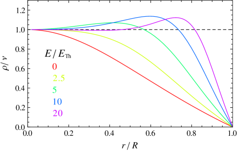
Figure 3: Spatial dependence of the density of states for different values of $E$. At lowest energies, the result (16) of the main text is reproduced, while at energies well above $E_{\text{Th}}$ the density of states is depleted only close to the hole edge within the strip $\sim R\sqrt{E_{Th}/E}$ in agreement with Eq. (55). Remarkably, the density of states is first increased above its normal value before dropping to zero at $r=R$.

As the energy is increased further and exceeds the Thouless energy, $E_{\text{Th}}\ll E\ll\Delta$, the Usadel equation admits another approximate solution. The angle $\theta$ is small everywhere except a narrow vicinity of the hole boundary. In this vicinity we can neglect the curvature of the superconductor edge and write an approximate one-dimensional Usadel equation

$$D\,\frac{\partial^{2}\theta}{\partial r^{2}}+2iE\sin\theta=0.$$ (54)

With the boundary conditions $\theta(R)=\pi/2$ and $\theta(r\ll R)\to 0$, solution to this equation reads

$$\theta=4\arctan\left[(\sqrt{2}-1)\exp\left[\sqrt{-2i\frac{E}{E_{\text{Th}}}}\left(\frac{r}{R}-1\right)\right]\right].$$ (55)

The density of states is given by Eq. (53) with the above result for $\theta$. We see that $\theta$ decreases from $\pi/2$ down to exponentially small values in a narrow strip of the width $\sim R\sqrt{E_{\text{Th}}/E}$ near the hole boundary. The density of states takes its normal value $\nu$ everywhere inside the hole except for this narrow strip where it is depleted down to zero. Spatial integration yields global density of states

$$N(E\gg E_{\text{Th}})=\pi\nu R^{2}\left[1-(2-\sqrt{2})\sqrt{\frac{E_{\text{Th}}}{E}}\right].$$ (56)

This is the result (20) of the main text.

We have also solved the Usadel equation numerically for the whole range of energies below $\Delta$. The spatial profile of the density of states is shown in Fig. 3 and the energy dependence of global DOS is depicted in Fig. 2 in the main text. It perfectly matches both the low-energy limit (up to delta peak and oscillatory term) of Eq. (15) and high-energy asymptotics (56).

.3 Tunneling current and noise

Tunneling current and noise can be found using the Landauer formalism instead of the sigma model. Electrons incident from the metallic probe are either reflected normally or experience Andreev reflection. Amplitudes of these processes can be found from the microscopic Hamiltonian of the system and used to calculate the current and higher cumulants, such as noise. The current $I(V)$ found this way coincides with the result derived from the sigma model and presented in the main text, Eq. (21). The noise, Eq. (23), was found by means of the Landauer approach since the sigma-model consideration of this problem is rather cumbersome. A detailed derivation of the Landauer formalism for our problem and the calculation of current and noise will be presented elsewhere Paper2 .

References

- (1) X.-L. Qi, S.-C. Zhang, Rev. Mod. Phys. 83, 1057 (2011).
- (2) A. Kitaev, AIP Conf. Proc. 1134, 22 (2009).
- (3) A. P. Schnyder, et al., Phys. Rev. B 78, 195125 (2008).
- (4) A. Altland and M. Zirnbauer, Phys. Rev. B 55, 1142 (1997).
- (5) D. Ivanov, Phys. Rev. Lett. 86, 268 (2001).
- (6) L. Fu and C. L. Kane, Phys. Rev. Lett. 100, 096407 (2008).
- (7) L. Fu and C. L. Kane, Phys. Rev. B 79, 161408 (2009).
- (8) P. A. Ioselevich and M. V. Feigel’man, Phys. Rev. Lett. 106, 077003 (2011).
- (9) V. Mourik et al., Science 1222360 (2012).
- (10) K. T. Law, P. A. Lee, and T. K. Ng, Phys. Rev. Lett. 103, 237001 (2009).
- (11) A. S. Mel’nikov, A. V. Samokhvalov, M. N. Zubarev, Phys. Rev. B 79, 134529 (2009).
- (12) P. M. Ostrovsky, I. V. Gornyi, and A. D. Mirlin, Phys. Rev. Lett. 105, 036803 (2010).
- (13) For details of sigma model derivation and calculation of the density of states see supplementary material.
- (14) V. Koziy and M. A. Skvortsov, JETP Lett. 94, 222 (2011).
- (15) D. A. Ivanov, J. Math. Phys. 43, 126 (2002).
- (16) P. A. Ioselevich and M. V. Feigel’man, to be published.

References

- (1) K. B. Efetov, Supersymmetry in Disorder and Chaos (Cambridge University Press, New York, 1997).
- (2) E. J. König, P. M. Ostrovsky, I. V. Protopopov, A. D. Mirlin, arXiv:1201.6288.
- (3) E. Witten, Commun. Math. Phys. 92, 455 (1984).