On optimal direction gibbs sampling

J. Andrés Christen(a), Colin Fox(b),
Diego Andrés Pérez-Ruiz(a) and Mario Santana-Cibrian(a)
(a) Centro de Investigación en Matemáticas (CIMAT),
A.P. 402, Guanajuato, Gto. 36000, Mexico. jac@cimat.mx
(b) Colin Fox, Department of Physics, University of Otago,
New Zealand. fox@physics.otago.ac.nz
Corresponding author.
(May 2012)
Abstract

Generalized Gibbs kernels are those that may take any direction not necessarily bounded each axis along the parameters of the objective function. We study how to optimally choose such directions in a Directional, random scan, Gibbs sampler setting. The optimal direction is chosen by minimizing to the mutual information (Kullback-Leibler divergence) of two steps of the MCMC for a truncated Normal objective function. The result is generalized to be used when a Multivariate Normal (local) approximation is available for the objective function. Three Gibbs direction distributions are tested in highly skewed non-normal objective functions.

Keywords: MCMC; Bayesian inference; simulation.

1 Introduction

Let π(𝒙)𝜋𝒙\pi(\boldsymbol{x}) be the objective distribution of interest. Let 𝑿n𝑿superscript𝑛\boldsymbol{X}\in\mathbb{R}^{n} be a random variable with density π(𝒙)𝜋𝒙\pi(\boldsymbol{x}). The (univariate) Gibbs sampler is a MCMC sampling algorithm that simulates systematically or randomly from the conditional distributions

fXi|𝑿i(xi|𝒙i)π(𝒙),proportional-tosubscript𝑓conditionalsubscript𝑋𝑖subscript𝑿𝑖conditionalsubscript𝑥𝑖subscript𝒙𝑖𝜋𝒙f_{X_{i}|\boldsymbol{X}_{-i}}(x_{i}|\boldsymbol{x}_{-i})\propto\pi(\boldsymbol{x}), (1)

where the notation

𝒗i=(v1,,vi1,vi+1,,vn)subscript𝒗𝑖subscript𝑣1subscript𝑣𝑖1subscript𝑣𝑖1subscript𝑣𝑛\boldsymbol{v}_{-i}=(v_{1},\ldots,v_{i-1},v_{i+1},\ldots,v_{n})

represents the (n1)𝑛1(n-1)-dimension vector created by deleting the i𝑖i-th entry from the n𝑛n-dimension vector 𝒗𝒗\boldsymbol{v}. (1) above represent univariate distributions and are the conditional distributions alone the axis for the base chosen to represent 𝑿𝑿\boldsymbol{X}, the so called full conditional distributions.

Using (1) a Markov chain 𝑿(1),𝑿(2),superscript𝑿1superscript𝑿2\boldsymbol{X}^{(1)},\boldsymbol{X}^{(2)},\ldots is created considering the transition kernel

Ki(𝒙(t),𝒙(t+1))=fXi|𝑿i(xi(t+1)|𝒙i(t))1(𝒙i(t+1)=𝒙i(t)).subscript𝐾𝑖superscript𝒙𝑡superscript𝒙𝑡1subscript𝑓conditionalsubscript𝑋𝑖subscript𝑿𝑖conditionalsubscriptsuperscript𝑥𝑡1𝑖subscriptsuperscript𝒙𝑡𝑖1subscriptsuperscript𝒙𝑡1𝑖subscriptsuperscript𝒙𝑡𝑖K_{i}(\boldsymbol{x}^{(t)},\boldsymbol{x}^{(t+1)})=f_{X_{i}|\boldsymbol{X}_{-i}}(x^{(t+1)}_{i}|\boldsymbol{x}^{(t)}_{-i})1(\boldsymbol{x}^{(t+1)}_{-i}=\boldsymbol{x}^{(t)}_{-i}).

That is, the i𝑖i-th kernel changes only the i𝑖i-th coordinate by simulating from the full conditional distribution fXi|𝑿i(|𝒙i(t))f_{X_{i}|\boldsymbol{X}_{-i}}(\cdot|\boldsymbol{x}^{(t)}_{-i}). In random scan Gibbs, a complete transition kernel is defined as

K(𝒙,𝒚)=i=1nwiKi(𝒙,𝒚),𝐾𝒙𝒚superscriptsubscript𝑖1𝑛subscript𝑤𝑖subscript𝐾𝑖𝒙𝒚K(\boldsymbol{x},\boldsymbol{y})=\sum_{i=1}^{n}w_{i}K_{i}(\boldsymbol{x},\boldsymbol{y}),

for some weights i=1nwi=1superscriptsubscript𝑖1𝑛subscript𝑤𝑖1\sum_{i=1}^{n}w_{i}=1; wi0subscript𝑤𝑖0w_{i}\geq 0.

The direction Gibbs sampler generalizes this idea by choosing a direction 𝒆n𝒆superscript𝑛\boldsymbol{e}\in\mathbb{R}^{n}, 𝒆=1norm𝒆1||\boldsymbol{e}||=1, and sampling from the conditional distribution alone such direction. This can be written as

𝑿(t+1)=𝒙(t)+r𝒆,superscript𝑿𝑡1superscript𝒙𝑡𝑟𝒆\boldsymbol{X}^{(t+1)}=\boldsymbol{x}^{(t)}+r\boldsymbol{e},

where the length r𝑟r\in\mathbb{R} has distribution proportional to π(𝒙(t)+r𝒆)𝜋superscript𝒙𝑡𝑟𝒆\pi(\boldsymbol{x}^{(t)}+r\boldsymbol{e}). In any case, it can be seen that the transition kernel has detailed balance with respect to π𝜋\pi, and by assuring π𝜋\pi-irreducibility the Markov chain has π𝜋\pi as ergodic distribution.

The natural question to ask is how to choose 𝒆𝒆\boldsymbol{e} to optimize the convergence (mixing) of the Markov chain? Indeed, once irreducibility is assured, any chain will have the correct ergodic distribution (π𝜋\pi) but performance will depend on how dependent 𝑿(t+1)superscript𝑿𝑡1\boldsymbol{X}^{(t+1)} and 𝑿(t)superscript𝑿𝑡\boldsymbol{X}^{(t)} are. In this context a convenient, although less known, dependence measure to use is the mutual information I𝐼I between random variables X𝑋X and Y𝑌Y, which measures the Kullback-Leibler divergence between the joint model fX,Ysubscript𝑓𝑋𝑌f_{X,Y} and the independent alternative fXfYsubscript𝑓𝑋subscript𝑓𝑌f_{X}f_{Y}, that is,

I(𝒀,𝑿)=f𝒀,𝑿(𝒚,𝒙)logf𝒀,𝑿(𝒚,𝒙)f𝒀(𝒚)f𝑿(𝒙)d𝒙d𝒚.𝐼𝒀𝑿subscript𝑓𝒀𝑿𝒚𝒙subscript𝑓𝒀𝑿𝒚𝒙subscript𝑓𝒀𝒚subscript𝑓𝑿𝒙𝑑𝒙𝑑𝒚I(\boldsymbol{Y},\boldsymbol{X})=\int\int f_{\boldsymbol{Y},\boldsymbol{X}}(\boldsymbol{y},\boldsymbol{x})\log\frac{f_{\boldsymbol{Y},\boldsymbol{X}}(\boldsymbol{y},\boldsymbol{x})}{f_{\boldsymbol{Y}}(\boldsymbol{y})f_{\boldsymbol{X}}(\boldsymbol{x})}d\boldsymbol{x}d\boldsymbol{y}.

In our case, this translates to 𝑿=𝑿(t)𝑿superscript𝑿𝑡\boldsymbol{X}=\boldsymbol{X}^{(t)} and 𝒀=𝑿(t+1)𝒀superscript𝑿𝑡1\boldsymbol{Y}=\boldsymbol{X}^{(t+1)}. Assuming that 𝑿πsimilar-to𝑿𝜋\boldsymbol{X}\sim\pi, we see that f𝒀(𝒚)=π(𝒚)subscript𝑓𝒀𝒚𝜋𝒚f_{\boldsymbol{Y}}(\boldsymbol{y})=\pi(\boldsymbol{y}) and f𝒀,𝑿(𝒚,𝒙)=π(𝒙)K(𝒙,𝒚)subscript𝑓𝒀𝑿𝒚𝒙𝜋𝒙𝐾𝒙𝒚f_{\boldsymbol{Y},\boldsymbol{X}}(\boldsymbol{y},\boldsymbol{x})=\pi(\boldsymbol{x})K(\boldsymbol{x},\boldsymbol{y}). Therefore, the mutual information above can be calculated as

I(𝒀,𝑿)=π(𝒙)K(𝒙,𝒚)logK(𝒙,𝒚)π(𝒚)d𝒚d𝒙.𝐼𝒀𝑿𝜋𝒙𝐾𝒙𝒚𝐾𝒙𝒚𝜋𝒚𝑑𝒚𝑑𝒙I(\boldsymbol{Y},\boldsymbol{X})=\int\int\pi(\boldsymbol{x})K(\boldsymbol{x},\boldsymbol{y})\log\frac{K(\boldsymbol{x},\boldsymbol{y})}{\pi(\boldsymbol{y})}d\boldsymbol{y}d\boldsymbol{x}. (2)

The idea would be to choose directions for which I(𝑿(t+1),𝑿(t))𝐼superscript𝑿𝑡1superscript𝑿𝑡I(\boldsymbol{X}^{(t+1)},\boldsymbol{X}^{(t)}) is minimized. Since I𝐼I is a Kullback-Leibler divergence it is well defined, I0𝐼0I\geq 0 and I=0𝐼0I=0 if and only if 𝑿(t+1)superscript𝑿𝑡1\boldsymbol{X}^{(t+1)} and 𝑿(t)superscript𝑿𝑡\boldsymbol{X}^{(t)} are independent (fX,Y=fXfYsubscript𝑓𝑋𝑌subscript𝑓𝑋subscript𝑓𝑌f_{X,Y}=f_{X}f_{Y} a.s.). Finding directions 𝒆𝒆\boldsymbol{e} for which I𝐼I is minimum will provide our optimization criterion, to obtaining better suited direction Gibbs samplers.

2 The Normal case

In many applications, a Multivariate Normal approximation to the posterior is possible. We will try to use such Normal approximation to produce an improved Gibbs samplers. In this section we will assume π𝜋\pi to be Normal, a case that lends itself to calculate I(𝑿(t+1),𝑿(t))𝐼superscript𝑿𝑡1superscript𝑿𝑡I(\boldsymbol{X}^{(t+1)},\boldsymbol{X}^{(t)}). For the moment, we will consider that the dimension is sufficiently low so as to have the eigen decomposition of the precision matrix available.

We therefore assume that π𝜋\pi is a multi- variate Normal with precision (n×n𝑛𝑛n\times n) matrix 𝑨𝑨\boldsymbol{A} (the inverse of the variance-covariance matrix) and mean column vector 𝝁𝝁\boldsymbol{\mu}. As explained above, given a direction 𝒆n𝒆superscript𝑛\boldsymbol{e}\in\mathbb{R}^{n}, 𝒆=1norm𝒆1||\boldsymbol{e}||=1, the chain moves from 𝑿(t)=𝒙superscript𝑿𝑡𝒙\boldsymbol{X}^{(t)}=\boldsymbol{x} to

𝒀=𝑿(t+1)=𝒙+r𝒆,𝒀superscript𝑿𝑡1𝒙𝑟𝒆\boldsymbol{Y}=\boldsymbol{X}^{(t+1)}=\boldsymbol{x}+r\boldsymbol{e},

where the length r𝑟r\in\mathbb{R} has distribution g𝑔g proportional to π(𝒙+r𝒆)𝜋𝒙𝑟𝒆\pi(\boldsymbol{x}+r\boldsymbol{e}). That is

g(r)exp{12(𝒗+r𝒆)𝑨(𝒗+r𝒆)},proportional-to𝑔𝑟12superscript𝒗𝑟𝒆𝑨𝒗𝑟𝒆g(r)\propto\exp\left\{-\frac{1}{2}(\boldsymbol{v}+r\boldsymbol{e})^{\prime}\boldsymbol{A}(\boldsymbol{v}+r\boldsymbol{e})\right\},

where 𝒗=𝒙𝝁𝒗𝒙𝝁\boldsymbol{v}=\boldsymbol{x}-\boldsymbol{\mu}. After some algebra we see that rN(𝒆A𝒗𝒆A𝒆,𝒆A𝒆)similar-to𝑟𝑁superscript𝒆𝐴𝒗superscript𝒆𝐴𝒆superscript𝒆𝐴𝒆r\sim N\left(-\frac{\boldsymbol{e}^{\prime}A\boldsymbol{v}}{\boldsymbol{e}^{\prime}A\boldsymbol{e}},\boldsymbol{e}^{\prime}A\boldsymbol{e}\right), where 𝒆A𝒆superscript𝒆𝐴𝒆\boldsymbol{e}^{\prime}A\boldsymbol{e} is the precision (by setting 𝒆=𝒆i𝒆subscript𝒆𝑖\boldsymbol{e}=\boldsymbol{e}_{i}, the i𝑖i-th standard bases vector, one obtains

YiN(μiaii1(𝒗𝒗(xiμi)2),aii),similar-tosubscript𝑌𝑖𝑁subscript𝜇𝑖superscriptsubscript𝑎𝑖𝑖1superscript𝒗𝒗superscriptsubscript𝑥𝑖subscript𝜇𝑖2subscript𝑎𝑖𝑖Y_{i}\sim N\left(\mu_{i}-a_{ii}^{-1}(\boldsymbol{v}^{\prime}\boldsymbol{v}-(x_{i}-\mu_{i})^{2}),a_{ii}\right),

which is the full conditional distribution for a Multivariate Normal distribution for entry i𝑖i, thus returning to the usual Gibbs sampler). From this we see that the transition kernel corresponding to direction 𝒆𝒆\boldsymbol{e} is

K𝒆(𝒙,𝒚)=(𝒆𝑨𝒆2π)12exp{𝒆𝑨𝒆2(𝒆(𝒚𝒙)+𝒆𝑨𝒗𝒆𝑨𝒆)2}1(𝒚=𝒙+𝒆(𝒚𝒙)𝒆)subscript𝐾𝒆𝒙𝒚superscriptsuperscript𝒆𝑨𝒆2𝜋12superscript𝒆𝑨𝒆2superscriptsuperscript𝒆𝒚𝒙superscript𝒆𝑨𝒗superscript𝒆𝑨𝒆21𝒚𝒙superscript𝒆𝒚𝒙𝒆K_{\boldsymbol{e}}(\boldsymbol{x},\boldsymbol{y})=\left(\frac{\boldsymbol{e}^{\prime}\boldsymbol{A}\boldsymbol{e}}{2\pi}\right)^{1\over 2}\exp\left\{-\frac{\boldsymbol{e}^{\prime}\boldsymbol{A}\boldsymbol{e}}{2}\left(\boldsymbol{e}^{\prime}(\boldsymbol{y}-\boldsymbol{x})+\frac{\boldsymbol{e}^{\prime}\boldsymbol{A}\boldsymbol{v}}{\boldsymbol{e}^{\prime}\boldsymbol{A}\boldsymbol{e}}\right)^{2}\right\}1(\boldsymbol{y}=\boldsymbol{x}+\boldsymbol{e}^{\prime}(\boldsymbol{y}-\boldsymbol{x})\boldsymbol{e})

(note that 𝒚𝒙=r𝒆𝒚𝒙𝑟𝒆\boldsymbol{y}-\boldsymbol{x}=r\boldsymbol{e} and since 𝒆𝒆=1superscript𝒆𝒆1\boldsymbol{e}^{\prime}\boldsymbol{e}=1, r=𝒆(𝒚𝒙)𝑟superscript𝒆𝒚𝒙r=\boldsymbol{e}^{\prime}(\boldsymbol{y}-\boldsymbol{x}); therefore 𝒚𝒚\boldsymbol{y} is restricted to the line 𝒚=𝒙+𝒆(𝒚𝒙)𝒆𝒚𝒙superscript𝒆𝒚𝒙𝒆\boldsymbol{y}=\boldsymbol{x}+\boldsymbol{e}^{\prime}(\boldsymbol{y}-\boldsymbol{x})\boldsymbol{e}).

We calculate I𝒆(𝑿(t+1),𝑿(t))subscript𝐼𝒆superscript𝑿𝑡1superscript𝑿𝑡I_{\boldsymbol{e}}(\boldsymbol{X}^{(t+1)},\boldsymbol{X}^{(t)}), the mutual information of the Gibbs sampler given direction 𝒆𝒆\boldsymbol{e}, as in 2. Note that

logK𝒆(𝒙,𝒚)π(𝒚)=C+12log𝒆𝑨𝒆12(Q1(𝒆,𝒙,𝒚)Q2(𝒚)),subscript𝐾𝒆𝒙𝒚𝜋𝒚𝐶12superscript𝒆𝑨𝒆12subscript𝑄1𝒆𝒙𝒚subscript𝑄2𝒚\log\frac{K_{\boldsymbol{e}}(\boldsymbol{x},\boldsymbol{y})}{\pi(\boldsymbol{y})}=C+\frac{1}{2}\log\boldsymbol{e}^{\prime}\boldsymbol{A}\boldsymbol{e}-\frac{1}{2}\left(Q_{1}(\boldsymbol{e},\boldsymbol{x},\boldsymbol{y})-Q_{2}(\boldsymbol{y})\right),

where

C𝐶\displaystyle C =n12log2π12log|𝑨|,absent𝑛122𝜋12𝑨\displaystyle=\frac{n-1}{2}\log 2\pi-\frac{1}{2}\log\left|\boldsymbol{A}\right|,
Q1(𝒆,𝒙,𝒚)subscript𝑄1𝒆𝒙𝒚\displaystyle Q_{1}(\boldsymbol{e},\boldsymbol{x},\boldsymbol{y}) =𝒆𝑨𝒆(𝒆(𝒚𝒙)+𝒆𝑨𝒗𝒆𝑨𝒆)2,absentsuperscript𝒆𝑨𝒆superscriptsuperscript𝒆𝒚𝒙superscript𝒆𝑨𝒗superscript𝒆𝑨𝒆2\displaystyle=\boldsymbol{e}^{\prime}\boldsymbol{A}\boldsymbol{e}\left(\boldsymbol{e}^{\prime}(\boldsymbol{y}-\boldsymbol{x})+\frac{\boldsymbol{e}^{\prime}\boldsymbol{A}\boldsymbol{v}}{\boldsymbol{e}^{\prime}\boldsymbol{A}\boldsymbol{e}}\right)^{2},
Q2(𝒚)subscript𝑄2𝒚\displaystyle Q_{2}(\boldsymbol{y}) =(𝒚𝝁)𝑨(𝒚𝝁).absentsuperscript𝒚𝝁𝑨𝒚𝝁\displaystyle=(\boldsymbol{y}-\boldsymbol{\mu})^{\prime}\boldsymbol{A}(\boldsymbol{y}-\boldsymbol{\mu}).

From this we see that

logK𝒆(𝒙,𝒚)π(𝒚)K𝒆(𝒙,𝒚)𝑑𝒚=C12+12log𝒆𝑨𝒆+12Q2(𝒚)K𝒆(𝒙,𝒚)𝑑𝒚subscript𝐾𝒆𝒙𝒚𝜋𝒚subscript𝐾𝒆𝒙𝒚differential-d𝒚𝐶1212superscript𝒆𝑨𝒆12subscript𝑄2𝒚subscript𝐾𝒆𝒙𝒚differential-d𝒚\int\log\frac{K_{\boldsymbol{e}}(\boldsymbol{x},\boldsymbol{y})}{\pi(\boldsymbol{y})}K_{\boldsymbol{e}}(\boldsymbol{x},\boldsymbol{y})d\boldsymbol{y}=C-\frac{1}{2}+\frac{1}{2}\log\boldsymbol{e}^{\prime}\boldsymbol{A}\boldsymbol{e}+\frac{1}{2}\int Q_{2}(\boldsymbol{y})K_{\boldsymbol{e}}(\boldsymbol{x},\boldsymbol{y})d\boldsymbol{y}

since Q1(𝒆,𝒙,𝒚)K𝒆(𝒙,𝒚)𝑑𝒚=1subscript𝑄1𝒆𝒙𝒚subscript𝐾𝒆𝒙𝒚differential-d𝒚1\int Q_{1}(\boldsymbol{e},\boldsymbol{x},\boldsymbol{y})K_{\boldsymbol{e}}(\boldsymbol{x},\boldsymbol{y})d\boldsymbol{y}=1. The integral Q2(𝒚)K𝒆(𝒙,𝒚)𝑑𝒚subscript𝑄2𝒚subscript𝐾𝒆𝒙𝒚differential-d𝒚\int Q_{2}(\boldsymbol{y})K_{\boldsymbol{e}}(\boldsymbol{x},\boldsymbol{y})d\boldsymbol{y} may be calculated by transforming back to r𝑟r since

Q2(𝒚)K𝒆(𝒙,𝒚)𝑑𝒚=(r𝒆𝒗)𝑨(r𝒆𝒗)g𝒆(r)𝑑r.subscript𝑄2𝒚subscript𝐾𝒆𝒙𝒚differential-d𝒚superscript𝑟𝒆𝒗𝑨𝑟𝒆𝒗subscript𝑔𝒆𝑟differential-d𝑟\int Q_{2}(\boldsymbol{y})K_{\boldsymbol{e}}(\boldsymbol{x},\boldsymbol{y})d\boldsymbol{y}=\int(r\boldsymbol{e}-\boldsymbol{v})^{\prime}\boldsymbol{A}(r\boldsymbol{e}-\boldsymbol{v})g_{\boldsymbol{e}}(r)dr.

After some algebra one sees that

Q2(𝒚)K𝒆(𝒙,𝒚)𝑑𝒚=1𝒗𝑨𝒆𝒆𝑨𝒗𝒆𝑨𝒆+𝒗𝑨𝒗.subscript𝑄2𝒚subscript𝐾𝒆𝒙𝒚differential-d𝒚1superscript𝒗𝑨𝒆superscript𝒆𝑨𝒗superscript𝒆𝑨𝒆superscript𝒗𝑨𝒗\int Q_{2}(\boldsymbol{y})K_{\boldsymbol{e}}(\boldsymbol{x},\boldsymbol{y})d\boldsymbol{y}=1-\frac{\boldsymbol{v}^{\prime}\boldsymbol{A}\boldsymbol{e}\boldsymbol{e}^{\prime}\boldsymbol{A}\boldsymbol{v}}{\boldsymbol{e}^{\prime}\boldsymbol{A}\boldsymbol{e}}+\boldsymbol{v}^{\prime}\boldsymbol{A}\boldsymbol{v}.

Therefore

logK𝒆(𝒙,𝒚)π(𝒚)K𝒆(𝒙,𝒚)𝑑𝒚=C+12log𝒆𝑨𝒆12𝒗𝑨𝒆𝒆𝑨𝒗𝒆𝑨𝒆+𝒗𝑨𝒗.subscript𝐾𝒆𝒙𝒚𝜋𝒚subscript𝐾𝒆𝒙𝒚differential-d𝒚𝐶12superscript𝒆𝑨𝒆12superscript𝒗𝑨𝒆superscript𝒆𝑨𝒗superscript𝒆𝑨𝒆superscript𝒗𝑨𝒗\int\log\frac{K_{\boldsymbol{e}}(\boldsymbol{x},\boldsymbol{y})}{\pi(\boldsymbol{y})}K_{\boldsymbol{e}}(\boldsymbol{x},\boldsymbol{y})d\boldsymbol{y}=C+\frac{1}{2}\log\boldsymbol{e}^{\prime}\boldsymbol{A}\boldsymbol{e}-\frac{1}{2}\frac{\boldsymbol{v}^{\prime}\boldsymbol{A}\boldsymbol{e}\boldsymbol{e}^{\prime}\boldsymbol{A}\boldsymbol{v}}{\boldsymbol{e}^{\prime}\boldsymbol{A}\boldsymbol{e}}+\boldsymbol{v}^{\prime}\boldsymbol{A}\boldsymbol{v}.

We need now to integrate with respect to π(d𝒙)𝜋𝑑𝒙\pi(d\boldsymbol{x}). We note that 𝒗𝑨𝒗π(𝒙)𝑑𝒙=nsuperscript𝒗𝑨𝒗𝜋𝒙differential-d𝒙𝑛\int\boldsymbol{v}^{\prime}\boldsymbol{A}\boldsymbol{v}\pi(\boldsymbol{x})d\boldsymbol{x}=n. Moreover, the expected value of a quadratic form is

E(𝒛𝑹𝒛)=tr(𝑹𝚺)+𝝁𝑹𝝁,𝐸superscript𝒛𝑹𝒛𝑡𝑟𝑹𝚺superscript𝝁𝑹𝝁E(\boldsymbol{z}^{\prime}\boldsymbol{R}\boldsymbol{z})=tr(\boldsymbol{R}\boldsymbol{\Sigma})+\boldsymbol{\mu}^{\prime}\boldsymbol{R}\boldsymbol{\mu},

where 𝝁𝝁\boldsymbol{\mu} and 𝚺𝚺\boldsymbol{\Sigma} are the mean vector and the variance-covariance matrix of 𝒛𝒛\boldsymbol{z}. Letting 𝑹=𝑨𝒆𝒆𝑨𝒆𝑨𝒆𝑹𝑨𝒆superscript𝒆𝑨superscript𝒆𝑨𝒆\boldsymbol{R}=\frac{\boldsymbol{A}\boldsymbol{e}\boldsymbol{e}^{\prime}\boldsymbol{A}}{\boldsymbol{e}^{\prime}\boldsymbol{A}\boldsymbol{e}} and since E(𝒗)=𝟎𝐸𝒗0E(\boldsymbol{v})=\boldsymbol{0} we obtain

E(𝒗𝑨𝒆𝒆𝑨𝒆𝑨𝒆𝒗)𝐸superscript𝒗𝑨𝒆superscript𝒆𝑨superscript𝒆𝑨𝒆𝒗\displaystyle E\left(\boldsymbol{v}^{\prime}\frac{\boldsymbol{A}\boldsymbol{e}\boldsymbol{e}^{\prime}\boldsymbol{A}}{\boldsymbol{e}^{\prime}\boldsymbol{A}\boldsymbol{e}}\boldsymbol{v}\right) =1𝒆𝑨𝒆tr(𝑨𝒆𝒆𝑨𝑨1)absent1superscript𝒆𝑨𝒆𝑡𝑟𝑨𝒆superscript𝒆𝑨superscript𝑨1\displaystyle=\frac{1}{\boldsymbol{e}^{\prime}\boldsymbol{A}\boldsymbol{e}}tr(\boldsymbol{A}\boldsymbol{e}\boldsymbol{e}^{\prime}\boldsymbol{A}\boldsymbol{A}^{-1})
=1𝒆𝑨𝒆tr(𝑨𝒆𝒆)absent1superscript𝒆𝑨𝒆𝑡𝑟𝑨𝒆superscript𝒆\displaystyle=\frac{1}{\boldsymbol{e}^{\prime}\boldsymbol{A}\boldsymbol{e}}tr(\boldsymbol{A}\boldsymbol{e}\boldsymbol{e}^{\prime})
=1𝒆𝑨𝒆tr(𝒆𝑨𝒆)absent1superscript𝒆𝑨𝒆𝑡𝑟𝒆𝑨superscript𝒆\displaystyle=\frac{1}{\boldsymbol{e}^{\prime}\boldsymbol{A}\boldsymbol{e}}tr(\boldsymbol{e}\boldsymbol{A}\boldsymbol{e}^{\prime})
=1.absent1\displaystyle=1.

Therefore

I𝒆(𝑿(t+1),𝑿(t))subscript𝐼𝒆superscript𝑿𝑡1superscript𝑿𝑡\displaystyle I_{\boldsymbol{e}}(\boldsymbol{X}^{(t+1)},\boldsymbol{X}^{(t)}) =C+n12+12log𝒆𝑨𝒆absent𝐶𝑛1212superscript𝒆𝑨𝒆\displaystyle=C+n-\frac{1}{2}+\frac{1}{2}\log\boldsymbol{e}^{\prime}\boldsymbol{A}\boldsymbol{e}
=C1+12log𝒆𝑨𝒆,subscript𝐶112superscript𝒆𝑨𝒆\displaystyle=\quad C_{1}+\frac{1}{2}\log\boldsymbol{e}^{\prime}\boldsymbol{A}\boldsymbol{e}, (3)

where C1=C+n12subscript𝐶1𝐶𝑛12C_{1}=C+n-\frac{1}{2}.

2.1 Choosing a set of directions

We need now a distribution hh for directions to be chosen to generate an irreducible Gibbs sampler. That is, according to (2) the best direction is that that minimizes C1+12log𝒆𝑨𝒆subscript𝐶112superscript𝒆𝑨𝒆C_{1}+\frac{1}{2}\log\boldsymbol{e}^{\prime}\boldsymbol{A}\boldsymbol{e}, but we cannot simply choose the best direction: the resulting Gibbs will not be irreducible and clearly we will not be sampling from π𝜋\pi. The chain most be π𝜋\pi-irreducible in order that the chain has as ergodic distribution π𝜋\pi. Indeed, if directions have distribution h(𝒆)𝒆h(\boldsymbol{e}), and this distribution has the whole sphere 𝕊nsuperscript𝕊𝑛\mathbb{S}^{n} as support, then the resulting Markov chain K(𝒙,𝒚)=K𝒆(𝒙,𝒚)h(𝒆)𝑑𝒆𝐾𝒙𝒚subscript𝐾𝒆𝒙𝒚𝒆differential-d𝒆K(\boldsymbol{x},\boldsymbol{y})=\int K_{\boldsymbol{e}}(\boldsymbol{x},\boldsymbol{y})h(\boldsymbol{e})d\boldsymbol{e} is irreducible.

Kaufman and Smith (1994) argue that an optimal direction distribution is

h(𝒆)sup𝒙𝒳,r{π(𝒙+τ𝒆)𝑑τ|r|n1π(𝒙+r𝒆)},proportional-to𝒆subscriptsupremumformulae-sequence𝒙𝒳𝑟𝜋𝒙𝜏𝒆differential-d𝜏superscript𝑟𝑛1𝜋𝒙𝑟𝒆h(\boldsymbol{e})\propto\sup_{\boldsymbol{x}\in\mathcal{X},r\in\mathbb{R}}\left\{\int\pi(\boldsymbol{x}+\tau\boldsymbol{e})d\tau\frac{|r|^{n-1}}{\pi(\boldsymbol{x}+r\boldsymbol{e})}\right\},

as far as optimizing the (geometric) rate of convergence of the resulting Gibbs sampling. However, this only applies for a bounded support 𝒳𝒳\mathcal{X} for π𝜋\pi. Little else has been said regarding the optimal directions for generalized Gibbs samplers. We cannot control in general the term |r|n1π(𝒙+r𝒆)superscript𝑟𝑛1𝜋𝒙𝑟𝒆\frac{|r|^{n-1}}{\pi(\boldsymbol{x}+r\boldsymbol{e})} for unbounded support. However, this suggest choosing a direction

h(𝒆)sup𝒙n{π(𝒙+τ𝒆)𝑑τ}.proportional-tosuperscript𝒆subscriptsupremum𝒙superscript𝑛𝜋𝒙𝜏𝒆differential-d𝜏h^{*}(\boldsymbol{e})\propto\sup_{\boldsymbol{x}\in\mathcal{R}^{n}}\left\{\int\pi(\boldsymbol{x}+\tau\boldsymbol{e})d\tau\right\}.

For the normal case, it is not difficult to see that

π(𝒙+τ𝒆)𝑑τ(2π)n12|𝑨|12𝒆𝑨𝒆exp{12(𝒆𝑨𝒗)2𝒆𝑨𝒆}.𝜋𝒙𝜏𝒆differential-d𝜏superscript2𝜋𝑛12superscript𝑨12superscript𝒆𝑨𝒆12superscriptsuperscript𝒆𝑨𝒗2superscript𝒆𝑨𝒆\int\pi(\boldsymbol{x}+\tau\boldsymbol{e})d\tau\leq\frac{(2\pi)^{-\frac{n-1}{2}}|\boldsymbol{A}|^{\frac{1}{2}}}{\sqrt{\boldsymbol{e}^{\prime}\boldsymbol{A}\boldsymbol{e}}}\exp\left\{\frac{1}{2}\frac{\left(\boldsymbol{e}^{\prime}\boldsymbol{A}\boldsymbol{v}\right)^{2}}{\boldsymbol{e}^{\prime}\boldsymbol{A}\boldsymbol{e}}\right\}.

From this we take h(𝒆)(𝒆𝑨𝒆)12proportional-tosuperscript𝒆superscriptsuperscript𝒆𝑨𝒆12h^{*}(\boldsymbol{e})\propto(\boldsymbol{e}^{\prime}\boldsymbol{A}\boldsymbol{e})^{-\frac{1}{2}}. On the other hand, one can minimize I𝒆(𝑿(t+1),𝑿(t))subscript𝐼𝒆superscript𝑿𝑡1superscript𝑿𝑡I_{\boldsymbol{e}}(\boldsymbol{X}^{(t+1)},\boldsymbol{X}^{(t)}) by maximizing exp{I𝒆(𝑿(t+1),𝑿(t))}subscript𝐼𝒆superscript𝑿𝑡1superscript𝑿𝑡\exp\{-I_{\boldsymbol{e}}(\boldsymbol{X}^{(t+1)},\boldsymbol{X}^{(t)})\}. Then, choosing

h(𝒆)(𝒆𝑨𝒆)12proportional-tosuperscript𝒆superscriptsuperscript𝒆𝑨𝒆12h^{*}(\boldsymbol{e})\propto(\boldsymbol{e}^{\prime}\boldsymbol{A}\boldsymbol{e})^{-\frac{1}{2}}

will naturally choose directions with low I𝒆(𝑿(t+1),𝑿(t))subscript𝐼𝒆superscript𝑿𝑡1superscript𝑿𝑡I_{\boldsymbol{e}}(\boldsymbol{X}^{(t+1)},\boldsymbol{X}^{(t)}), as can be seen from (2).

To sample from h(𝒆)superscript𝒆h^{*}(\boldsymbol{e}), it is also easy to see that h(𝒆)π(𝝁+τ𝒆)𝑑τ(𝒆𝑨𝒆)12proportional-tosuperscript𝒆𝜋𝝁𝜏𝒆differential-d𝜏proportional-tosuperscriptsuperscript𝒆𝑨𝒆12h^{*}(\boldsymbol{e})\propto\int\pi(\boldsymbol{\mu}+\tau\boldsymbol{e})d\tau\propto(\boldsymbol{e}^{\prime}\boldsymbol{A}\boldsymbol{e})^{-\frac{1}{2}} (the maximum is achieved when 𝒙=𝝁𝒙𝝁\boldsymbol{x}=\boldsymbol{\mu}). If we simulate 𝒆usubscript𝒆𝑢\boldsymbol{e}_{u} from a Multivariate Normal with precision matrix 𝑨𝑨\boldsymbol{A} and centered at the origin, π0subscript𝜋0\pi_{0}, and take 𝒆=𝒆u𝒆u𝒆subscript𝒆𝑢normsubscript𝒆𝑢\boldsymbol{e}=\frac{\boldsymbol{e}_{u}}{||\boldsymbol{e}_{u}||}, it is clear that 𝒆𝒆\boldsymbol{e} will have density π0(τ𝒆)𝑑τ(𝒆𝑨𝒆)12proportional-toabsentsubscript𝜋0𝜏𝒆differential-d𝜏proportional-tosuperscriptsuperscript𝒆𝑨𝒆12\propto\int\pi_{0}(\tau\boldsymbol{e})d\tau\propto(\boldsymbol{e}^{\prime}\boldsymbol{A}\boldsymbol{e})^{-\frac{1}{2}}. That is, 𝒆hsimilar-to𝒆superscript\boldsymbol{e}\sim h^{*}, and this density has the whole sphere 𝕊nsuperscript𝕊𝑛\mathbb{S}^{n} as its support and this results in an ergodic chain.

3 Non-normal objective function

So far nothing has been achieved (since for sampling from a multivariate normal several samples form basically the same MN distribution are needed!). But indeed, the aim is to produce an efficient sampler when a (local) Multi- variate Normal approximation exists. Note from the previous section that our Optimal Direction Gibbs algorithm only requires knowledge of the precision matrix 𝑨𝑨\boldsymbol{A}, not of the mean 𝝁𝝁\boldsymbol{\mu} (to sample the direction from hsuperscripth^{*}). That is, only an (local) approximation to the the log of the objective function will be needed.

3.1 Truncated Normal objective function

Sometimes the quantities we want to determine are different from the ones which we are able to measure. If the data measured depends on the quantities we want, then the data contains some information about those quantities. Inverse problems occurs when observed data 𝒚𝒚\boldsymbol{y} depend on unknowns 𝒙𝒙\boldsymbol{x} via a measurement process, and we want to recover 𝒙𝒙\boldsymbol{x} from 𝒚𝒚\boldsymbol{y}. In linear inverse problems, the relationship between 𝒚𝒚\boldsymbol{y} and 𝒙𝒙\boldsymbol{x} is given by

𝑩𝒙=𝒚,𝑩𝒙𝒚\boldsymbol{B}\boldsymbol{x}=\boldsymbol{y},

where 𝑩𝑩\boldsymbol{B} is a linear transformation. The classical inverse problem is to invert the function 𝑩𝑩\boldsymbol{B} to obtain unknowns 𝒙𝒙\boldsymbol{x} in terms of data. Suppose that 𝑩m×n𝒙n×1=𝒚m×1subscript𝑩𝑚𝑛subscript𝒙𝑛1subscript𝒚𝑚1\boldsymbol{B}_{m\times n}\boldsymbol{x}_{n\times 1}=\boldsymbol{y}_{m\times 1} is a linear inverse problem where the matrix 𝑩𝑩\boldsymbol{B} is known. Suppose that 𝒚|𝒙Nm(𝑩𝒙,𝑻)similar-toconditional𝒚𝒙subscript𝑁𝑚𝑩𝒙𝑻\boldsymbol{y}|\boldsymbol{x}\sim N_{m}(\boldsymbol{B}\boldsymbol{x},\boldsymbol{T}) with 𝑻=diag(1σ12,,1σm2)𝑻𝑑𝑖𝑎𝑔1subscriptsuperscript𝜎211subscriptsuperscript𝜎2𝑚{\boldsymbol{T}=diag(\frac{1}{\sigma^{2}_{1}},\ldots,\frac{1}{\sigma^{2}_{m}})}, and suppose 𝒙𝒙\boldsymbol{x} has a Truncate Multivariate Normal Distribution with known mean vector 𝝁𝝁\boldsymbol{\mu} and precision matrix 𝑨𝑨\boldsymbol{A}, where xi>0subscript𝑥𝑖0x_{i}>0 ifor-all𝑖\forall i. We are interested in find the posterior distribution of 𝒙|𝒚conditional𝒙𝒚\boldsymbol{x}|\boldsymbol{y}. After some algebra, we see that

f(𝒙|𝒚)𝑓conditional𝒙𝒚\displaystyle f(\boldsymbol{x}|\boldsymbol{y}) exp{12((𝒙𝝁)𝑨(𝒙μ))}proportional-toabsent12superscript𝒙superscript𝝁superscript𝑨𝒙superscript𝜇\displaystyle\propto\exp\left\{-\frac{1}{2}((\boldsymbol{x}-\boldsymbol{\mu}^{*})^{\prime}\boldsymbol{A}^{*}(\boldsymbol{x}-\mu^{*}))\right\}
1(xi>0)absent1subscript𝑥𝑖0\displaystyle\quad\cdot 1(x_{i}>0)

is a Truncate Multivariate Normal Distribution, with precision matrix

𝑨=(𝑨+𝑩(m𝑻)𝑩),superscript𝑨𝑨superscript𝑩𝑚𝑻𝑩\boldsymbol{A}^{*}=(\boldsymbol{A}+\boldsymbol{B}^{\prime}(m\boldsymbol{T})\boldsymbol{B}),

and mean vector

𝝁=(𝑨+𝑩(m𝑻)𝑩)1(𝝁𝑨+𝒚¯(m𝑻)𝑩).superscript𝝁superscript𝑨superscript𝑩𝑚𝑻𝑩1superscript𝝁𝑨superscript¯𝒚𝑚𝑻𝑩\boldsymbol{\mu}^{*}=(\boldsymbol{A}+\boldsymbol{B}^{\prime}(m\boldsymbol{T})\boldsymbol{B})^{-1}(\boldsymbol{\mu}^{\prime}\boldsymbol{A}+\bar{\boldsymbol{y}}^{\prime}(m\boldsymbol{T})\boldsymbol{B}).

We take a Multivariate Normal distribution π𝜋\pi with precision (n×n𝑛𝑛n\times n) matrix 𝑨𝑨\boldsymbol{A} and mean vector 𝝁=(1n,,1n)𝝁1𝑛1𝑛\boldsymbol{\mu}=\left(\sqrt{1\over n},\ldots,\sqrt{1\over n}\right), but truncated the support to xi0subscript𝑥𝑖0x_{i}\geq 0 (all entries are positive, our objective function is π(𝒙)proportional-toabsent𝜋𝒙\propto\pi(\boldsymbol{x})). A random direction Gibbs sampling is considered with direction distribution hsuperscripth^{*} as in Section 2.1. We set the initial point 𝑿(0)=𝝁superscript𝑿0𝝁\boldsymbol{X}^{(0)}=\boldsymbol{\mu} and the burn in is not needed. The full conditionals are the same as in Section 2 but bound by the positivity constraint.

We consider several dimensions n=2,3,5,𝑛235n=2,3,5, 10,15,2010152010,15,20. In each case, we compare with a standard random scan (alone the base axis) Gibbs sampling, a pure random direction Gibbs and directions simulated from hsuperscripth^{*}. Using the QR decomposition of a n×n𝑛𝑛n\times n matrix of uniform random entries one obtains a random orthonormal matrix 𝑷𝑷\boldsymbol{P}, which will represent the orthonormal base of eigenvalues. The eigenvectors of 𝑨𝑨\boldsymbol{A}, λ1,,λnsubscript𝜆1subscript𝜆𝑛\lambda_{1},\cdots,\lambda_{n}, represent the precisions on each eigenvalue direction and are set to λi=σi2subscript𝜆𝑖subscriptsuperscript𝜎2𝑖\lambda_{i}=\sigma^{-2}_{i}. The standard deviations in each principal (eigen) direction are set to

σi=iαn,subscript𝜎𝑖superscript𝑖𝛼𝑛\sigma_{i}=i^{-\alpha\over n}, (4)

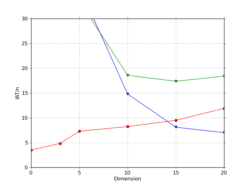
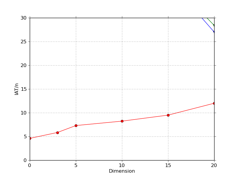
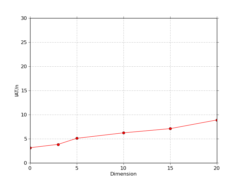
α=0\alpha\geq=0, and 𝑨=𝑷𝚲𝑷𝑨superscript𝑷𝚲𝑷\boldsymbol{A}=\boldsymbol{P}^{\prime}\boldsymbol{\Lambda}\boldsymbol{P}, where 𝚲=diag(λi)𝚲𝑑𝑖𝑎𝑔subscript𝜆𝑖\boldsymbol{\Lambda}=diag(\lambda_{i}). These represent decreasing standard deviations and are increasingly contrasting as α𝛼\alpha increases. More contrasting standard deviations result in further correlated distributions. We consider α=0,5,10,20𝛼051020\alpha=0,5,10,20.

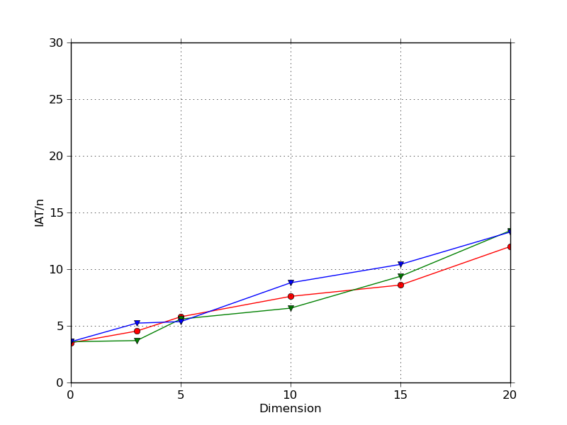
For each combination of n𝑛n and α𝛼\alpha we calculate the Integrated Autocorrelation Time of the resulting chains. Results are shown in Figure 1. Note that the random scan and random direction Gibbs worsen in performance as the σisubscript𝜎𝑖\sigma_{i}’s are more contrasting, our Optimal Direction Gibbs (ODG) remains with an IAT/n12𝑛12n\leq 12. Note that in this general case, the ODG is a random walk; the resulting IAT’s are quite close to the theoretical optimum for an optimal scaled random walk, as explained in (Roberts and Rosenthal, 2001).
Refer to caption Refer to caption
(a) (b)
Refer to caption Refer to caption
(c) (d)
Figure 1: Integrated autocorrelation times divided by the dimension of the MN objective function. Direction gibbs for random scan (blue), random direction (green) and direction according to hsuperscripth^{*} (red). The standard deviations for the MN are set according to (4) for (a) α=0𝛼0\alpha=0 (independent normals) (b) α=5𝛼5\alpha=5, (c) α=10𝛼10\alpha=10 and (d) α=20𝛼20\alpha=20.

3.2 More general objective functions

Suppose then that π(𝒙)𝜋𝒙\pi(\boldsymbol{x}) is the objective distribution of interest with support 𝒳n𝒳superscript𝑛\mathcal{X}\subset\mathbb{R}^{n}. Let 𝑿n𝑿superscript𝑛\boldsymbol{X}\in\mathbb{R}^{n} be a random variable with density π(𝒙)𝜋𝒙\pi(\boldsymbol{x}). Suppose also that for each 𝒙𝒳𝒙𝒳\boldsymbol{x}\in\mathcal{X} we have the Hessian H(𝒙)𝐻𝒙H(\boldsymbol{x}) for logπ()𝜋-\log\pi(\cdot) evaluated at 𝒙𝒙\boldsymbol{x}. By completing the squares in the second order taylor approximation to logπ()𝜋-\log\pi(\cdot), we assume sufficient smoothness such that

logπ(𝒚)C(𝒙)+12(𝒚𝝁(𝒙))H(𝒙)(𝒚𝝁(𝒙)),𝜋𝒚𝐶𝒙12superscript𝒚𝝁𝒙𝐻𝒙𝒚𝝁𝒙-\log\pi(\boldsymbol{y})\approx C(\boldsymbol{x})+\frac{1}{2}(\boldsymbol{y}-\boldsymbol{\mu}(\boldsymbol{x}))^{\prime}H(\boldsymbol{x})(\boldsymbol{y}-\boldsymbol{\mu}(\boldsymbol{x})),

where 𝝁(𝒙)=𝒙H1(𝒙)(𝒙)𝝁𝒙𝒙superscript𝐻1𝒙𝒙\boldsymbol{\mu}(\boldsymbol{x})=\boldsymbol{x}-H^{-1}(\boldsymbol{x})\nabla(\boldsymbol{x}) ((𝒙)𝒙\nabla(\boldsymbol{x}) is the gradient of logπ()𝜋-\log\pi(\cdot) evaluated at 𝒙𝒙\boldsymbol{x}). That is, we have a local MN approximation to π𝜋\pi with mean vector 𝝁(𝒙)𝝁𝒙\boldsymbol{\mu}(\boldsymbol{x}) and precision matrix H(𝒙)𝐻𝒙H(\boldsymbol{x}).

The proposed algorithm runs as follows. At 𝑿(t)=𝒙superscript𝑿𝑡𝒙\boldsymbol{X}^{(t)}=\boldsymbol{x} propose jumping to

𝒀=𝒙+r𝒆𝒀𝒙𝑟𝒆\boldsymbol{Y}=\boldsymbol{x}+r\boldsymbol{e} (5)

where the length r𝑟r\in\mathbb{R} has distribution rN(𝒆H(𝒙)𝒗𝒆H(𝒙)𝒆,𝒆H(𝒙)𝒆)similar-to𝑟𝑁superscript𝒆𝐻𝒙𝒗superscript𝒆𝐻𝒙𝒆superscript𝒆𝐻𝒙𝒆r\sim N\left(-\frac{\boldsymbol{e}^{\prime}H(\boldsymbol{x})\boldsymbol{v}}{\boldsymbol{e}^{\prime}H(\boldsymbol{x})\boldsymbol{e}},\boldsymbol{e}^{\prime}H(\boldsymbol{x})\boldsymbol{e}\right) and 𝒗=𝒙𝝁(𝒙)=𝒙𝒙+H1(𝒙)(𝒙)𝒗𝒙𝝁𝒙𝒙𝒙superscript𝐻1𝒙𝒙\boldsymbol{v}=\boldsymbol{x}-\boldsymbol{\mu}(\boldsymbol{x})=\boldsymbol{x}-\boldsymbol{x}+H^{-1}(\boldsymbol{x})\nabla(\boldsymbol{x}). This translates to

r𝑟\displaystyle r N(𝒆H(𝒙)H1(𝒙)(𝒙)𝒆H(𝒙)𝒆,𝒆H(𝒙)𝒆)similar-toabsent𝑁superscript𝒆𝐻𝒙superscript𝐻1𝒙𝒙superscript𝒆𝐻𝒙𝒆superscript𝒆𝐻𝒙𝒆\displaystyle\sim N\left(-\frac{\boldsymbol{e}^{\prime}H(\boldsymbol{x})H^{-1}(\boldsymbol{x})\nabla(\boldsymbol{x})}{\boldsymbol{e}^{\prime}H(\boldsymbol{x})\boldsymbol{e}},\boldsymbol{e}^{\prime}H(\boldsymbol{x})\boldsymbol{e}\right)
=N(𝒆(𝒙)𝒆H(𝒙)𝒆,𝒆H(𝒙)𝒆).absent𝑁superscript𝒆𝒙superscript𝒆𝐻𝒙𝒆superscript𝒆𝐻𝒙𝒆\displaystyle=N\left(-\frac{\boldsymbol{e}^{\prime}\nabla(\boldsymbol{x})}{\boldsymbol{e}^{\prime}H(\boldsymbol{x})\boldsymbol{e}},\boldsymbol{e}^{\prime}H(\boldsymbol{x})\boldsymbol{e}\right).

As usual, the proposal 𝒀𝒀\boldsymbol{Y} will be accepted with a Metropolis-Hastings probability. In the case that π𝜋\pi is a MN as in Section 2 it is clear that (𝒙)=𝑨(𝒙𝝁)𝒙𝑨𝒙𝝁\nabla(\boldsymbol{x})=\boldsymbol{A}(\boldsymbol{x}-\boldsymbol{\mu}), H(𝒙)=𝑨𝐻𝒙𝑨H(\boldsymbol{x})=\boldsymbol{A}, therefore 𝒗=𝑨1𝑨(𝒙𝝁)𝒗superscript𝑨1𝑨𝒙𝝁\boldsymbol{v}=\boldsymbol{A}^{-1}\boldsymbol{A}(\boldsymbol{x}-\boldsymbol{\mu}) and we are back with the same sampler. The Metropolis-Hasting ratio would be

R=π(𝒚)π(𝒙)q(𝒙|𝒚)q(𝒚|𝒙),𝑅𝜋𝒚𝜋𝒙𝑞conditional𝒙𝒚𝑞conditional𝒚𝒙R=\frac{\pi(\boldsymbol{y})}{\pi(\boldsymbol{x})}\frac{q(\boldsymbol{x}|\boldsymbol{y})}{q(\boldsymbol{y}|\boldsymbol{x})},

where q(|𝒙)=h(𝒆)q𝒆(|𝒙)q(\cdot|\boldsymbol{x})=h^{*}(\boldsymbol{e})q_{\boldsymbol{e}}(\cdot|\boldsymbol{x}) is the density of 𝒀𝒀\boldsymbol{Y} in (5). In Section 2 q𝒆(|𝒙)q_{\boldsymbol{e}}(\cdot|\boldsymbol{x}) is the conditional distribution over the direction 𝒆𝒆\boldsymbol{e}, given 𝒙𝒙\boldsymbol{x} (gibbs kernel), and cancels out with π(𝒙)𝜋𝒙\pi(\boldsymbol{x}) (h(𝒆)superscript𝒆h^{*}(\boldsymbol{e}) would cancel out with h(𝒆)superscript𝒆h^{*}(-\boldsymbol{e}) since the Hessian is constant; H(𝒙)=𝑨𝐻𝒙𝑨H(\boldsymbol{x})=\boldsymbol{A}). Let g(𝒙)=logπ(𝒙)𝑔𝒙𝜋𝒙g(\boldsymbol{x})=\log\pi(\boldsymbol{x}), then

logR=(g(𝒚)+logq(𝒙|𝒚))(g(𝒙)+logq(𝒚|𝒙)).𝑅𝑔𝒚𝑞conditional𝒙𝒚𝑔𝒙𝑞conditional𝒚𝒙\log R=(g(\boldsymbol{y})+\log q(\boldsymbol{x}|\boldsymbol{y}))-(g(\boldsymbol{x})+\log q(\boldsymbol{y}|\boldsymbol{x})).

Let

ψ𝒙(𝒆,r)=g(𝒙)+logq(𝒙+r𝒆|𝒙).subscript𝜓𝒙𝒆𝑟𝑔𝒙𝑞𝒙conditional𝑟𝒆𝒙\psi_{\boldsymbol{x}}(\boldsymbol{e},r)=g(\boldsymbol{x})+\log q(\boldsymbol{x}+r\boldsymbol{e}|\boldsymbol{x}).

Note that q(𝒙+r𝒆|𝒙)=h(𝒆)q𝒆(𝒙+r𝒆|𝒙)𝑞𝒙conditional𝑟𝒆𝒙superscript𝒆subscript𝑞𝒆𝒙conditional𝑟𝒆𝒙q(\boldsymbol{x}+r\boldsymbol{e}|\boldsymbol{x})=h^{*}(\boldsymbol{e})q_{\boldsymbol{e}}(\boldsymbol{x}+r\boldsymbol{e}|\boldsymbol{x}) and therefore

q(𝒙+r𝒆|𝒙)𝑞𝒙conditional𝑟𝒆𝒙\displaystyle q(\boldsymbol{x}+r\boldsymbol{e}|\boldsymbol{x}) =KH(𝒙)(𝒆H(𝒙)𝒆)12(𝒆H(𝒙)𝒆)122πabsentsubscript𝐾𝐻𝒙superscriptsuperscript𝒆𝐻𝒙𝒆12superscriptsuperscript𝒆𝐻𝒙𝒆122𝜋\displaystyle=K_{H(\boldsymbol{x})}(\boldsymbol{e}^{\prime}H(\boldsymbol{x})\boldsymbol{e})^{-{1\over 2}}\frac{(\boldsymbol{e}^{\prime}H(\boldsymbol{x})\boldsymbol{e})^{1\over 2}}{\sqrt{2\pi}}
exp{𝒆H(𝒙)𝒆2(r+𝒆(𝒙)𝒆H(𝒙)𝒆)2},absentsuperscript𝒆𝐻𝒙𝒆2superscript𝑟superscript𝒆𝒙superscript𝒆𝐻𝒙𝒆2\displaystyle\quad\cdot\exp\left\{-\frac{\boldsymbol{e}^{\prime}H(\boldsymbol{x})\boldsymbol{e}}{2}\left(r+\frac{\boldsymbol{e}^{\prime}\nabla(\boldsymbol{x})}{\boldsymbol{e}^{\prime}H(\boldsymbol{x})\boldsymbol{e}}\right)^{2}\right\},

and

ψ𝒙(𝒆,r)=g(𝒙)+logKH(𝒙)𝒆H(𝒙)𝒆2(r+𝒆(𝒙)𝒆H(𝒙)𝒆)2,subscript𝜓𝒙𝒆𝑟𝑔𝒙subscript𝐾𝐻𝒙superscript𝒆𝐻𝒙𝒆2superscript𝑟superscript𝒆𝒙superscript𝒆𝐻𝒙𝒆2\psi_{\boldsymbol{x}}(\boldsymbol{e},r)=g(\boldsymbol{x})+\log K_{H(\boldsymbol{x})}-\frac{\boldsymbol{e}^{\prime}H(\boldsymbol{x})\boldsymbol{e}}{2}\left(r+\frac{\boldsymbol{e}^{\prime}\nabla(\boldsymbol{x})}{\boldsymbol{e}^{\prime}H(\boldsymbol{x})\boldsymbol{e}}\right)^{2},

where

KH(𝒙)1=𝒆=1(𝒆H(𝒙)𝒆)12𝑑𝒆superscriptsubscript𝐾𝐻𝒙1subscriptnorm𝒆1superscriptsuperscript𝒆𝐻𝒙𝒆12differential-d𝒆K_{H(\boldsymbol{x})}^{-1}=\int_{||\boldsymbol{e}||=1}(\boldsymbol{e}^{\prime}H(\boldsymbol{x})\boldsymbol{e})^{-{1\over 2}}d\boldsymbol{e}

is the normalizing constant of hsuperscripth^{*} that now depends on 𝒙𝒙\boldsymbol{x}. We then have

R(𝒙,𝒆,r)=exp{ψ𝒙+r𝒆(𝒆,r)ψ𝒙(𝒆,r)}.𝑅𝒙𝒆𝑟subscript𝜓𝒙𝑟𝒆𝒆𝑟subscript𝜓𝒙𝒆𝑟R(\boldsymbol{x},\boldsymbol{e},r)=\exp\{\psi_{\boldsymbol{x}+r\boldsymbol{e}}(-\boldsymbol{e},r)-\psi_{\boldsymbol{x}}(\boldsymbol{e},r)\}. (6)

Therefore, the probability of accepting a jump from 𝒙𝒙\boldsymbol{x} to 𝒚=𝒙+r𝒆𝒚𝒙𝑟𝒆\boldsymbol{y}=\boldsymbol{x}+r\boldsymbol{e} should be min{1,R(𝒙,𝒆,r)}1𝑅𝒙𝒆𝑟\min\{1,R(\boldsymbol{x},\boldsymbol{e},r)\}. However, it is not possible to obtain KH(𝒙)subscript𝐾𝐻𝒙K_{H(\boldsymbol{x})} analytically. For dimension n=2𝑛2n=2 we calculate KH(𝒙)subscript𝐾𝐻𝒙K_{H(\boldsymbol{x})} numerically, only for comparison purposes.

An alternative distribution of directions would be the following. Assuming that 𝑨=H(𝒙)𝑨𝐻𝒙\boldsymbol{A}=H(\boldsymbol{x}) is positive defined, we can use its eigenvalues and eigenvectors. We will take the directions 𝒆𝒆\boldsymbol{e} as the eigenvectors of matrix H(𝒙)𝐻𝒙H(\boldsymbol{x}), so 𝒆{𝒆1,𝒆2,,𝒆n}𝒆subscript𝒆1subscript𝒆2subscript𝒆𝑛\boldsymbol{e}\in\{\boldsymbol{e}_{1},\boldsymbol{e}_{2},\ldots,\boldsymbol{e}_{n}\}. The i𝑖i-th direction will be selected with probability proportional to λi1superscriptsubscript𝜆𝑖1\lambda_{i}^{-1}, where λisubscript𝜆𝑖\lambda_{i} is the eigenvalue corresponding to the i𝑖i-th eigenvector , i=1,2,,n𝑖12𝑛i=1,2,\ldots,n . Then h1(𝒆i)=(kλi)1subscript1subscript𝒆𝑖superscript𝑘subscript𝜆𝑖1h_{1}(\boldsymbol{e}_{i})=\left(k\lambda_{i}\right)^{-1}, where k=i=1nλi1𝑘superscriptsubscript𝑖1𝑛superscriptsubscript𝜆𝑖1k=\sum_{i=1}^{n}\lambda_{i}^{-1}. By doing this the distribution of 𝐞𝐞\mathbf{e} becomes discrete. Moreover, we avoid the problem we have with de normalization constant KH(𝒆)subscript𝐾𝐻𝒆K_{H(\boldsymbol{e})} and the implementation can be done for large values of dimension n𝑛n.

It Iis easy to see that direction 𝐞1subscript𝐞1\mathbf{e}_{1}, corresponding to the lowest eigenvalue λnsubscript𝜆𝑛\lambda_{n} of H(𝒙)𝐻𝒙H(\boldsymbol{x}), is optimal indeed. Note that

min𝒆=1I𝒆(𝑿(t+1),𝑿(t))subscriptnorm𝒆1subscript𝐼𝒆superscript𝑿𝑡1superscript𝑿𝑡\displaystyle\min_{\|\boldsymbol{e}\|=1}I_{\boldsymbol{e}}\left(\boldsymbol{X}^{(t+1)},\boldsymbol{X}^{(t)}\right) =min𝒆=1{C+12log(𝒆H(𝒙)𝒆)}absentsubscriptnorm𝒆1𝐶12superscript𝒆𝐻𝒙𝒆\displaystyle=\min_{\|\boldsymbol{e}\|=1}\left\{C+\dfrac{1}{2}\log\left(\boldsymbol{e}^{\prime}H(\boldsymbol{x})\boldsymbol{e}\right)\right\}
=C+12log(min𝒆=1{𝒆H(𝒙)𝒆})=C+12logλ1.absent𝐶12subscriptnorm𝒆1superscript𝒆𝐻𝒙𝒆𝐶12subscript𝜆1\displaystyle=C+\dfrac{1}{2}\log\left(\min_{\|\boldsymbol{e}\|=1}\left\{\boldsymbol{e}^{\prime}H(\boldsymbol{x})\boldsymbol{e}\right\}\right)=C+\dfrac{1}{2}\log\lambda_{1}.

The minimum is reached when 𝒆=𝒆1𝒆subscript𝒆1\boldsymbol{e}=\boldsymbol{e}_{1}, the eigenvector associated to λ1subscript𝜆1\lambda_{1}.

3.3 Example: The skew-normal distribution

To test the performance of our algorithm we will use as objective distribution a variant of the skew-normal distribution. We choose this distribution due its simplicity and versatility, plus the fact that it allows us to calculate analytically the gradient and the Hessian of logπ𝜋-\log\pi.

The multivariate skew-normal probability density function is given by

f(𝒚)=2ϕn(𝒚𝝃;𝚺)Φ(𝜶(𝒚𝝃)),𝑓𝒚2subscriptitalic-ϕ𝑛𝒚𝝃𝚺Φsuperscript𝜶𝒚𝝃f(\boldsymbol{y})=2\phi_{n}(\boldsymbol{y}-\boldsymbol{\xi};\boldsymbol{\Sigma})\Phi(\boldsymbol{\alpha}^{\prime}(\boldsymbol{y}-\boldsymbol{\xi})),

where ϕn(;𝚺)subscriptitalic-ϕ𝑛𝚺\phi_{n}(\cdot;\boldsymbol{\Sigma}) is the multivariate normal probability density function with mean vector 𝟎0\mathbf{0} and variance-covariance matrix 𝚺𝚺\boldsymbol{\Sigma}, Φ()Φ\Phi(\cdot) is the standard univariate normal cumulative distribution function, 𝝃𝝃\boldsymbol{\xi} is a localization parameter and 𝜶𝜶\boldsymbol{\alpha} is a shape parameter (Azzalini and Adelchi, 2005).

Φ()Φ\Phi(\cdot) is called perturbation function and may be the cumulative distribution function of any univariate symmetric distribution around 00. In our case, we are going to use the Logistic cumulative distribution function with mean 00 and scale parameter s=3π𝑠3𝜋s=\frac{\sqrt{3}}{\pi}, which is

G(x)=11+exp{πx/3}.𝐺𝑥11𝜋𝑥3G(x)=\dfrac{1}{1+\exp\left\{-\pi x/\sqrt{3}\right\}}.
Refer to caption Refer to caption
a) b)
Refer to caption Refer to caption
c) d)
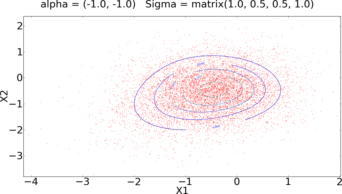
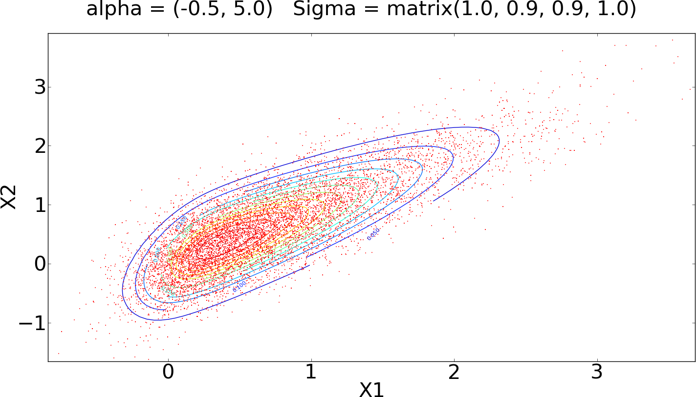
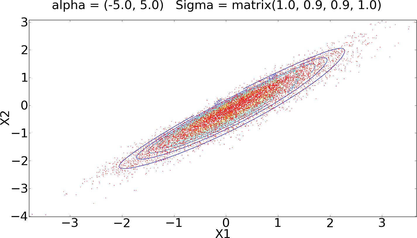
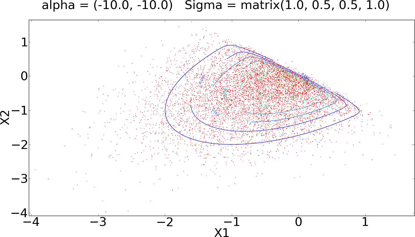
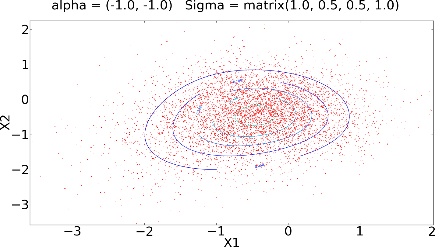
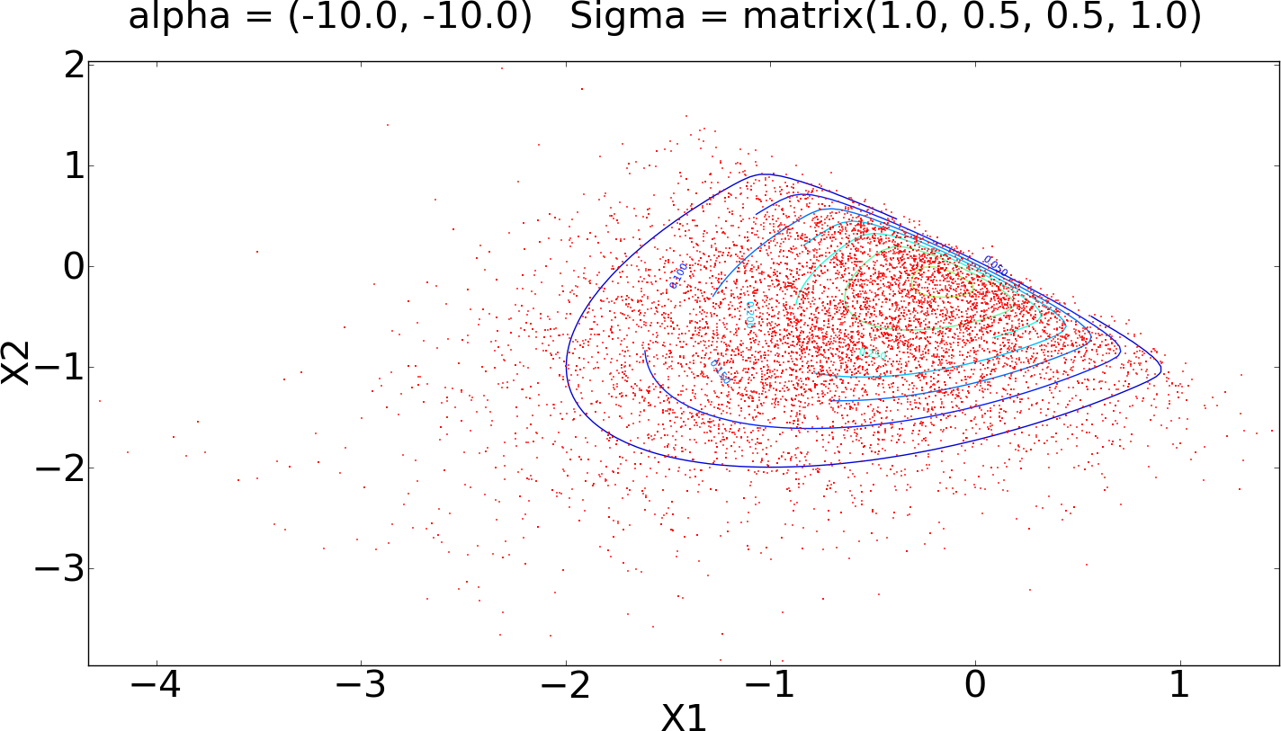
Figure 2: Simulations obtained with the Optimal Direction Gibbs algorithm using distribution hh*.
𝜶𝜶\boldsymbol{\alpha} 𝚺𝚺\boldsymbol{\Sigma} IAT Acceptance rate
a) (1.0,1.0)1.01.0(-1.0,-1.0) (1.0,0.5,0.5,1.0)1.00.50.51.0(1.0,0.5,0.5,1.0) 4.0398704.0398704.039870 0.87120.87120.8712
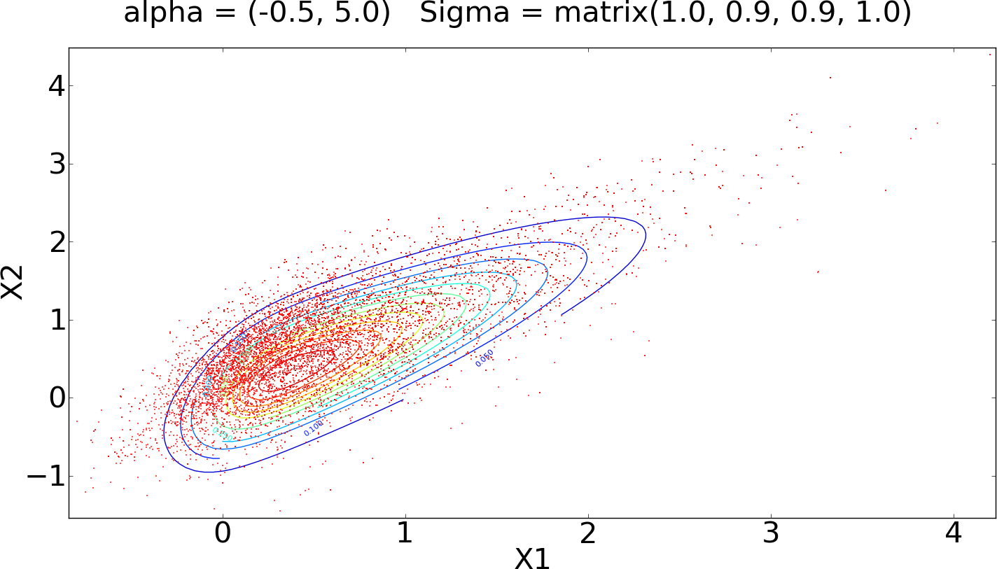
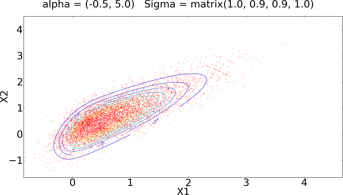
b) (0.5,5.0)0.55.0(-0.5,5.0) (1.0,0.9,0.9,1.0)1.00.90.91.0(1.0,0.9,0.9,1.0) 6.9449006.9449006.944900 0.76930.76930.7693
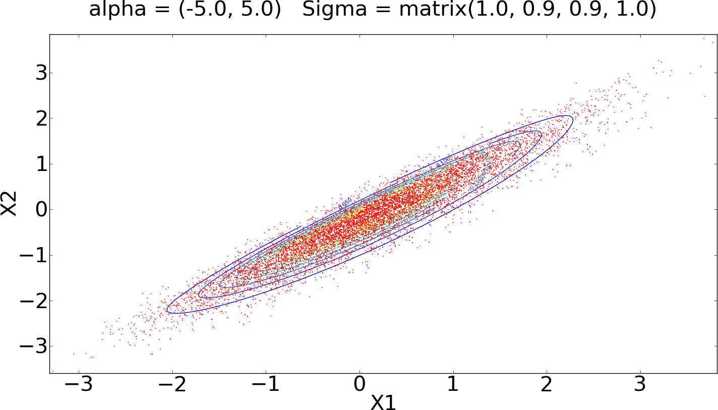
c) (5.0,5.0)5.05.0(-5.0,5.0) (1.0,0.9,0.9,1.0)1.00.90.91.0(1.0,0.9,0.9,1.0) 3.9098963.9098963.909896 0.84850.84850.8485
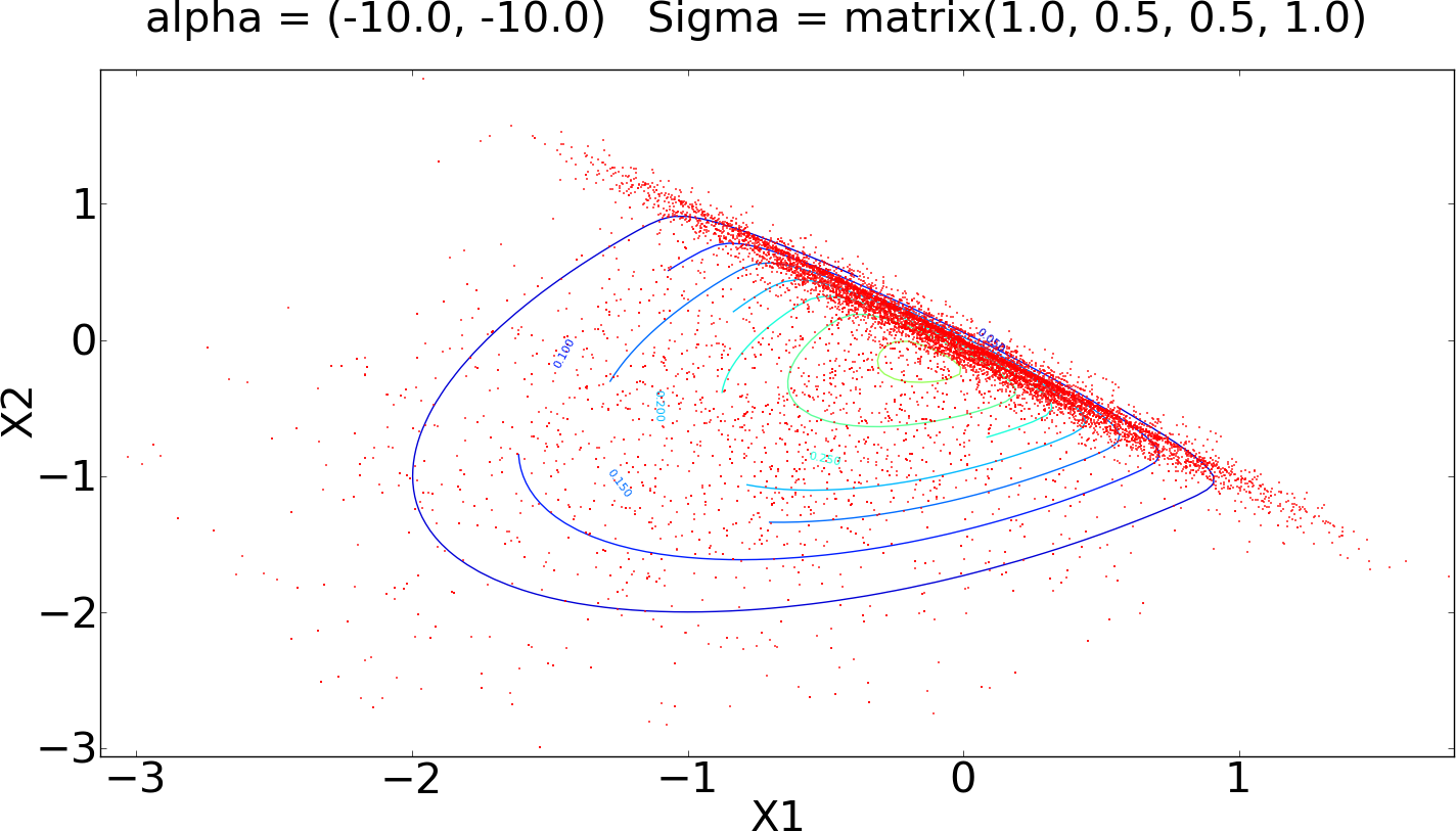
d) (10.0,10.0)10.010.0(-10.0,-10.0) (1.0,0.5,0.5,1.0)1.00.50.51.0(1.0,0.5,0.5,1.0) 7.6292537.6292537.629253 0.68920.68920.6892
Table 1: Acceptance rate and IAT for simulations obtained with the Optimal Direction Gibbs algorithm using distribution hh*.

Then, the density function of our objective distribution is given by

π(𝒙)=2(|A|(2π)n)1/2exp{12𝒙𝑨𝒙}11+exp{π𝜶𝒙/3},𝜋𝒙2superscript𝐴superscript2𝜋𝑛1212superscript𝒙𝑨𝒙11𝜋superscript𝜶𝒙3\pi(\boldsymbol{x})=2\left(\dfrac{|A|}{(2\pi)^{n}}\right)^{1/2}\exp\left\{-\dfrac{1}{2}\boldsymbol{x}^{\prime}\boldsymbol{A}\boldsymbol{x}\right\}\dfrac{1}{1+\exp\left\{-\pi\boldsymbol{\alpha}^{\prime}\boldsymbol{x}/\sqrt{3}\right\}},

where 𝑨=𝚺1𝑨superscript𝚺1\boldsymbol{A}=\boldsymbol{\Sigma}^{-1}. In order to implement the algorithm we need to calculate the gradient and Hessian of logπ(𝒙)𝜋𝒙-\log\pi(\boldsymbol{x}). It is easy to see that

(𝒙)=𝑨𝒙(1G(𝜶𝒙))𝜶,𝒙𝑨𝒙1𝐺superscript𝜶𝒙𝜶\nabla(\boldsymbol{x})=\boldsymbol{A}\boldsymbol{x}-\left(1-G(\boldsymbol{\alpha}^{\prime}\boldsymbol{x})\right)\boldsymbol{\alpha},

and

H(𝒙)=A+g(𝜶𝒙)𝜶𝜶,𝐻𝒙𝐴𝑔superscript𝜶𝒙𝜶superscript𝜶\displaystyle H(\boldsymbol{x})=A+g(\boldsymbol{\alpha}^{\prime}\boldsymbol{x})\boldsymbol{\alpha}\boldsymbol{\alpha}^{\prime},

where g()𝑔g(\cdot) is the Logistic probability density function.

To test the algorithm we consider the case n=2𝑛2n=2. Figure 2 shows the contour plots of the objective distribution for different values of 𝚺𝚺\boldsymbol{\Sigma} and 𝜶𝜶\boldsymbol{\alpha}. It also shows the simulations obtained using the algorithm with distribution hsuperscripth^{*}, after 10,0001000010,000 iterations. We set the initial point 𝑿(0)=𝟎superscript𝑿00\boldsymbol{X}^{(0)}=\mathbf{0} and the burn in is not needed. Table 1 shows the acceptance rate and IAT for each example. Note that the value of the IAT is small and the acceptance rate is large in all cases. Both measures indicate that the performance of the algorithm is quite good. Is important to mention that a conventional Gibbs sampler cannot be used for this example since the full conditional distributions do not have any close form. Our scheme has not that kind of difficulties.

Unfortunately, the implementation is not as simple for dimension n3𝑛3n\geq 3 since we need to calculate the normalization constant KH(𝒙)subscript𝐾𝐻𝒙K_{H(\boldsymbol{x})} numerically.

Refer to caption Refer to caption
a) b)
Refer to caption Refer to caption
c) d)
Figure 3: Simulations obtained with the Optimal Direction Gibbs algorithm using distribution h1subscript1h_{1}.

In Subsection 3.2 we proposed an alternative direction distribution h1subscript1h_{1} to avoid calculating KH(𝒙)subscript𝐾𝐻𝒙K_{H(\boldsymbol{x})}. We test the algorithm using this distribution on the same examples. Figure 3 shows some very interesting results. Simulations in examples a) and b) are well distributed over the region of interest. However, in examples c) and d) simulations are concentrated in a specific region. This results from the fact that the eigenvalues of H(𝒙)𝐻𝒙H(\boldsymbol{x}) are very contrasting, one is much larger than the other, and consequently, simulations are obtained in similar directions constantly.

This suggests that the scheme works well in simple cases, but it becomes inefficient against more skewed distributions. However, we can still modify h1subscript1h_{1}. We take the directions 𝒆𝒆\boldsymbol{e} as eigenvectors of H(𝒙)𝐻𝒙H(\boldsymbol{x}), but the probability of choosing 𝒆isubscript𝒆𝑖\boldsymbol{e}_{i} will now be proportional to (λi)bsuperscriptsubscript𝜆𝑖𝑏\left(\lambda_{i}\right)^{-b}, where bBeta(1,9)similar-to𝑏𝐵𝑒𝑡𝑎19b\sim Beta(1,9), this is h2(𝒆i)(λi)bproportional-tosubscript2subscript𝒆𝑖superscriptsubscript𝜆𝑖𝑏h_{2}(\boldsymbol{e}_{i})\propto\left(\lambda_{i}\right)^{-b}. By doing this we allow the chance that probabilities become more balanced in regions where there is a very dominant eigenvalue.
Refer to caption Refer to caption
a) b)
Refer to caption Refer to caption
c) d)
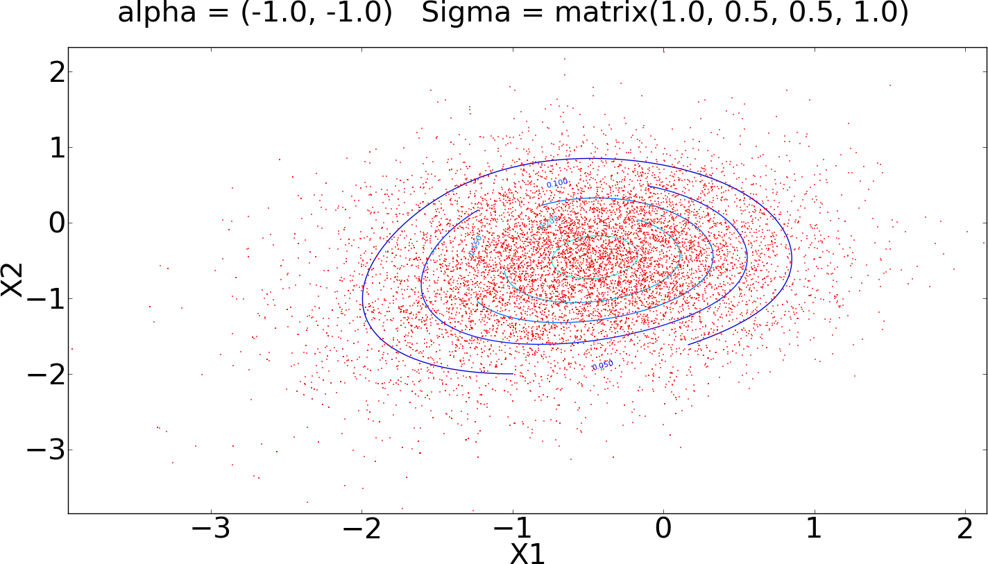
Figure 4: Simulations obtained with the Optimal Direction Gibbs algorithm using distribution h2subscript2h_{2}.

Figure 4 shows the behaviour of the resulting algorithm. Examples a) and b) show a good performance as before. On the other hand, examples c) and d), which we identified as difficult above, seem to have been corrected. Table 2 shows the acceptance rate and IAT. Here we see good results. Acceptance rates remain high and do not represent a problem. The IAT is slightly higher than in Table 1, except by example c); however, the difference is not quite significant.

𝜶𝜶\boldsymbol{\alpha} 𝚺𝚺\boldsymbol{\Sigma} IAT Acceptance rate
a) (1.0,1.0)1.01.0(-1.0,-1.0) (1.0,0.5,0.5,1.0)1.00.50.51.0(1.0,0.5,0.5,1.0) 4.4973014.4973014.497301 0.87930.87930.8793
b) (0.5,5.0)0.55.0(-0.5,5.0) (1.0,0.9,0.9,1.0)1.00.90.91.0(1.0,0.9,0.9,1.0) 7.8446307.8446307.844630 0.75340.75340.7534
c) (5.0,5.0)5.05.0(-5.0,5.0) (1.0,0.9,0.9,1.0)1.00.90.91.0(1.0,0.9,0.9,1.0) 2.7054162.7054162.705416 0.88090.88090.8809
d) (10.0,10.0)10.010.0(-10.0,-10.0) (1.0,0.5,0.5,1.0)1.00.50.51.0(1.0,0.5,0.5,1.0) 8.8214708.8214708.821470 0.73270.73270.7327
Table 2: Acceptance rate and IAT for simulations obtained with the Optimal Direction Gibbs algorithm using distribution h2subscript2h_{2}.

Direction distribution h2subscript2h_{2} seems a good alternative for our optimal direction distribution since it shows good performance and the IAT values are very similar to those obtained with our original scheme. The parameters of the Beta distribution were selected intuitively. In fact, those parameters allows us to change distribution h2subscript2h_{2} in order to get better results.

4 Discussion

Our Optimal Direction Gibbs sampler presents interesting characteristics in examples where either a conventional gibbs sampler is impossible to implement or o ther MCMC methods (eg. a Random Walk Metropolis-Hastings) would be vey difficult to tune. The truncated normal example is of great relevance in the field of inverse problems and we have also worked with strongly skewed distributions with contrasting scales, with promising results in all cases.

5 Acknowledgements

DAPR and MSC thank CONACyT for a MSc scholarship since part of this work was conducted while finishing their MSc studies at CIMAT. Part of JAC work was founded by CONACyT grant 128477.

References

  • Azzalini and Adelchi (2005) Azzalini, Adelchi (2005) The skew-normal distribution and related multivariate families. Scandinavian Journal of Statistics 2:159–188
  • Kaufman and Smith (1994) Kaufman D, Smith R (1994) Direction choice for accelerated convergence in hit-and-run sampling. Operation Research 46(1):84–95
  • Roberts and Rosenthal (2001) Roberts GO, Rosenthal JS (2001) Optimal scaling for various metropolis-hastings algorithms. Statistical Science 16(4):351–367