Optimal Weights Mixed Filter for Removing Mixture of Gaussian and Impulse Noises

Abstract

According to the character of Gaussian, we modify the Rank-Ordered Absolute Differences (ROAD) to Rank-Ordered Absolute Differences of mixture of Gaussian and impulse noises (ROADG). It will be more effective to detect impulse noise when the impulse is mixed with Gaussian noise. Combining rightly the ROADG with Optimal Weights Filter (OWF), we obtain a new method to deal with the mixed noise, called Optimal Weights Mixed Filter (OWMF). The simulation results show that the method is effective to remove the mixed noise.

1 Introduction

Noise can be systematically introduced into digitized images during acquisition and transmission, which usually degrade the quality of digitized images. However, various image-related applications, such as aerospace, medical image analysis, object detection etc., generally require effective noise suppression to produce reliable results. The problem of noise removal from a digitized image is one of the most important ones in digital image processing. The nature of the problem depends on the type of noise to the image. Generally, two noise models can adequately represent most noise added to images. Often in practice it is assumed that the noise has two components: an additive Gaussian noise and an impulse noise.

The additive Gaussian noise model is:

$$Y(x)=f(x)+\epsilon(x),\;x\in\mathbf{I,}$$ (1)

where $\mathbf{I}=\{\frac{1}{N},\frac{2}{N},\cdots,\frac{N-1}{N},1\}^{2},$ $N\in\mathbf{N}$, $Y$ is the observed image brightness, $f:\mathbf{I}\mapsto[c,d]$ is an unknown target regression function, and $\epsilon(x),$ $x\in\mathbf{I,}$ are independent and identically distributed (i.i.d.) Gaussian random variables with mean $0$ and standard deviation $\sigma>0.$ The additive Gaussian noise is characterized by adding to each digitized image pixel a value from a zero-mean Gaussian distribution. Such noise is usually introduced during image acquisition. The zero-mean property of this Gaussian distribution makes it possible to remove the Gaussian noise by Non-Local weighted averaging. Important denoising methods for the Gaussian noise model have been well developed in recent years, see for example Polzehl and Spokoiny (2000), Buades et al. (2005), Kervrann and Boulanger (2006), Aharon et al. (2006), Dabov et al. (2007), Cai et al. (2008), Hammond and Simoncelli (2008), Lou et al. (2010), Katkovnik et al. (2010), and Jin et al. (2011).

The random impulse noise model is: for $x\in\mathbf{I,}$

$$Y\left(x\right)=\left\{\begin{array}[]{ll}n(x),&\text{if }x\in\mathbf{B},\\ f(x),&\text{if }x\in\mathbf{I}\backslash\mathbf{B},\end{array}\right.$$ (2)

where $\mathbf{B}$ is the set of pixels contaminated by impulse noise, $\mathbb{P}(\mathbf{B})=p$ is the impulse probability (the proportion of the occurrence of the impulse noise), $n(x)$ are independent random variables uniformly distributed on some interval $[c,d]$. The impulse noise is characterized by replacing a portion of an image’s pixel values with random values, leaving the remaining one unchanged. Such a noise can be introduced due to transmission errors, malfunctioning pixel elements in the camera sensors, faulty memory locations, and timing errors in analog-to-digital conversion. Recently, some important methods have been proposed to remove the impulse noise, see for example: Hwang and Haddad (1995), Abreu et al. (1996), Chen and Wu (2001b), Chan et al. (2004), Nikolova (2004), Wenbin (2005), Dong et al. (2007), and Yu et al. (2008),

To remove a mixture of the Gaussian and impulse noises which defined by

$$Y\left(x\right)=\left\{\begin{array}[]{ll}n(x),&\text{if }x\in\mathbf{B},\\ f(x)+\epsilon(x),&\text{if }x\in\mathbf{I}\backslash\mathbf{B},\end{array}\right.$$ (3)

the above mentioned methods are not effective: the Gaussian noise removal methods cannot adequately remove impulse noise, for they interpret the impulse noise pixel as edges to be preserved; when impulse removal methods are applied to an image corrupted with the Gaussian noise, such filters, in practice, leave grainy, visually disappointing results. Garnett et al. (2005) introduced a new local image statistic called Rank Ordered Absolute Difference (ROAD) to identify the impulse noisy pixels and incorporated it into a filter designed to remove the additive Gaussian noise. As a result they have obtained a trilateral filter capable to remove mixed Gaussian and impulse noise. This method also performs well for removing the single impulse noise. For other developpements in this direction we refer to Bouboulis et al. (2010), Li et al. (2010), Xiao et al. (2011)), Luisier et al. (2011).

In this paper, we propose a new filter that we call Optimal Weights Mixed Filter (OWMF). The idea of our method come from the combination of the ROAD statistic of Garnett et al. (2005) and the Optimal Weights Filter in Jin et al. (2011). In the paper, we modify the Rank-Ordered Absolute Differences (ROAD) to Rank-Ordered Absolute Differences of mixture of Gaussian and impulse noises (ROADG). It will be more effective to detect impulse noise when the impulse is mixed with Gaussian noise. The ROADG statistic will give a weight for all pixels in the image, which take value in the interval $(0,1]$. The weight will get low value (the value may be near to 0) when a pixel is contaminated by impulse noise; otherwise, the weight will carry a high value (the value may be near to 1). Then the Optimal Weights Filter (OWF) combining with the ROADG statistic can detect the impulse points in the image and give the proper weights to deal with the mixed noise. As a result, we obtain our new filter. The simulation results show that the proposed filter can effectively remove the mixture of impulse noise and the Gaussian noise. Moreover, when applied to either the single impulse noise or the single Gaussian noise it performs as good as the best filters specialized to single noises.

The rest of the paper is organized as follows. In Section 2 after a short recall of the Optimal Weights Filter and a brief presentation of the Trilateral Filter whose main ideas will be used in the definition of our new filter, we introduce our filter. In section 3, we provide visual examples and numerical results that demonstrate our method’s soundness. Section 4 is a brief conclusion.

2 Algorithms

2.1 Optimal Weights Filter

For any pixel $x_{0}\in\mathbf{I}$ and a given $h>0,$ the square window of pixels

$$\mathbf{U}_{x_{0},h}=\left\{x\in\mathbf{I}:\|x-x_{0}\|_{\infty}\leq h\right\}$$ (4)

will be called search window at $x_{0}$, where $h$ is a positive integer. The size of the square search window $\mathbf{U}_{x_{0},h}$ is the positive integer number $M=(2h+1)^{2}=\mathrm{card\ }\mathbf{U}_{x_{0},h}.$ For any pixel $x\in\mathbf{U}_{x_{0},h}$ and a given integer $\eta>0$ a second square window of pixels

$$\mathbf{V}_{x,\eta}=\left\{y\in\mathbf{I}:\|y-x\|_{\infty}\leq\eta\right\}$$ (5)

will be called for short a patch window at $x$ in order to be distinguished from the search window $\mathbf{U}_{x_{0},h}.$ The size of the patch window $\mathbf{V}_{x,\eta}$ is the positive integer $m=(2\eta+1)^{2}=\mathrm{card\ }\mathbf{V}_{x_{0},\eta}.$ The vector $\mathbf{Y}_{x,\eta}=\left(Y\left(y\right)\right)_{y\in\mathbf{V}_{x,\eta}}$ formed by the values of the observed noisy image $Y$ at pixels in the patch $\mathbf{V}_{x,\eta}$ will be called simply data patch at $x\in\mathbf{U}_{x_{0},h}.$ For any $x_{0}\in\mathbf{I}$ and any $x\in\mathbf{U}_{x_{0},h}$, a distance between the data patches $\mathbf{Y}_{x,\eta}=\left(Y\left(y\right)\right)_{y\in\mathbf{V}_{x,\eta}}$ and $\mathbf{Y}_{x_{0},\eta}=\left(Y\left(y\right)\right)_{y\in\mathbf{V}_{x_{0},\eta}}$ is defined by

$$\mathbf{d}^{2}\left(\mathbf{Y}_{x,\eta},\mathbf{Y}_{x_{0},\eta}\right)=\frac{1}{m}\left\|\mathbf{Y}_{x,\eta}-\mathbf{Y}_{x_{0},\eta}\right\|_{2}^{2},$$ (6)

where

$$\left\|\mathbf{Y}_{x,\eta}-\mathbf{Y}_{x_{0},\eta}\right\|_{2}^{2}=\sum\limits_{y\in\mathbf{V}_{x_{0},\eta}}(Y(T_{x}y)-Y(y))^{2}$$

and $T_{x}$ is the translation mapping: $T_{x}y=x+(y-x_{0})$. As

$$Y(T_{x}y)-Y(y)=f(T_{x}y)-f(y)+\epsilon(T_{x}y)-\epsilon(y)$$

we have

$$\mathbb{E}(Y(T_{x}y)-Y(y))^{2}=(f(T_{x}y)-f(y))^{2}+2\sigma^{2}.$$

If we use the approximation

$$(f(T_{x}y)-f(y))^{2}\approx(f(x)-f(x_{0}))^{2}=\rho_{f,x_{0}}^{2}(x)$$

and the law of large numbers, it seems reasonable that

$$\rho_{f,x_{0}}^{2}(x)\approx\mathbf{d}^{2}(\mathbf{Y}_{x,\eta}-\mathbf{Y}_{x_{0},\eta})-2\sigma^{2}.$$

As shown in (Jin et al., 2011), in practice, a much better denoising results are obtained by using the following approximation

$$\rho_{f,x_{0}}(x)\approx\widehat{\rho}_{x_{0}}(x)=\left(d(\mathbf{Y}_{x,\eta}-\mathbf{Y}_{x_{0},\eta})-\sqrt{2}\sigma\right)^{+}.$$ (7)

The fact that $\widehat{\rho}_{x_{0}}(x)$ is a good estimator of $\rho_{f,x_{0}}$ was justified by the convergence results in (Jin et al., 2011) (cf. Theorems 3 and 4 of (Jin et al., 2011)). The Optimal Weights Filter is defined by

$$\mbox{OWF}(f)(x_{0})=\frac{\sum\limits_{x\in\mathbf{U}_{x_{0},h}}\kappa_{\text{tr}}(\frac{\widehat{\rho}_{x_{0}}\left(x\right)}{\widehat{a}})Y(x)}{\sum\limits_{y\in\mathbf{U}_{x_{0},h}}\kappa_{\text{tr}}(\frac{\widehat{\rho}_{x_{0}}\left(x\right)}{\widehat{a}})},$$ (8)

where $\kappa_{\text{tr}}$ is the usual triangular kernel:

$$\kappa_{\text{tr}}\left(t\right)=\left(1-\left|t\right|\right)^{+},\quad t\in\mathbf{R}^{1}.$$ (9)

Remark 1

The bandwidth $\widehat{a}>0$ is the solution of

$$\sum_{x\in\mathbf{U}_{x_{0},h}}\widehat{\rho}_{x_{0}}(x)(\widehat{a}-\widehat{\rho}_{x_{0}}(x))^{+}=\sigma^{2},$$

and can be calculated as follows. We sort the set $\{\widehat{\rho}_{x_{0}}(x):x\in\mathbf{U}_{x_{0},h}\}$ in the ascending order $0=\widehat{\rho}_{x_{0}}(x_{1})\leq\widehat{\rho}_{x_{0}}(x_{2})\leq\cdots\leq\widehat{\rho}_{x_{0}}(x_{M})<\widehat{\rho}_{x_{0}}(x_{M+1})=+\infty$, where $M=\mathrm{card}\,\mathbf{U}_{x_{0},h}$. Let

$$a_{k}=\frac{\sigma^{2}+\sum\limits_{i=1}^{k}\widehat{\rho}_{x_{0}}(x_{i})^{2}}{\sum\limits_{i=1}^{k}\widehat{\rho}_{x_{0}}(x_{i})},\quad 1\leq k\leq M,$$ (10)

and

$$k^{\ast} = \max\{1\leq k\leq M\,:\,a_{k}\geq\widehat{\rho}_{x_{0}}(x_{k})\}$$ (11)

$$= \min\{1\leq k\leq M\,:\,a_{k}<\widehat{\rho}_{x_{0}}(x_{k})\}-1,$$

with the convention that $a_{k}=\infty$ if $\widehat{\rho}_{x_{0}}(x_{k})=0$ and that $\min\varnothing=M+1$. The solution can be expressed as $\widehat{a}=a_{k^{\ast}}$; moreover, $k^{\ast}$ is the unique integer $k\in\{1,\cdots,M\}$ such that $a_{k}\geq\widehat{\rho}_{x_{0}}(x_{k})$ and $a_{k+1}<\widehat{\rho}_{x_{0}}(x_{k+1})$ if $k<M$.

The proof of Remark 1 can be found in (Jin et al., 2011).

2.2 ROAD statistic and Trilateral Filter

In (Garnett et al., 2005), Garnett et al introduced the Rank-Ordered Absolute Differences (ROAD) statistic to detect points contaminated by impulse noise. For any pixel $x_{0}\in\mathbf{I}$ and a given $d>0,$ we define the square window of pixels

$$\Omega_{x_{0},d}^{0}=\{x:0<N\|x-x_{0}\|_{\infty}\leq d\},$$

where $d$ is a positive integer. The square window will be called deleted neighborhood at $x_{0}$. The ROAD statistic is defined by

$$ROAD(x_{0})=\sum_{i=1}^{K}r_{i}(x_{0}),\text{ }x_{0}\in\mathbf{I},$$ (12)

where $r_{i}(x_{0})$ is the $i$-th smallest term in the set $\{|Y(x)-Y(x_{0})|:x\in\Omega_{x_{0},d}^{0}\}$ and $2\leq K<\mathrm{\mathrm{card}\ \Omega_{x_{0},d}^{0}}$. In (Garnett et al., 2005) it is advised to use $d=1$ and $K=4$. Note that if $x_{0}$ is an impulse noisy point, the value of $ROAD(x_{0})$ is large; otherwise it is small.

Following Garnett et al. (2005) and Li et al. (2010) the authors define the ”joint impulsively” $J_{I}\left(x_{0},x\right)$ between $x_{0}$ and $x$ as:

$$J_{I}\left(x_{0},x\right)=\exp\left(-\frac{(ROAD(x_{0})+ROAD(x))^{2}}{2(2\sigma_{J})^{2}}\right),$$ (13)

where the function $J_{I}(x_{0},x)$ assumes values in $[0,1]$ and the parameter $\sigma_{J}$ controls the shape of the function $J_{I}(x_{0},x).$ If $x_{0}$ or $x$ is an impulse noisy point, then the value of $ROAD(x_{0})$ or $ROAD(x)$ is large and $J_{I}(x_{0},x)\approx 0;$ otherwise, the value of $ROAD(x_{0})$ and $ROAD(x)$ are small and $J_{I}(x_{0},x)\approx 1.$ The definition of the trilateral filter (cf. (Garnett et al., 2005)) is given by

$$\mbox{TriF}(v)(x_{0})=\frac{\sum_{x\in\mathbf{U}_{x_{0},h}}w(x)Y(x)}{\sum_{x\in\mathbf{U}_{x_{0},h}}w(x)},$$

where

$$\begin{array}[]{ll}w(x)&=w_{S}(x)w_{R}(x)^{J_{I}(x_{0},x)}w_{I}(x)^{1-J_{I}(x_{0},x)},\\ w_{S}(x)&=e^{-\frac{|x-x_{0}|^{2}}{2\sigma_{S}^{2}}},\\ w_{R}(x)&=e^{-\frac{(Y(x)-Y(x_{0}))^{2}}{2\sigma_{R}^{2}}},\\ w_{I}(x)&=e^{-\frac{ROAD(x)^{2}}{2\sigma_{I}^{2}}}.\end{array}$$

This filter has been shown to be very efficient in removing a mixed noise composed of a Gaussian and random impulse noise.

2.3 Optimal Weights Mixed Filter

The ROAD statistic (cf. Garnett et al. (2005)) provides a effective measure to detection the pixel contaminated by impulse. In this paper, we take into account the character of Gaussian noise, and modify the method ROAD to adapt to the mixture of impulse and Gaussian noises. Then the equation (12) becomes

$$ROADG(x_{0})=\left(\frac{1}{K}\sum_{i=1}^{K}r_{i}(x_{0})-\sigma\right)^{+},\;x_{0}\in\mathbf{I},$$ (14)

where $\sigma$ is the standard deviation of the added Gaussian noise, $r_{i}(x_{0})$ is the $i$-th smallest term in the set $\{|Y(x)-Y(x_{0})|:x\in\Omega_{x_{0},d}^{0}\}$, and $2\leq K<\mathrm{card\ \Omega_{x_{0},d}^{0}}$. Let

$$J(x,H)=\exp\left(-\frac{ROADG(x)^{2}}{H^{2}}\right),$$ (15)

be a weight to estimate whether the point is impulse one, where the parameter $H$ controls the shape of the function. If the pixel $x$ is an impulse point then $ROADG(x)$ is large and $J(x,H)$ $\approx 0;$ otherwise $ROADG(x)\approx 0$ and $J(x,H)\approx 1.$

Now, we modify the Optimal Weights Filter (Jin et al., 2011) in order to treat the mixture of impulse and Gaussian noises. Similar to (6), we define the impulse detection distance by

$$d_{J,\kappa}\left(\mathbf{Y}_{x,\eta},\mathbf{Y}_{x_{0},\eta}\right)=\frac{\left\|\left(\mathbf{Y}_{x,\eta}-\mathbf{Y}_{x_{0},\eta}\right)\right\|_{J,\kappa}}{\sqrt{\sum_{y^{\prime}\in\mathbf{V}_{x_{0},\eta}}\kappa(y^{\prime})}},$$

where

$$\begin{split}&\|\mathbf{Y}_{x,\eta}-\mathbf{Y}_{x_{0},\eta}\|_{J,\kappa}^{2}\\ &=\sum_{y\in\mathbf{V}_{x_{0},\eta}}\kappa(T_{x}y)J(T_{x}y,H_{1})J(y,H_{1})(Y(T_{x}y)-Y(y))^{2},\end{split}$$

and $\kappa$ are some weights defined on $\mathbf{V}_{x_{0},\eta}.$ The corresponding estimate of brightness variation $\rho_{f,x_{0}}\left(x\right)$ is given by

$$\widehat{\rho}_{J,\kappa,x_{0}}(x)=\left({d_{J,\kappa}\left(\mathbf{Y}_{x,\eta},\mathbf{Y}_{x_{0},\eta}\right)}-\sqrt{2}\sigma\right)^{+}.$$ (16)

The smoothing kernels $\kappa$ used in the simulations are the Gaussian kernel

$$\kappa_{g}(y)=\exp\left(-\frac{N^{2}\|y-x_{0}\|_{2}^{2}}{2h_{g}}\right),$$ (17)

where $h_{g}$ is the bandwidth parameter and the following kernel: for $y\in\mathbf{U}_{x_{0},\eta}$,

$$\kappa_{0}\left(y\right)=\sum_{k=\max(1,j)}^{\eta}\frac{1}{(2k+1)^{2}}$$ (18)

if $\|y-x_{0}\|_{\infty}=j$ for some $j\in\{0,1,\cdots,\eta\}$. In the simulations presented below we use the kernel $\kappa=\kappa_{0}.$

Now, we define a new filter, called Optimal Weights Mixed Filter (OWMF), by

$$\widehat{f}_{h}(x_{0})=\frac{\sum_{x\in\mathbf{U}_{x_{0},h}}J(x,H_{2})\kappa_{\text{tr}}(\frac{\widehat{\rho}_{J,\kappa,x_{0}}\left(x\right)}{\widehat{a}_{J}})Y(x)}{\sum\limits_{y\in\mathbf{U}_{x_{0},h}}J(x,H_{2})\kappa_{\text{tr}}(\frac{\widehat{\rho}_{J,\kappa,x_{0}}\left(x\right)}{\widehat{a}_{J}})},$$ (19)

where the bandwidth $\widehat{a}_{J}>0$ can be calculated as in Remark 1 (with $\widehat{\rho}_{x_{0}}(x)$ and $\widehat{a}$ replaced by $\widehat{\rho}_{J,\kappa,x_{0}}(x)$ and $\widehat{a}_{J}$ respectively) and $H_{2}$ is a parameter. Notice that $H_{1}$ and $H_{2}$ (which is used in the definition of $\widehat{\rho}_{J,\kappa,x_{0}}\left(x\right)$) may take different values.

To explain the new algorithm (19), note that the function $J(x,H_{2})$ acts as a filter of the points contaminated by the impulse noise. In fact, if $x$ is an impulse noisy point, then $J(x,H_{2})\thickapprox 0.$ When the impulse noisy points are filtered, the remaining part of the image is treated as a image distorted by solely the Gaussian noise. So, in the new filter, the basic idea is to apply the OWF (Jin et al., 2011) by giving nearly $0$ weights to impulse noisy points.

3 Simulation and comparisons

The performance of a filter $\widehat{f}$ is measured by the usual Peak Signal-to-Noise Ratio (PSNR) in decibels (db) defined by

$$PSNR=10\log_{10}\frac{255^{2}}{MSE},$$

$$MSE=\frac{1}{\mathrm{card}\,\mathbf{I}}\sum\limits_{x\in\mathbf{I}}(f(x)-\widehat{f}_{h}(x))^{2},$$

where $f$ is the original image.

In the simulations, to avoid the undesirable border effects in our simulations, we mirror the image outside the image limits. In more detail, we extend the image outside the image limits symmetrically with respect to the border. At the corners, the image is extended symmetrically with respect to the corner pixels.

Algorithm : Optimal Weights Mixed Filter

For each $x\in\mathbf{I}$

compute $ROADG(x)=\left(\frac{1}{K}\sum_{i=1}^{K}r_{i}(x)-\sigma\right)^{+}$

compute $J(x,H_{1})=\exp\left(-\frac{ROADG(x)^{2}}{H_{1}^{2}}\right)$

compute $J(x,H_{2})=\exp\left(-\frac{ROADG(x)^{2}}{H_{2}^{2}}\right)$

Repeat for each $x_{0}\in\mathbf{I}$

give an initial value of $\widehat{a}$: $\widehat{a}=1$ (it can be an arbitrary positive number).

compute $\{\widehat{\rho}_{J,\kappa,x_{0}}(x):x\in\mathbf{U}_{x_{0},h}\}$ by (16)

/compute the bandwidth $\widehat{a}$ at $x_{0}$

reorder $\{\widehat{\rho}_{J,\kappa,x_{0}}(x):x\in\mathbf{U}_{x_{0},h}\}$ as increasing sequence, say

$\widehat{\rho}_{J,\kappa,x_{0}}(x_{1})\leq\widehat{\rho}_{J,\kappa,x_{0}}(x_{2})\leq\cdots\leq\widehat{\rho}_{J,\kappa,x_{0}}(x_{M})$

loop from $k=1$ to $M$

if $\sum_{i=1}^{k}\widehat{\rho}_{J,\kappa,x_{0}}(x_{i})>0$

if $\frac{\sigma^{2}+\sum_{i=1}^{k}\widehat{\rho}_{J,\kappa,x_{0}}^{2}(x_{i})}{\sum_{i=1}^{k}\widehat{\rho}_{J,\kappa,x_{0}}(x_{i})}\geq\widehat{\rho}_{J,\kappa,x_{0}}(x_{k})$ then $\widehat{a}=\frac{\sigma^{2}+\sum_{i=1}^{k}\widehat{\rho}_{J,\kappa,x_{0}}(x_{i})}{\sum_{i=1}^{k}\widehat{\rho}_{J,\kappa,x_{0}}(x_{i})}$

else quit loop

else continue loop

end loop

/compute the estimated weights $\widehat{w}$ at $x_{0}$

compute $\widehat{w}(x_{i})=\frac{J(x,H_{2})\kappa_{\text{tr}}\left(\frac{1-\widehat{\rho}_{x_{0}}(x_{i})}{\widehat{a}}\right)^{+}}{\sum_{x_{i}\in\mathbf{U}_{x_{0},h}}J(x,H_{2})\kappa_{\text{tr}}\left(\frac{1-\widehat{\rho}_{x_{0}}(x_{i})}{\widehat{a}}\right)^{+}}$

/compute the filter $\widehat{f}_{h}$ at $x_{0}$

compute $\widehat{f}_{h}(x_{0})=\sum_{x_{i}\in\mathbf{U}_{x_{0},h}}\widehat{w}(x_{i})Y(x_{i})$.

Table 1: Performance of denoising algorithms when applied to test Gaussian white noisy images.

	Images	Lena	Barbara	Boat	House
	Sizes	$512\times 512$	$512\times 512$	$512\times 512$	$256\times 256$
$\sigma$	Method	PSNR	PSNR	PSNR	PSNR
	Our method
	$M=13\times 13$	33.75db	31.81db	31.02db	33.82db
	$m=25\times 25$
Buades et al. (2005)	32.72db	31.67db	30.39db	33.82db
	Katkovnik et al. (2004)	32.18db	29.20db	30.46db	32.62db
$15$	Foi et al. (2004)	32.72db	29.61db	30.93db	33.18db
	Roth and Black (2009)	33.29db	30.16db	31.27db	33.55db
	Hirakawa and Parks (2006)	33.97db	32.55db	31.59db	33.82db
	Kervrann and Boulanger (2008)	33.70db	31.80db	31.44db	34.08db
	Jin et al. (2011)	33.93db	32.31db	31.64db	34.09db
	Hammond and Simoncelli (2008)	34.04db	32.25db	31.72db	33.72db
	Aharon et al. (2006)	33.71db	32.41db	31.77db	34.25db
	Dabov et al. (2007)	34.27db	33.00db	32.14db	34.94db
	Our method
	$M=13\times 13$	32.42db	30.40db	29.62db	32.71db
	$m=27\times 27$
	Buades et al. (2005)	31.51db	30.38db	29.32db	32.51db
	Katkovnik et al. (2004)	30.74db	27.38db	29.03db	31.24db
$20$	Foi et al. (2004)	31.43db	27.90db	39.61db	31.84db
	Roth and Black (2009)	31.89db	28.28db	29.86db	32.29db
	Hirakawa and Parks (2006)	32.69db	31.06db	30.25db	32.58db
	Kervrann and Boulanger (2008)	32.64db	30.37db	30.12db	32.90db
	Jin et al. (2011)	32.68db	31.04db	30.30db	32.83db
	Hammond and Simoncelli (2008)	32.81db	30.76db	30.41db	32.52db
	Aharon et al. (2006)	32.39db	30.84db	30.39db	33.10db
	Dabov et al. (2007)	33.05db	31.78db	30.88db	33.77db
	Our method
	$M=13\times 13$	31.40db	29.20db	28.56db	31.61db
	$m=27\times 27$
	Buades et al. (2005)	30.36db	29.19db	28.38db	31.16db
	Katkovnik et al. (2004)	29.66db	26.05db	27.93db	30.12db
$25$	Foi et al. (2004)	30.43db	26.62db	28.60db	30.75db
	Roth and Black (2009)	30.57db	26.84db	28.57db	31.05db
	Hirakawa and Parks (2006)	31.69db	29.89db	29.21db	31.60db
	Kervrann and Boulanger (2008)	31.73db	29.24db	29.20db	32.22db
	Jin et al. (2011)	31.59db	29.92db	29.16db	31.95db
	Hammond and Simoncelli (2008)	31.83db	29.58db	29.40db	31.54db
	Aharon et al. (2006)	31.36db	29.58db	29.32db	32.07db
	Dabov et al. (2007)	32.08db	30.72db	29.91db	32.86db

In our simulations, the parameters can be choose as follows:

$$\begin{split}d&=2,\\ K&=12,\\ M&=13\times 13,\\ m&=15\times 15,\\ H_{1}&=5+\frac{30}{1+20p}+(\sigma-10)^{+}(0.5-p),\\ H_{2}&=27-20p.\end{split}$$

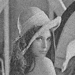
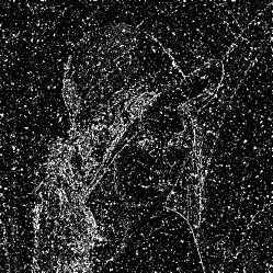
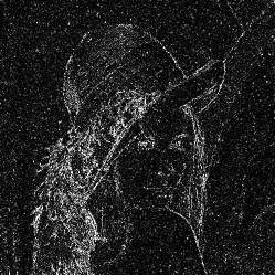
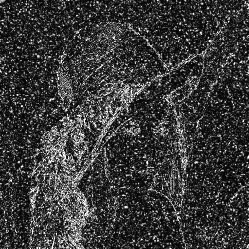
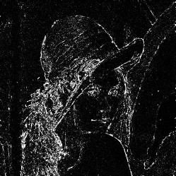
In (Garnett et al., 2005) it is suggested to take $d=1$ and $K=4$. For low and moderate levels of noise $(p<25\%)$, one iteration is sufficient and usually provides the best results; for high levels of noise $(p>25\%)$, applying two to five iterations provides better results. In our simulations, we found that a few spots of unremoved impulses often remain if we choose $d=1$ and $K=4$. This happens because impulses sometimes ”clump” together, and the $3\times 3$ detection window is too small to identify all the impulse noise points. Consequently, we select parameters $d=2$ and $K=12$ of detection windows for all levels of impulse noise. Figure 1 shows the comparison results between the restored images, with detection window $3\times 3$ and with detection window $5\times 5$, which have been added an impulse noise with $p=20\%$, $30\%,$ $40\%,$ and $50\%$ respectively. When $p=30\%$, $40\%$ and $50\%$, we can see clearly some impulse spots in the restored images with detection window $3\times 3$, while the visual quality of the restored images with detection window $5\times 5$ is very good, without impulse spots. In the case where $p=20\%$, impulse spots of the restored image with detection window $3\times 3$ are not obvious, and the PSNR value is a little better than that with detection window $5\times 5$, whereas Figure 2 shows that the first image has two clumpy impulse spots and the visual quality is not good enough. Consequently, we prefer detection window $5\times 5$ for all levels impulse noise.

Table 2: Performance of denoising algorithms when applied to test impulse noisy images.

Images	Baboon		Bridge		Lena		Pentagon
p%	$20\%$	$40\%$	$20\%$	$40\%$	$20\%$	$40\%$	$20\%$	$40\%$
Method	PSNR	PSNR	PSNR	PSNR	PSNR	PSNR	PSNR	PSNR
Our method
$M=13\times 13$	24.81db	22.12db	27.84db	24.91db	35.50db	32.19db	30.91db	28.34db
$m=25\times 25$
Sun and Neuvo (1994)	23.67db	20.85db	26.26db	22.66db	32.93db	27.90db	29.34db	26.26db
Abreu et al. (1996)	23.81db	21.49db	26.56db	23.80db	35.71db	29.85db	30.38db	27.27db
Wang and Zhang (1999)	23.43db	21.07db	26.33db	22.75db	35.09db	28.92db	29.18db	26.19db
Chen et al. (1999)	23.73db	21.38db	26.52db	22.89db	34.21db	28.30db	29.29db	26.29db
Chen and Wu (2001b)	24.02db	21.52db	27.27db	23.55db	35.44db	29.26db	30.34db	27.04db
Chen and Wu (2001a)	24.17db	21.58db	27.08db	23.23db	36.07db	28.79db	30.23db	26.84db
Crnojevic et al. (2004)	23.78db	21.56db	26.90db	23.83db	36.50db	31.41db	30.11db	27.33db
Wenbin (2005)	24.18db	21.41db	27.05db	23.88db	36.90db	30.25db	30.42db	26.93db
Garnett et al. (2005)	24.18db	21.60db	27.60db	24.01db	36.70db	31.12db	30.33db	27.14db
Chan et al. (2004)	23.97db	21.62db	27.31db	24.60db	36.57db	32.21db	30.03db	27.35db
Dong et al. (2007)	24.49db	21.92db	27.86db	24.79db	37.45db	32.76db	30.73db	27.73db
Yu et al. (2008)	24.86db	22.06db	28.06db	24.97db	36.18db	32.03db	-	-

Table 3: Comparison between the TriF (Garnett et al., 2005), and OWMF (Our method) in removing mixed noise.

Gaussian Noise	Image	Method	$p=0.2$	$p=0.3$	$p=0.4$	$p=0.5$
		Garnett et al. (2005)	31.48db	29.87db	28.57db	27.31db
	Lena	Our method	33.18db	32.05db	30.90db	29.52db
		Garnett et al. (2005)	25.82db	24.92db	23.79db	22.28db
	Bridge	Our method	26.42db	25.19db	24.08db	23.08db
sigma=10		Garnett et al. (2005)	28.61db	27.54db	26.22db	24.74db
	Boat	Our method	29.57db	28.22db	27.05db	25.92db
		Garnett et al. (2005)	24.82db	24.00db	23.08db	22.33db
	Barbara	Our method	28.47db	26.46db	24.83db	23.62db
		Garnett et al. (2005)	28.85db	28.02db	27.10db	25.68db
	Lena	Our method	30.87db	30.09db	29.19db	28.14db
		Garnett et al. (2005)	23.56db	23.01db	22.47db	21.72db
	Bridge	Our method	24.70db	23.97db	23.21db	22.45db
sigma=20		Garnett et al. (2005)	26.18db	25.46db	24.75db	23.79db
	Boat	Our method	27.79db	26.93db	25.97db	25.08db
		Garnett et al. (2005)	23.35db	22.95db	22.53db	21.84db
	Barbara	Our method	27.50db	25.95db	24.43db	23.33db
		Garnett et al. (2005)	27.26db	26.57db	25.58db	23.99db
	Lena	Our method	29.12db	28.49db	27.76db	26.75db
		Garnett et al. (2005)	22.88db	22.42db	21.87db	20.98db
	Bridge	Our method	23.56db	23.02db	22.49db	21.86db
sigma=30		Garnett et al. (2005)	25.11db	24.55db	23.80db	22.62db
	Boat	Our method	26.41db	25.79db	25.08db	24.26db
		Garnett et al. (2005)	22.82db	22.46db	21.94db	21.10db
	Barbara	Our method	25.98db	24.81db	23.72db	22.81db

$p=20\%$	$p=30\%$	$p=40\%$	$p=50\%$
PSNR=36.03db	PSNR=33.65db	PSNR=30.22db	PSNR=27.35db
PSNR=35.50db	PSNR=33.92db	PSNR=32.19db	PSNR=30.09db

Figure 1: The first row gives the levels of added impulse noise. The second and the third rows display images restored with detection window $3\times 3$, and their PSNR values. The forth and fifth rows show images restored with detection window $5\times 5$ and their PSNR values . The 1, 2, 3 and 4 columns give the restored images which have been contaminated by an impulse noise with $p=20\%$, $30\%,$ $40\%,$ and $50\%$ respectively.

Figure 2: The first and second $100\times 100$ images are parts of images restored with detection windows $3\times 3$ and $5\times 5$ respectively; the original image has been contaminated by an impulse noise with $p=20\%$.

We use the kernel $\kappa_{0}$ for computing the estimated brightness variation function $\widehat{\rho}_{J,\kappa,x_{0}},$ which corresponds to the Optimal Weights Mixed Filter as defined in Section 2.3. The parameters $m$ and $M$ have been fixed to $m=25\times 25$ and $M=13\times 13.$ In Figure 3, the images in the third row show that the noise is reduced in a natural manner and significant geometric features, fine textures, and original contrasts are visually well recovered with no undesirable artifacts. To better appreciate the accuracy of the restoration process, the images of square errors (the square of the difference between the original image and the recovered image) are shown in the fifth row of Figure 3, where the dark values correspond to a high-confidence estimate. As expected, pixels with a low level of confidence are located in the neighborhood of image discontinuities. For comparison, we show the images denoised by the trilateral filter TriF (see the images in the second row of Figure   3 ) and their square errors (see the images in the forth row of Figure   3). We can see clearly that the images of square errors of our methods are darker than that of Trif, so our method provides significant improvement over. The overall visual impression and the numerical results are improved using our algorithm.

For comparison, we consider follows three cases: pure Gaussian noise, pure impulse noise and the mixture of Gaussian and impulse noises. In the case of pure Gaussian white noise, we have done simulation on a commonly-used set of images (”Lena”, ”Barbara”, ”Boat” and ”House”) available at http://decsai.ugr.es/ javier/
denoise/test_images/ and the comparison with several filters is given in Table 1. The PSNR values show that our approach work as well as those sophisticated methods, like Hirakawa and Parks (2006), Kervrann and Boulanger (2008), Hammond and Simoncelli (2008) and Aharon et al. (2006), and is better than the filters proposed in Buades et al. (2005), Salmon and Le Pennec (2009), Katkovnik et al. (2004), Foi et al. (2004) and Roth and Black (2009). The proposed approach gives a quality of denoising which is competitive with that of the best recent method BM3D (see Dabov et al. (2007)). These methods can only deal wits pure Gaussian noise, while our method can not only cope with the Gaussian noise, but also remove the impulse noise and the mixture of Gaussian and pure impulse noises. For the pure impulse noise, our method is also competitive to the sophisticated method. In order to compare the others methods, we choose a commonly set of images (”Baboon”, ”Badge”, ”Lena” and ”Pentagon”) which is taken in (Dong et al., 2007). Table 2 lists the restoration results of well-know different algorithm. It is clear that our method provides significant improvement over Sun and Neuvo (1994), Abreu et al. (1996), Wang and Zhang (1999), Chen et al. (1999), Chen and Wu (2001b), Chen and Wu (2001a), Crnojevic et al. (2004), Wenbin (2005), etc. Our approach work as well as Dong et al. (2007) and Yu et al. (2008), when our approach produces the best PSNR values in the cases of ”Baboon” (40%) and ”Pentagon” (20% and 40%), while Yu et al. (2008) has the best results in the case of ”Baboon” (20%) and ”Bridge” (20% and 40%), and Dong et al. (2007)(ROLD-EPR) wins in the case of ”Lena” (20% and 40%). Finally, we show the comparison between the Garnett et al. (2005) and our method with the set of images (”Lena”, ”Bridge”, ”Boat” and ”Barbara”). From Table 3, it is clear that our method provides significant improvement over the algorithm Trif (Garnett et al., 2005).

$p=20$, $\sigma=0$	$p=20$, $\sigma=10$	$p=0$, $\sigma=20$

Figure 3: The first row is the images with different levels of mixture of impulse and Gaussian noise. The second and the third row display the images restored by TriF and OWMF respectively. The forth and the fifth row give square error image with TriF and OWMF respectively.

4 Conclusion

A new image denoising filter, which deal with the mixture of Gaussian and impulse noises model based on weights optimization and the modified Rank-Ordered Absolute Differences statistic, is proposed. The implementation of the filter is straightforward. Our work leads to the following conclusions.

1. The modified Rank-Ordered Absolute Differences statistic, used in the new filter, detects effectively the impulse noise in the case of mixture of Gaussian and impulse noises. This statistic is well adapted for use with the Weights Optimization Filter of (Jin et al., 2011).

2. The proposed filter is proven by simulations to be very efficient for removing both a mixture of impulse and Gaussian noises, and the pure impulse or pure Gaussian noise.

3. Our numerical results demonstrate that the new filter outperforms the known filters.

References

- Abreu et al. (1996) Abreu,E., Lightstone, M., Mitra, S.K., & Arakawa, K.(1996). A new efficient approach for the removal of impulse noise from highly corrupted images. IEEE Trans. Image Process., 5(6):1012–1025.
- Aharon et al. (2006) Aharon,M., Elad,M., & Bruckstein, A. (2006). -svd: An algorithm for designing overcomplete dictionaries for sparse representation. IEEE Trans. Signal Process., 54(11):4311–4322.
- Bouboulis et al. (2010) Bouboulis,P., Slavakis,K., & Theodoridis, S. (2010). Adaptive kernel-based image denoising employing semi-parametric regularization. IEEE Trans. Image Process., 19(6):1465–1479.
- Buades et al. (2005) Buades,A., Coll,B., & Morel,J.M. (2005). A non-local algorithm for image denoising. In in Proc. Int. Conf. Computer Vision and Pattern Recognition(CVPR), volume 2, pages 60–65. IEEE.
- Cai et al. (2008) Cai,J.F., Chan,R.H., & Nikolova,M. (2008). Two-phase approach for deblurring images corrupted by impulse plus Gaussian noise. Inverse Probl. Imag., 2(2):187–204.
- Chan et al. (2004) Chan,R.H., Hu,C., & Nikolova,M. (2004). An iterative procedure for removing random-valued impulse noise. IEEE Signal Proc. Let., 11(12):921–924.
- Chen and Wu (2001a) Chen,T., & Wu, H.R. (2001a). Adaptive impulse detection using center-weighted median filters. IEEE Signal Process. Lett., 8(1):1–3.
- Chen and Wu (2001b) Chen,T., & Wu,H.R.(2001b). Space variant median filters for the restoration of impulse noise corrupted images. IEEE T Circuits-II, 48(8):784–789.
- Chen et al. (1999) Chen, T., Ma,K.K., & Chen, L.H.(1999). Tri-state median filter for image denoising. IEEE Trans. Image Process., 8(12):1834–1838.
- Crnojevic et al. (2004) Crnojevic,V., Senk,V., & Trpovski,Z.(2004). Advanced impulse detection based on pixel-wise mad. IEEE Signal Process. Lett., 11(7):589–592.
- Dabov et al. (2007) Dabov,K., Foi,A., Katkovnik,V., & Egiazarian,K.(2007). Image denoising by sparse 3-D transform-domain collaborative filtering. IEEE Trans. Image Process., 16(8):2080–2095. ISSN 1057-7149.
- Dong et al. (2007) Dong,Y., Chan,R.H., & Xu,S.(2007). A detection statistic for random-valued impulse noise. IEEE Trans. Image Process., 16(4):1112–1120.
- Foi et al. (2004) Foi,A., Katkovnik,V., Egiazarian,K., & Astola,J.(2004). A novel anisotropic local polynomial estimator based on directional multiscale optimizations. In Proc. 6th IMA int. conf. math. in signal process., pages 79–82. Citeseer.
- Garnett et al. (2005) Garnett,R., Huegerich,T., Chui,C., & He,W.(2005). A universal noise removal algorithm with an impulse detector. IEEE Trans. Image Process., 14(11):1747–1754. ISSN 1057-7149.
- Hammond and Simoncelli (2008) Hammond,D.K., & Simoncelli, E.P.(2008). Image modeling and denoising with orientation-adapted gaussian scale mixtures. IEEE Trans. Image Process., 17(11):2089–2101.
- Hirakawa and Parks (2006) Hirakawa,K., & Parks,T.W.(2006) Image denoising using total least squares. IEEE Trans. Image Process., 15(9):2730–2742.
- Hwang and Haddad (1995) Hwang,H., & Haddad,R.A.(1995). Adaptive median filters: new algorithms and results. IEEE Trans. Image Process., 4(4):499–502.
- Jin et al. (2011) Jin,Q., Grama,I., & Liu,Q.(2011). Removing gaussian noise by optimization of weights in non-local means. Arxiv preprint arXiv:1109.5640.
- Katkovnik et al. (2004) Katkovnik,V., Foi,A., Egiazarian,K., & Astola,J.(2004). Directional varying scale approximations for anisotropic signal processing. In Proc. XII European Signal Proc. Conf., EUSIPCO 2004, Vienna, pages 101–104.
- Katkovnik et al. (2010) Katkovnik,V., Foi,A., Egiazarian, K., & Astola,J.(2010). From local kernel to nonlocal multiple-model image denoising. Int. J. Comput. Vis., 86(1):1–32. ISSN 0920-5691.
- Kervrann and Boulanger (2006) Kervrann,C., & Boulanger,J.(2006). Optimal spatial adaptation for patch-based image denoising. IEEE Trans. Image Process., 15(10):2866–2878. ISSN 1057-7149.
- Kervrann and Boulanger (2008) Kervrann,C., & Boulanger,J.(2008). Local adaptivity to variable smoothness for exemplar-based image regularization and representation. Int. J. Comput. Vis., 79(1):45–69. ISSN 0920-5691.
- Li et al. (2010) Li,B., Liu,Q.S., Xu,J.W., & Luo,X.J.(2010). A new method for removing mixed noises. Sci. China Ser. F (Information sciences), 54:1–9. ISSN 1674-733X.
- Lou et al. (2010) Lou,Y., Zhang, X., Osher,S., & Bertozzi,A.(2010). Image recovery via nonlocal operators. J. Sci. Comput., 42(2):185–197. ISSN 0885-7474.
- Luisier et al. (2011) Luisier,F., Blu,T., & Unser,M.(2011). Image denoising in mixed poisson-gaussian noise. IEEE Trans. Image Process., (99):1–1.
- Nikolova (2004) Nikolova,M.(2004). A variational approach to remove outliers and impulse noise. J. Math. Imaging. Vis., 20(1):99–120.
- Polzehl and Spokoiny (2000) Polzehl,J., & Spokoiny,V.G.(2000). Adaptive weights smoothing with applications to image restoration. J. Roy. Stat. Soc. B, 62(2):335–354. ISSN 1369-7412.
- Roth and Black (2009) Roth,S., & Black,M.J.(2009). Fields of experts. Int. J. Comput. Vision, 82(2):205–229.
- Salmon and Le Pennec (2009) Salmon,J., & Le Pennec,E.(2009). Nl-means and aggregation procedures. In IEEE Int. Conf. Image Process. (ICIP), pages 2977–2980. IEEE.
- Sun and Neuvo (1994) Sun,T., & Neuvo, Y.(1994). Detail-preserving median based filters in image processing. Pattern Recognition Letters, 15(4):341–347.
- Wang and Zhang (1999) Wang,Z., & Zhang,D.(1999). Progressive switching median filter for the removal of impulse noise from highly corrupted images. IEEE Trans. Circuits Syst. II, Analog Digit. Signal Process., 46(1):78–80.
- Wenbin (2005) Luo W.(2005). A new efficient impulse detection algorithm for the removal of impulse noise. IEICE Trans. Fundam., 88:2579–2586.
- Xiao et al. (2011) Xiao,Y., Zeng,T., Yu,J., & Ng,M.K.(2011). Restoration of images corrupted by mixed gaussian-impulse noise via (l1)-(l0) minimization. Patteen Recogn..
- Yu et al. (2008) Yu,H., Zhao,L., & Wang,H. (2008). An efficient procedure for removing random-valued impulse noise in images. IEEE Signal Process. Lett., 15:922–925.