A family of sand automata

Abstract

We study some dynamical properties of a family of two-dimensional cellular automata: those that arise from an underlying one dimensional sand automaton whose local rule is obtained using a latin square. We identify a simple sand automaton $\Gamma$ whose local rule is algebraic, and classify this automaton as having equicontinuity points, but not being equicontinuous. We also show it is not surjective. We generalise some of these results to a wider class of sand automata.

1 Introduction

In [CFM07], the authors introduce the family of sand automata: these are dynamical systems $\Phi:{\mathcal{A}}^{{\mathbb{Z}}^{d}}\rightarrow{\mathcal{A}}^{{\mathbb{Z}}^{d}}$, where $\mathcal{A}$ is an countably infinite alphabet, that satisfy certain constraints (see Section 2 for all definitions). In turn, with the appropriate topology $\mathcal{T}$ put on ${\mathcal{A}}^{{\mathbb{Z}}^{d}}$, $({\mathcal{A}}^{{\mathbb{Z}}^{d}},\Phi)$ is topologically conjugate to a cellular automaton $\Phi_{{{1}\choose{0}}}:S_{{{1}\choose{0}}}\rightarrow S_{{{1}\choose{0}}}$ where $S_{{{1}\choose{0}}}\subset\{0,1\}^{{\mathbb{Z}}^{d+1}}$ is a subshift of finite type. In [DGM09] the authors ask if any of the cellular automata arising from sand automata are chaotic. This is a particular instance of the more general project of finding chaotic higher dimensional cellular automata. In this article we study a family of sand automata and their dynamical properties.

In Section 2.5, we define linear sand automata: these are automata whose local rules are built using a group endomorphism $\phi:{\mathcal{A}}^{2r+1}\rightarrow{\mathcal{A}}$, where the finite alphabet $\mathcal{A}$ is viewed as a cyclic group. We say that local rules are ‘built’, because, unlike cellular automata, the initial configuration has to be relativised before the local rule is applied, and the output of the local rule is added to the initial configuration. In general we work exclusively with one dimensional sand automata (ie those whose corresponding cellular automata act on two dimensional configuration space), whose local rules have radius 1. We frequently work with one fixed sand automaton, $\Gamma:{\mathcal{A}}^{\mathbb{Z}}\rightarrow{\mathcal{A}}^{\mathbb{Z}}$, whose local rule is built using the rule $\gamma:{\mathbb{Z}}_{5}^{3}\rightarrow{\mathbb{Z}}_{5}$ defined by $\gamma({x_{-1}\,x_{0}\,x_{1}})=x_{-1}+x_{1}$, which is the local rule for the famous XOR cellular automaton (albeit on a different alphabet), and whose dynamical properties have been studied extensively, for example in [MM98], [CFMM97] and [IÔN83].

Although we are interested in the dynamical properties of the cellular automaton $\Phi_{{{1}\choose{0}}}$, in practice we often work with $\Phi$, since all of the dynamical properties that we discuss are topological invariants. In Section 3, we show that $\Gamma$ is not surjective - recall that a cellular automaton which is not surjective cannot be transitive. In Section 3.1, we identify a proper $\Gamma$-invariant subspace, ${\mathcal{G}}$, and show that for points ${\bf x}$ in ${\mathcal{G}}$, computation of $\Gamma^{n}(x)$ is simple, for all $n$. We identify other sand automata for which ${\mathcal{G}}$ acts similarly - this accounts for about 17% of all radius one sand automata, all of which cannot be transitive.

In Section 4 we show that $\Gamma$ is not equicontinuous, by showing the existence of (many) vertical inducing points. In fact all radius one sand automata whose local rule tables have, for some non-zero $m$, the value $m$ appear in each column (or each row), have vertical inducing points, and so are not equicontinuous. This means that at least $99\%$ of all sand automata are not equicontinuous. Despite not being equicontinuous, we show that $\Gamma$ has equicontinuity points by finding a blocking word for $\Gamma$. This completes the classification of $\Gamma$ according to the classification scheme in [DGM09].

In Section 4.2, we generalise the definition of a vertical inducing point to that of a local rule constant point. Both vertical inducing and local rule constant points have easily computable $\Phi^{n}$ iterates. We identify a $\Gamma$-invariant subspace $\mathcal{G}^{*}$, in which all points are local rule constant. We define a subspace $\mathcal{G}^{\prime}$ containing $\mathcal{G}^{*}$, and conjecture that $\mathcal{G}^{\prime}$ is an attractor for $\Gamma$, in that $\lim_{n\rightarrow\infty}d(\Gamma^{n}{\bf x},\mathcal{G}^{\prime})=0$ whenever ${\bf x}\in{\mathcal{A}}^{\mathbb{Z}}$.

2 Preliminaries

2.1 Notation

If $\mathcal{A}$ is a countable alphabet, let $\mathcal{A}^{+}$ the set of finite concatenations of letters from $\mathcal{A}$; elements of $\mathcal{A}^{+}$ are called words. If $d$ is a natural number, we let $X=\mathcal{A}^{\mathbb{Z}^{d}}:=\{\textbf{x}=\{(x_{{\bf n}})_{{\bf n}\in\mathbb{Z}^{d}}:x_{{\bf n}}\in\mathcal{A}\mbox{ for each }{\bf n}\in\mathbb{Z}^{d}\}$; we call $X$ the $d$-dimensional configuration space on the alphabet $\mathcal{A}$, and elements of $X$ are called configurations. If ${\bf x}\,\in\mathcal{A}^{\mathbb{Z}}$, we sometimes write ${\bf x}=\ldots x_{-1}.x_{0}x_{1}\ldots$. If $\textbf{x}\in\mathcal{A}^{\mathbb{Z}},\,m,n\in\mathbb{Z},\,m\leq n$ let $\textbf{x}_{[m,n]}:=x_{m}x_{m+1}\ldots x_{n}$. We will be working in dimensions 1 and 2, and in dimension 2 only when $\mathcal{A}$ is finite.

We let $\mathcal{A}_{r}:=\{-r,\ldots,r\}$, and, if $\mathcal{A}$ is given, let $\widetilde{\mathcal{A}}=\mathcal{A}\cup\{-\infty,\infty\}$. Loosely speaking if $d=2$ then x represents a 3-dimensional sandpile where $x_{{\bf n}}$ represents the number of sand grains at “location” ${\bf n}$. If $x_{{\bf n}}=\infty$ there is a source at location ${\bf n}$ and if $x_{{\bf n}}=-\infty$ there is a sink at location ${\bf n}$.

Let $L\subset{\mathcal{A}}^{\mathbb{Z}^{d}}$ be a finite set. If ${\bf c}=\{c_{\bf l}:c_{\bf l}\in\mathcal{A},\mbox{ for }{\bf l}\in\mathbb{Z}_{d}\cap L\}$, define the cylinder set $[{\bf c}]=\{x:x_{\bf l}=c_{\bf l},\mbox{ for }{\bf l}\in L\}$. If $\mathcal{A}$ is finite the Cantor topology - generated by the cylinder sets, as $L$ and ${\bf c}$ vary - makes ${\mathcal{A}}^{\mathbb{Z}^{d}}$ compact. If $\mathcal{A}=\widetilde{\mathbb{Z}}$ this is no longer the case. Because of this it is convenient to embed $\widetilde{\mathbb{Z}}^{\mathbb{Z}}$ in $\{0,1\}^{\mathbb{Z}^{2}}$, and equip it with the subspace topology $\mathcal{T}$ that it inherits from $\{0,1\}^{\mathbb{Z}^{2}}$: this is what is done in [DGM09]. Define the map $e:{\widetilde{\mathbb{Z}}}^{\mathbb{Z}}\rightarrow\{0,1\}^{\mathbb{Z}^{2}}$ by

$$(e(\textbf{x}))_{i,j}=\left\{\begin{array}[]{rl}1&\textit{if }j\leq x_{i}\\ 0&\textit{if }j>x_{i}\\ \end{array}\right.\,.$$

In other words, the amount of sand $x_{i}$ at location $i$ in ${\bf x}$ is recorded in the $i$th column of $e({\bf x})$, where there are ones for all column entries that are indexed by at most $x_{i}$, and zeros above entry $x_{i}$. If $x_{i}=\infty$, the $i$-th column of $e({\bf x})$ is constantly 1, and similarly if $x_{i}=-\infty$ the $i$-th column of $e({\bf x})$ is constantly 0.

The transformation $e:X\rightarrow e(X)$ is bijective and its image $e(X)$ is a subshift of finite type, where the unique forbidden word is $\begin{array}[]{|c|c|}\hline\cr 1\\ \hline\cr 0\\ \hline\cr\end{array}$. If $\{0,1\}^{\mathbb{Z}^{2}}$ is equipped with the Cantor topology then since $e(X)$ is closed in $\{0,1\}^{\mathbb{Z}^{2}}$, it is also compact. Let $\mathcal{T}$ be the topology on $X={\widetilde{\mathbb{Z}}}^{\mathbb{Z}}$ inherited from the subspace topology on $e(X)\subset\{0,1\}^{{\mathbb{Z}}^{2}}$.

2.2 Dynamical systems

We recall some basic definitions. If $X$ is a topological space and $F:X\rightarrow X$ be continuous, then $(X,F)$ is a topological dynamical system. $(X,F)$ is transitive if for all nonempty open sets $U,V\subseteq X,\exists n\geq 0$ such that $F^{-n}(U)\cap V\neq\emptyset$. $(X,F)$ is equicontinuous at $x\in X$ if $\forall\epsilon>0,\exists\delta>0,\forall y\in B_{\delta}(x),\forall n>0,d(F^{n}(x),F^{n}(y))<\epsilon$; and $(X,F)$ is equicontinuous if $F$ is equicontinuous at all points in $X$. $(X,F)$ is sensitive to initial conditions if $\exists\epsilon>0,\forall x\in X,\forall\delta>0,\exists y\in B_{\delta}(x),\exists n>0,d(F^{n}(x),F^{n}(y))>\epsilon$. Finally $(X,F)$ is positively expansive if $\exists\epsilon>0,\forall x\neq y,\exists n\geq 0,d(F^{n}(x),F^{n}(y))\geq\epsilon$. A point $x\in X$ is periodic if $F^{n}(x)=x$ for some $n$; if $n=1$ then $x$ is fixed. We call the smallest such $n$ the period of x. The point $x\in X$ is eventually periodic if $\exists p,n\in\mathbb{N}$ such that $F^{p+n}(x)=F^{p}(x)$; we call $p$ the preperiod. A dynamical system is ultimately periodic if $\forall x\in X$, x is eventually periodic.

A dynamical system is chaotic if is sensitive, transitive and has a dense set of periodic points. In [BBC⁺92] it is shown that if $(X,F)$ is transitive and has a dense set of periodic points then $(X,F)$ is sensitive. In [CM96], the authors show that if $(X,F)$ is a cellular automaton (see below for definitions) then transitivity alone implies sensitivity.

2.3 Cellular and sand automata

Let $X={\mathcal{A}}^{\mathbb{Z}}$ where $\mathcal{A}$ is a finite alphabet. A cellular automaton $F:X\rightarrow X$ is a map defined by a local rule $f:{\mathcal{A}}^{2r+1}\rightarrow\mathcal{A}$, so that for each $n\in\mathbb{Z}$, $(F({\bf x}))_{n}=f(x_{n-r},\ldots x_{n+r})$. The simplest example of a cellular automaton is the shift map $\sigma:X\rightarrow X$, where $(\sigma({\bf x}))_{n}=x_{n+1}$. If $X={\mathcal{A}}^{\mathbb{Z}^{d}}$, a cellular automaton can be defined similarly: if $L_{r}:=\{{\bf l}:{\bf l}=(l_{1},l_{2}),\,\,|l_{i}|\leq r\}$ is the 2-dimensional box of radius $r$, and $f:{\mathcal{A}}^{L_{r}}\rightarrow{\mathcal{A}}$ is a map, then a cellular automaton $F:{\mathcal{A}}^{\mathbb{Z}^{2}}\rightarrow{\mathcal{A}}^{\mathbb{Z}^{2}}$ is defined as $(F({\bf x}))_{\bf n}=f(\{x_{\bf n+i}:{\bf i}\in L_{r}\}).$ There are two shift maps on two-dimensional lattice spaces $X={\mathcal{A}}^{{\mathbb{Z}}^{d}}$: let $(\sigma_{H}({\bf x}))_{{\bf n}}=x_{{\bf n}+(1,0)}$, $(\sigma_{V}({\bf x}))_{{\bf n}}=x_{{\bf n}+(0,1)}$ be the horizontal and vertical shifts respectively. In [Hed69], Hedlund showed that $F$ is a cellular automaton if and only if $F$ is a continuous, shift commuting map.

Let $X=\widetilde{\mathbb{Z}}^{\mathbb{Z}}$. Like cellular automata, sand automata are defined in [CFM07] as functions $\Phi:X\rightarrow X$ which have a local rule $\phi$, except that the output of the local rule is added to the original entry. First, in [CFM07] the authors define a sequence of “measuring instruments” of precision $r$. If $n\in\mathbb{N}$ and $m\in\mathbb{Z}$ then the measuring tool of precision $r$ at reference height $m$ is the function $\beta_{r}^{m}:\widetilde{\mathbb{Z}}\rightarrow\widetilde{\mathcal{A}_{r}}$ where

$$\beta_{r}^{m}(n)=\left\{\begin{array}[]{ll}+\infty&\mbox{ if }n>m+r,\\ -\infty&\mbox{ if }n<m-r,\\ n-m&\mbox{ otherwise.}\\ \end{array}\right.$$ (2.1)

Let $\phi:\widetilde{\mathcal{A}_{r}}^{2r}\rightarrow\mathcal{A}_{r+1}$ be given. Define

$$\Phi(\textbf{x})_{i}=\left\{\begin{array}[]{ll}x_{i}+\phi(\beta_{r}^{x_{i}}(x_{i-r}),\ldots\beta_{r}^{x_{i}}(x_{i-1}),\beta_{r}^{x_{i}}(x_{i+1}),\ldots\beta_{r}^{x_{i}}(x_{i+r}))&\mbox{if }x_{i}\in\mathbb{Z}\\ x_{i}&\mbox{ if }x_{i}=\pm\infty\\ \end{array}\right.$$

Thus $\Phi(\textbf{x})_{i}$ differs from $x_{i}$ by at most $r+1$, and is a function of the cylinder $x_{[i-r,i+r]}$. Note that $\phi$ is applied not to $x_{[i-r,i+r]}$ but to a relativised version of this word.

As a book-keeping device we define a projection $\Pi:X\rightarrow\{\widetilde{\mathcal{A}}^{2r}_{r}\}^{\mathbb{Z}}$ by $\Pi(\textbf{x})_{i}=\beta_{r}^{x_{i}}(x_{i-r}),\ldots\beta_{r}^{x_{i}}(x_{i-1}),\beta_{r}^{x_{i}}(x_{i+1}),\ldots\beta_{r}^{x_{i}}(x_{i+r})$. Clearly $\Pi$ is not injective. We refer to $\Pi(\textbf{x})_{i}$ as a gradient tuple, and later in this article we use $L_{1},\ldots L_{r}$ to describe the gradients to the left of the reference position and $R_{1},\ldots R_{r}$ to describe the gradients to the right of the reference position.

Example 2.1.

This is Example 12 in [CFM07], which emulates the behaviour of the original model defined in [BTW88]. Define a 1 dimensional sand automaton $F$ whose local rule $\phi:\widetilde{\mathcal{A}_{1}}^{2}\rightarrow\mathcal{A}_{1}$ is given by:

$$\phi(a,b)=\left\{\begin{array}[]{ll}1&\mbox{ if }a=\infty,\,b\neq-\infty\\ -1&\mbox{ if }a\neq\infty,\,b=-\infty\\ 0&\mbox{ otherwise }\\ \end{array}\right.$$

$F$ has the property that a grain of sand falls to the right (and only the right) if the right neighbour is at least 2 smaller. If the number of sand grains in the initial configuration ${\bf x}$ is finite, then $F^{n}(x)$ is eventually fixed.

Define the vertical map $\rho:X\rightarrow X$ where

$$\rho(\textbf{x})_{i}=\left\{\begin{array}[]{ll}x_{i}+1&\mbox{ if }|x_{i}|<\infty,\\ x_{i}&\mbox{ if }|x_{i}|=\infty,\\ \end{array}\right.$$

and say that $\Phi$ is vertical commuting if $\Phi(\rho(x))=\rho(\Phi(x))$. Also, say that $\Phi$ is infiniteness conserving if $\Phi(\textbf{x})_{i}=\pm\infty\Leftrightarrow x_{i}=\pm\infty$. Note that all sand automata are shift commuting, vertical commuting, and infiniteness conserving; in fact this characterises them, as shown in Theorem 17 of [CFM07]:

Theorem 2.2.

$\Phi:X\rightarrow X$ is a sand automaton if and only if $\Phi$ is continuous, shift commuting, vertical commuting and infiniteness conserving.

The number $r$ in the definitions of cellular and sand automata is called the radius. In this article we only consider sand automata of radius 1.

2.4 Modelling sand automata as cellular automata

Using the injection $e:{\widetilde{\mathbb{Z}}}^{\mathbb{Z}}\rightarrow\{0,1\}^{{\mathbb{Z}}^{2}}$, we can transform a sand automaton into a 2-dimensional cellular automaton as done in [DGM09]. Letting $S_{{{1}\choose{0}}}$ denote $e(X)$, define $\Phi_{{{1}\choose{0}}}=e\circ\Phi\circ e^{-1}:S_{{{1}\choose{0}}}\rightarrow S_{{{1}\choose{0}}}$. With this notation, we have the following lemma, whose proof is straightforward:

Lemma 2.3.

$\Phi_{{{1}\choose{0}}}$ commutes with both the vertical and horizontal shifts, and if $X$ is endowed with the topology $\mathcal{T}$, then $(X,F)\cong(S_{{{1}\choose{0}}},\Phi_{{{1}\choose{0}}})$.

2.5 Linear sand automata

If $|\mathcal{A}|=2k+1$, then $\mathcal{A}$ can be viewed as the additive group $\mathbb{Z}_{2k+1}=\{-k,\ldots,0,\ldots,k\}$. Recall that $F:{\mathbb{Z}}_{2k+1}^{\mathbb{Z}}\rightarrow{\mathbb{Z}}_{2k+1}^{\mathbb{Z}}$ is a linear cellular automaton if its local rule $f:\mathbb{Z}_{2k+1}^{2r+1}\rightarrow\mathbb{Z}_{2k+1}$ is a group homomorphism. Thus $f(\textbf{x}_{[i-r,i+r]})=a_{0}x_{i-r}+a_{1}x_{i-r+1}+\ldots+a_{2r+1}x_{i+r}$ where $a_{i}$ and $x_{i}$ $\in\mathbb{Z}_{2k+1}$ for $0\leq i\leq 2r+1$. The topological properties of $F$ depend on the coefficients $a_{i}$: for example if the $a_{i}^{\prime}s$ are relatively prime, then $F$ is topologically transitive, so that many linear cellular automata are chaotic.

Next we describe how to define a sand automaton using a linear cellular automaton. Recall we only consider sand automata of radius 1. In this case we can display the local rule in terms of a local rule table. A local rule table has a row for each possible left gradient $L$ and a column for each possible right gradient $R$. Entry $(L,R)$ of the table is $\phi(L,R)$. For example, Figure 1 is the local rule table for the sand automaton $\Omega$ defined in Section 2.3. The local rule table is applied after each gradient pair is calculated. For example, if $\textbf{x}=\ldots,4,\cdot 2,1,\ldots$ then $(\Pi(x))_{0}={{\infty}\choose{-1}}$, so $L=\infty$ and $R=-1$, so that $(\Omega({\bf x}))_{0}=x_{0}+1=3$.

$L\backslash R$	$-\infty$	-1	0	1	$\infty$
$-\infty$	-1	0	0	0	0
-1	-1	0	0	0	0
0	-1	0	0	0	0
1	-1	0	0	0	0
$\infty$	0	1	1	1	1

Figure 1: The local rule table for the sand automaton $\Omega$.

We now define linear sand automata of radius $r$. Recall that to define $(F({\bf x}))_{0}$ first we relativise, sending $(x_{-1},x_{0},x_{1})$ to $(\beta^{x_{0}}_{1}(x_{-1}),\beta^{x_{0}}_{1}(x_{1}))\in\widetilde{\mathcal{A}}_{1}^{2}$. Let $f:\widetilde{\mathcal{A}}_{1}\rightarrow\mathbb{Z}_{5}$ be the bijection defined by

$$(f(x))_{i}=\left\{\begin{array}[]{ll}2&\mbox{ if }x_{i}=\infty\\ 1&\mbox{ if }x_{i}=1\\ 0&\mbox{ if }x_{i}=0\\ -1&\mbox{ if }x_{i}=-1\\ -2&\mbox{ if }x_{i}=-\infty\end{array}\right.$$

Given a group homomorphism $\phi^{*}:\mathbb{Z}_{5}^{2}\rightarrow\mathbb{Z}_{5}$, we say that a sand automaton $\Phi$ is a linear sand automaton if the local rule $\phi=\phi^{*}\circ f\circ\Pi$.

Example 2.4.

Let $\gamma_{*}:\mathbb{Z}_{5}^{2}\rightarrow\mathbb{Z}_{5}$ be defined by $\gamma_{*}(x,y)=x\oplus y$.

Let $\Gamma$ be the linear sand automaton with local rule $\gamma=\gamma_{*}\circ f\circ\Pi$. Then $\Gamma$ is a radius 1 linear sand automaton. The local rule table in Figure 2 corresponds to the group homomorphism $\gamma_{*}$. Note that here the rows and columns are indexed by ${\mathbb{Z}}_{5}$.

$L\backslash R$	-2	-1	0	1	2
-2	1	2	-2	-1	0
-1	2	-2	-1	0	1
0	-2	-1	0	1	2
1	-1	0	1	2	-2
2	0	1	2	-2	-1

Figure 2: The local rule table for $\Gamma$

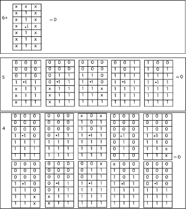
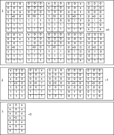
Figure 6: The local rule table for $\Gamma_{{{1}\choose{0}}}$. The number on the left of each rectangle represents the number of ones in the reference column. An ‘x’ represents a cell that can have any value. The $\cdot$ represents the central cell. Only configurations where the central cell changes are listed.

In this article we will often be working with $\Gamma$, even though we are interested primarily in $\Gamma_{{{1}\choose{0}}}$ (see Lemma 2.3). For, $\Gamma_{{{1}\choose{0}}}$ has radius $r=7$ (in fact the local neighbourhood can be a 7x3 rectangle) grid, so it is often more practical to work with the radius one $\Gamma$. Figure 6 contains the local rule table for $\Gamma_{{{1}\choose{0}}}$.

3 Non-surjectivity of $\Gamma$

A non-surjective sand automaton $F$ has Garden of Eden states: these are configurations that have no $F$-pre-image. A non-surjective cellular automaton cannot be chaotic, since it cannot be transitive. The surjectivity of sand automata is shown to be undecidable in [CFM07]. In this section we show that the sand automaton $\Gamma$ is not surjective, and generalise this result to some other one dimensional sand automata.

Recall that a sand automaton $\Phi:X\rightarrow X$ is surjective on a set $Y\subset X$ if for each ${\bf y}\in Y,$ $\Phi({\bf y^{\prime}})=\textbf{y}$ for some ${\bf y^{\prime}}\in Y$. A configuration is finite if all configuration entries are finite, and only finitely many entries are non-zero; let $\mathcal{F}$ denote all such points. Similarly, let $\mathcal{P}$ denote the set of all $\sigma$-periodic configurations, all of whose entries are finite. In [CFM07] (Proposition 3.14), the following was shown:

Lemma 3.1.

[[CFM07]] Let $\Phi:X\rightarrow X$ be a one-dimensional sand automaton. Then

1. $\Phi$ is surjective on $\mathcal{P}$ if and only if $\Phi$ is surjective, and

2. If $\Phi$ is surjective on $\mathcal{F}$, then $\Phi$ is surjective.

We show that $\Gamma$ is not surjective by first showing that there is a word which has no predecessor word under $\Gamma$. In the following proof the notation $[n]_{5}$ denotes the projection of $n\in\mathbb{Z}$ to $\mathbb{Z}_{5}$.

Lemma 3.2.

Let $\textbf{w}=(100,\,3,\,2,\,100)$. Then there is no word y such that $\Gamma(\textbf{y})=\textbf{w}$.

Proof.

Suppose that $\textbf{y}=y_{0}\,y_{1}\,y_{2}\,y_{3}\,y_{4}\,y_{5}$ is a word of length 6 such that $\Gamma(\textbf{y})=\textbf{w}$. Then

$$98\leq y_{1}\leq 102,\,\,\,1\leq y_{2}\leq 5,\,\,\,0\leq y_{3}\leq 4,\mbox{ and }98\leq y_{4}\leq 102\,.\,\,\,$$

This implies that $\beta_{1}^{y_{2}}(y_{1})=\beta_{1}^{y_{3}}(y_{4})=\infty$, ie $f(\beta_{1}^{y_{2}}(y_{1}))=f(\beta_{1}^{y_{3}}(y_{4}))=f(\infty)=2$. Next under the action of $\Gamma$ we have:

$$y_{2}+f(\beta_{1}^{y_{2}}(y_{1}))+f(\beta_{1}^{y_{2}}(y_{3}))=y_{2}+2+f(\beta_{1}^{y_{2}}(y_{3}))=3$$ (3.2)

$$y_{3}+f(\beta_{1}^{y_{3}}(y_{4}))+f(\beta_{1}^{y_{3}}(y_{2}))=y_{3}+2+f(\beta_{1}^{y_{3}}(y_{2}))=2$$ (3.3)

Projecting (3.2) and (3.3) into $\mathbb{Z}_{5}$, we have

$$[y_{2}]_{5}\oplus 2\oplus[y_{3}-y_{2}]_{5}=-2$$ (3.4)

$$[y_{3}]_{5}\oplus 2\oplus[y_{2}-y_{3}]_{5}=2$$ (3.5)

Adding (3.4) and (3.5) we get

$$[y_{2}]_{5}\oplus[y_{3}]_{5}=1$$ (3.6)

Thus the only possibilities for $[y_{2}]_{5}$ and $[y_{3}]_{5}$ are given by:

$[y_{2}]_{5}$ / $[y_{3}]_{5}$	-2	-1	0	1	2
-2	x
-1					x
0				x
1			x
2		x

This implies that the only possibilities for $y_{2},y_{3}$ are:

$y_{2}$ / $y_{3}$	3	4	0	1	2
3	x
4					x
5				x
1			x
2		x

Each of these cases implies a contradiction to Equation (3.6).

∎

Proposition 3.3.

$\Gamma$ is not $\mathcal{P}$-surjective, so that $\Gamma$ is not surjective.

Proof.

Let ${\bf x}$ be the periodic configuration ${\bf x}=\overline{100,\,3,\,2,\,100,}\cdot\overline{100,\,3,\,2,\,100}$. Lemma 3.2 implies that there does not exist ${\bf y}$ such that $\Gamma({\bf y})={\bf x}$. Lemma 3.1 implies that $\Gamma$ is not surjective. ∎

3.1 Surjective subsets

While $\Gamma$ is not surjective, in this section we identify a proper, closed, $\Gamma$-invariant subspace, $\mathcal{G}$. We then identify sand automata $\Phi$ for which $\mathcal{G}$ is also $\Phi$-invariant. Let

$${\mathcal{G}}:=\{\textbf{x}:|x_{i}-x_{i-1}|\geq 2,\,\forall i\}\,.$$

We shall show that each member of $\mathcal{G}$ has a $\Gamma$-predecessor (though not necessarily in $\mathcal{G}$). We will explain in geometric terms how $\Gamma$ acts on $\mathcal{G}$, identify subsets of $\mathcal{G}$ that are a possible attractor for $\Gamma$, and generalize these properties to other sand automata.

It is clear that $f\circ\Pi({\mathcal{G}})\subset\{{{2}\choose{2}},{{-2}\choose{2}},{{2}\choose{-2}},{{-2}\choose{-2}}\}^{\mathbb{Z}}$, and that $f\circ\Pi({\mathcal{G}})$ is the subshift of finite type whose transition graph $G$ is shown in Figure 3. Re-label ${{2}\choose{2}}=-1,{{-2}\choose{2}}=0^{-},{{2}\choose{-2}}=0^{+},{{-2}\choose{-2}}=1$, and let $Y_{G}$ denote the image of $f\circ\Pi(\mathcal{G})$ under this labelling. Let $\{-1,0,1\}^{\mathbb{Z}}$ be the full shift on three letters and let $p:\{0^{-},0^{+},1,-1\}\rightarrow\{-1,0,1\}$ by defined by $p(0^{-})=p(0^{+})=0,$ $p(1)=1$, $p(-1)=-1$; then p is a radius 0 local rule for the cellular automaton $P:Y_{G}\rightarrow\{-1,0,1\}^{\mathbb{Z}}$. With this notation, the following lemma is straightforward.

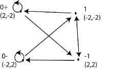
Figure 3: This graph $G$ defines a subshift on its bi-infinite paths.

Lemma 3.4.

If ${\bf g}\in{\mathcal{G}}$ then $\exists{\bf y}\in Y_{G}$ such that $\Gamma({\bf g})={\bf g}+P({\bf y})$.

$L\backslash R$	-2	2
-2	1	0
2	0	-1

Table 1: The local rule table for $\Gamma$ restricted to $\mathcal{G}$

On $\mathcal{G}$ the local rule table for $\Gamma$ can be compressed to Table 1. Call 3-tuples such that $f\circ\Pi(a,b,c)={{-2}\choose{-2}}$ peaks (centred at $b$) and similarly $f\circ\Pi(a,b,c)={{2}\choose{2}}$ valleys (centred at $b$). Also label 3-tuples such that $f\circ\Pi(a,b,c)={{-2}\choose{2}}$ up-slopes (centred at b) and $f\circ\Pi(a,b,c)={{2}\choose{-2}}$ down-slopes (centred at b). With this labelling of gradient tuples as geographical features, the action of $\Gamma^{n}$ is easily described, once we have knowledge of how $\Gamma$ acts.

Proposition 3.5.

If ${\bf g}\in{\mathcal{G}}$ and ${\bf y}\in Y_{G}$ are such that $\Gamma({\bf g})={\bf g}+{\bf y}$, then $\Gamma^{n}({\bf g})={\bf g}+n{\bf y}$ for all $n$ in $\mathbb{N}$.

Proof.

Here we claim that all of the geographical features are preserved under $\Gamma$. If we show this then the proposition follows. First note that according to Table 1, $|(\Gamma(g))_{n}-g_{n}|\leq 1$ for each $n$, whenever $g\in\mathcal{G}$. Let $(g_{-1},g_{0},g_{1})=(a,b,c)$; we show that geographical features are preserved at $\Gamma(g)_{0}$; the cases at $\Gamma(g)_{n}$ for $n\neq 0$ are identical.

1. If $(a,b,c)$ is a valley centred at $b$, then $(\Gamma(g))_{0}=g_{0}-1$ (see Table 1). Since for $n=\pm 1$, $(\Gamma(g))_{n}-g_{n}$ is at least -1, then the valley at $b$ is mapped to another valley centred at $(\Gamma(g))_{0}$. The case where $(a,b,c)$ is a peak is similar.

2. If $(a,b,c)$ is a down-slope centred at $b$, then we either have a peak or a down-slope centred at a. Thus $(\Gamma(g))_{-1}\geq g_{-1}$. Similarly there is either a valley or a down-slope centred at $c$, so $(\Gamma(g))_{1}\leq g_{1}$. This means that a down-slope centred at $g_{0}$ is mapped to a down-slope centred at $(\Gamma(g))_{0}$. The case where $(a,b,c)$ is an up-slope is similar.

∎

Note that the proof of Lemma 3.5 shows that $\gamma({\mathcal{G}})\subset{\mathcal{G}}$: each geographical feature under the action of the sand automaton can only become more pronounced or stay the same. However $\Gamma:{\mathcal{G}}\rightarrow{\mathcal{G}}$ is not surjective. Consider ${\bf g}=\overline{0,3},\cdot\overline{0,3}$, so that $\Gamma({\bf g})={\bf g}+\overline{-1,1},\cdot\overline{-1,1}$. If $\Gamma^{-1}({\bf g})$ contained an element ${\bf g}^{\prime}$ in ${\mathcal{G}}$, then ${\bf g}={\bf g}^{\prime}+\overline{-1,1},\cdot\overline{-1,1}$ by Lemma 3.5. So ${\bf g}^{\prime}=\overline{1,2},\cdot\overline{1,2}\notin{\mathcal{G}}$, a contradiction. The next lemma tells us that although $\Gamma$ is not surjective on $\mathcal{G}$, all configurations in $P(Y_{{\mathcal{G}}})$ are used when determining $\Gamma({\mathcal{G}})$.

Lemma 3.6.

If ${\bf y}\in P(Y_{G})$ then $\exists{\bf g}\in{\mathcal{G}}$ such that $\Gamma({\bf g})={\bf g}+{\bf y}$.

Proof.

First find an element ${\bf y^{*}}\in\{{{2}\choose{2}},{{-2}\choose{2}},{{2}\choose{-2}},{{-2}\choose{-2}}\}^{\mathbb{Z}}$ with $P({\bf y^{*}})={\bf y}$. Then choose $g_{0}$ arbitrarily and follow the instructions given by ${\bf y^{*}}$ to specify $g_{-1}$ and $g_{1}$ - for example, if $y^{*}_{0}={{2}\choose{-2}}$ then choose $g_{1}\leq g_{0}-2$ and $g_{-1}\geq y_{0}+2$. Continue this process, using the gradients at locations -1 and 1 to specify $g_{-2}$ and $g_{2}$, moving outwards from the central cell. The result follows by induction. ∎

The proofs in this section for the sand automaton $\Gamma$ relied on the preservation of certain geographical features when restricted to the set of configurations ${\mathcal{G}}$. We now show that knowledge of the entries $\alpha$, $\beta$, $\delta$ and $\lambda$ noted in Table 2, is sufficient to extend these results.

$L\backslash R$	$-\infty$	-1	0	1	$\infty$
$-\infty$	$\alpha$				$\beta$
-1
0
1
$\infty$	$\delta$				$\lambda$

Table 2: The positions in the local rule table that are used to create peak/valley preserving sand automata.

Theorem 3.7.

Let the radius one sand automaton $\Phi$ have local rule table as in Table 2. Then $\Phi$ is peak preserving if and only if $\alpha\geq\beta,\delta,\lambda$ and $\Phi$ is valley preserving if and only if $\lambda\leq\beta,\delta,\alpha$.

Proof.

Assume that $\Phi$ is the sand automaton described above. We use the notation $x_{[n-1,n+1]}=(a,b,c)$ and $(\Phi({\bf x}))_{[n-1,n+1]}=(a^{*},b^{*},c^{*})$. We prove the statement concerning peak preservation - the proof of the statement for valleys is similar.

Suppose that $\alpha\geq\beta,\delta,\lambda$. Let $(a,b,c)$ be a peak centred at b. Then $b^{*}=b+\alpha$. (see Table 2). Since $\alpha$ is the largest increase when restricted to $\mathcal{G}$, then $a^{*},\,\,c^{*}\leq a+\alpha,\,c+\alpha$. Thus peaks are mapped to peaks. Conversely suppose that $\Phi$ is peak preserving, and suppose that $\alpha<\beta$. Then the configuration ${\textbf{g}}=\ldots-2,\,0\,\cdot\,2,\,0\ldots$, that has a peak at the central position and an up-slope at the $-1$-st position, does not map the central peak to another peak. This is due to the fact that $(\Phi({\textbf{x}}))_{0}=2+\alpha$ and $(\Phi({\textbf{x}}))_{-1}=0+\beta$, where $\alpha<\beta$. Therefore $(\Phi({\textbf{x}}))_{0}-(\Phi({\textbf{x}}))_{-1}>-2$. Similar configurations can be constructed when $\alpha<\delta$ or $\alpha<\lambda$ using a valley or a down-slope at the $1$ position.

∎

For the results of Lemma 3.5 to hold, which would also imply that $\mathcal{G}$ is $\Phi$ invariant, it must be both peak and valley preserving as well as being up-slope and down-slope preserving. This implies that we are assuming $\alpha\geq\beta,\delta\geq\lambda$. The next lemma demonstrates that peak and valley preservation implies up-slope/ down-slope preservation.

Proposition 3.8.

Let $\Phi$ be a radius sand automaton with local rule table as in Table 2. If $\Phi$ is both peak and valley preserving then it is also up-slope and down-slope preserving, so that $\mathcal{G}$ is $\Phi$ invariant and not surjective.

Proof.

Let $\Phi$ be both valley and peak preserving. Then $\alpha\geq\beta,\delta\geq\lambda$. We show that down-slopes are mapped to down-slopes, the up-slope case being similar. Suppose there is a down-slope centred at $x_{n}=b$, where $x_{[n-1,n+1]}=(a,b,c)$. Then $(\Phi(x))_{n}=b+\beta$. We either have a peak or a down-slope centred at $a$. Thus$(\Phi(x))_{n-1}\geq a+\beta$. Similarly there is either a valley or a down-slope centred at c. Therefore $(\Phi(x))_{n+1}\leq c+\beta$. Thus a down-slope centred at $b$ is mapped to a down-slope centred at the image of $b$. ∎

If we count the number of sand automata that are both peak and valley preserving by fixing both $\alpha$ and $\lambda$ and then counting all $\delta,\beta$ that do not violate the conditions $\alpha\geq\beta,\delta\geq\lambda$, then in total there are $105$ radius one peak and valley preserving automata. There are in total $5^{4}=625$ possible choices for $\alpha,\beta,\delta,\lambda$; thus the set of sand automata which is invariant on the set $\mathcal{G}$ represents $\frac{105}{625}=0.168$ of the total radius 1 sand automata.

4 Equicontinuity and points of equicontinuity

In this section we investigate the equicontinuity of radius one sand automata. In [CFM07] and [DGM09], the authors classify one dimensional sand automata as: either sensitive, or nonsensitive without an equicontinuity point, or non-equicontinuous with an equicontinuity point, or finally equicontinuous.

4.1 Vertical inducing points and equicontinuity

Given that a sand automaton is topologically conjugate to a 2-dimensional cellular automaton, we use the following result:

Theorem 4.1 (Proposition 3.14, [DGM09]).

$\Phi$ is equicontinuous if and only if $\Phi$ is ultimately periodic, if and only if $\forall{\bf x}\in X,$ $\Phi({\bf x})$ is eventually periodic.

In order to classify $\Gamma$ we introduce the following definitions. Let $n\in\mathbb{N}$. A configuration ${\bf x}$ is a vertical inducing point of order n for a sand automaton $\Phi$ if $\Phi({\bf x})=\rho^{n}({\bf x})$. For example, a fixed point for $\Phi$ is also a vertical inducing point of order 0.

Lemma 4.2.

If ${\bf x}$ is a vertical inducing point of order n, then $\Phi^{m}({\bf x})=\rho^{mn}({\bf x}),$ for each $m\in\mathbb{N}$. Also $e(x)\in S_{{{1}\choose{0}}}$ satisfies $\Phi_{{{1}\choose{0}}}^{m}({\bf x})=\sigma_{V}^{mn}({\bf x}),\,$ for each $m\in\mathbb{N}$.

Proof.

If $m=1$, then $\Phi^{1}({\bf x})=\rho^{n}({\bf x})$ by definition. Suppose that for $m=k$, $\Phi^{k}({\bf x})=\rho^{kn}({\bf x})$. Then

$$\Phi^{k+1}({\bf x})=\Phi(\Phi^{k}({\bf x}))=\Phi(\rho^{kn}({\bf x}))=\rho^{kn}(\Phi({\bf x}))=\rho^{kn}(\rho^{n}({\bf x}))=\rho^{(k+1)n}({\bf x}).$$

Also, for each $m$, $\Phi_{{{1}\choose{0}}}^{m}(e({\bf x}))=e(\Phi^{m}({\bf x}))=e(\rho^{nm}({\bf x}))=\sigma_{V}^{mn}({\bf x})\,$. ∎

Corollary 4.3.

If a sand automaton $\Phi$ admits a vertical inducing point of nonzero order, then $\Phi_{{{1}\choose{0}}}$ is not equicontinuous.

Proof.

Let $n\in\mathbb{N}$. By Lemma 4.2 if x is a vertical inducing point of order $n\neq 0$ then $\Phi_{{{1}\choose{0}}}^{m}(e(\textbf{x}))=\sigma_{V}^{mn}(\textbf{x}),\,\forall m\in\mathbb{N}$. The only way that $e(\textbf{x})$ is eventually periodic is if ${\bf x}$ consists entirely of sinks or sources; however in this case ${\bf x}$ would be vertical inducing of order $0$. Theorem 4.2 now implies the result; the fact that equicontinuity is a topological property implies the second statement. ∎

In the next theorem we identify a class of sand automata that have vertical inducing points.

Theorem 4.4.

Let $\Phi$ be a radius one sand automaton. If there exists a nonzero $m$ such that $m$ appears in each row, or each column, of $\Phi$’s local rule table, then $\Phi$ admits a vertical inducing point of nonzero order.

Proof.

Suppose that the nonzero value m occurs in every row of the local rule table for the sand automaton $\Phi$. Note that if $f\circ\Pi(x)=({{L_{i}}\choose{R_{i}}})_{i\in\mathbb{Z}}$, then $L_{i+1}=-R_{i}$ for each $i$. Conversely, if $({{L_{i}}\choose{R_{i}}})_{i\in\mathbb{Z}}\,\in f(\Pi(X))$, is such that each $L_{i+1}=-R_{i}$, then there is some ${\bf x}\in X$ such that $f(\Pi(x))=({{L_{i}}\choose{R_{i}}})_{i\in\mathbb{Z}}\,\in f(\Pi(X))$. To find a vertical inducing point then, it is sufficient to find a cycle ${{L_{1}}\choose{R_{1}}},\ldots,{{L_{k}}\choose{R_{k}}}$ where $L_{i+1}=-R_{i},\,$ for $1\leq i<k$, $L_{1}=-R_{k}$ and such that $\phi{{L_{i}}\choose{R_{i}}}=m,\,$ for each $1\leq i\leq k$. First select any ${{L_{1}}\choose{R_{1}}}$ such that $\phi(L_{1},R_{1})=m$. If $R_{1}=-L_{1}$ then we are done. If not, select ${{L_{2}}\choose{R_{2}}}$ such that $L_{2}=-R_{1}$ and $\phi(L_{2},R_{2})=m$ - this this can be done because the local rule table has the value m in every row. If $R_{2}=-L_{1}$ or $R_{2}=-L_{2}$ then we are done; if not continue this process until we find ${{L_{1}}\choose{R_{1}}}\ldots{{L_{k}}\choose{R_{k}}}$ such that for some $1\leq j\leq k$, $L_{j}=-R_{k}$ - this has to occur since the gradient pair entries come from a finite alphabet. The desired cycle is ${{L_{j}}\choose{R_{j}}}\ldots{{L_{k}}\choose{R_{k}}}$. The proof when there is a nonzero m in every column is similar except that newly selected gradient pairs will come before the current gradient pairs. ∎

Recall that an $n\times n$ latin square is a table filled using an alphabet $\mathcal{A}$ of size $n$, where each row and each column has exactly one occurrence of each member of $\mathcal{A}$. Theorem 4.4 and Corollary 4.3 then imply the following:

Corollary 4.5.

If a radius one sand automaton $\Phi$ has a Latin square local rule table then $\Phi$ is not equicontinuous.

Let $\Phi$ be a radius 1 linear sand automaton. Then the local rule for $\Phi$, denoted by $\phi$, is a homomorphism on a cyclic group with group operation addition $\oplus$. In particular this implies that $\phi(L,R)=\alpha L\oplus\beta R$, where $\alpha$ and $\beta\in\mathbb{Z}_{5}$. This implies that $\Phi$’s local rule table is either a latin square, or has a nonzero element on the anti-diagonal.

Proposition 4.6.

Let $\Phi$ be a radius 1 linear sand automaton. Then $\Phi$ admits a vertical inducing point, and so is not equicontinuous.

Proof.

It is sufficient to show that there is a word ${{L_{0}}\choose{R_{0}}}\ldots{{L_{n}}\choose{R_{n}}}$ in $(\mathbb{Z}_{5}^{2})^{+}$ such that $L_{i+1}=-R_{i}$ for $i=1,\ldots k-1$, $R_{n}=-L_{0}$ and there exists a nonzero $m$ such that for each $i$, $\gamma(L_{i},R_{i})=m$. Suppose first that there is a nonzero value on the anti-diagonal of the local rule table for $\Phi$. Then there is a gradient pair ${{a}\choose{-a}}$ that returns a nonzero value m under $\phi$. In this case, the word ${{a}\choose{-a}}$ is the desired one. If all anti-diagonal rule entries are 0, then for each $L\in\mathbb{Z}_{5}$, $\alpha L\oplus\beta(-L)=0$. This implies that $\alpha L=\beta L$, so that $\alpha=\beta$. Thus $\phi=\alpha L\oplus\alpha R=\alpha(L\oplus R)$. But the local rule $L\oplus R$ corresponds to the linear sand automaton $\Gamma$ which has a Latin square as a local rule table. Therefore $\alpha(L\oplus R)$’s rule table is a permutation of this local rule table and so also a Latin square. Corollary 4.5 now yields the result. ∎

Note that linearity is not used in the case where there is a nonzero value on the anti-diagonal of the local rule table. Thus we can make the following statement for general radius one sand automata:

Proposition 4.7.

If a radius one sand automaton $\Phi$ has a nonzero value on the anti-diagonal of its local rule table then $\Phi$ has a vertical inducing point.

There are $5^{25}$ radius one sand automata, and since there are $5^{20}$ local rule tables with only zero entries on the anti-diagonal, at least $99.968\%$ of the total number of radius 1 sand automata have a vertical inducing point, and so are not equicontinuous.

An example of a vertical inducing point for $\Gamma$ is $\textbf{x}=\overline{0,\,1,\,3,\,1,\,0}\cdot\overline{0,\,1,\,3,\,1,\,0}$. Then $f(\Pi({\bf x}))=\overline{{{0}\choose{1}},{{-1}\choose{2}},\,{{-2}\choose{-2}},\,{{2}\choose{-1}},\,{{1}\choose{0}}}\cdot\overline{{{0}\choose{1}},\,{{-1}\choose{2}},\,{{-2}\choose{-2}},\,{{2}\choose{-1}},\,{{1}\choose{0}}}$, so that $\Gamma(\textbf{x})=\textbf{x}+\overline{1}\cdot\overline{1}\neq\textbf{x}$. In fact the sand automaton $\Gamma$ has an infinite number of vertical inducing points for each $-2\leq n\leq 2$. We discuss this in the following section. First though we show that while $\Gamma$ is not equicontinuous, it does have equicontinuity points, putting it in Category (3) of the classification in [DGM09]. We say that a word ${\bf w}$ is blocking for a sand automaton $\Phi$ if there $\exists\,k,s\in\mathbb{N}$ such that $0\leq k+s\leq|{\bf w}|$ and such that whenever ${\bf x}$ and ${\bf y}\in[{\bf w}]_{i}$, then $(\Phi^{n}({\bf x}))_{[i+k,i+|{\bf w}|-s]}=(\Phi^{n}({\bf y}))_{[i+k,i+|{\bf w}|-s]}$ for all natural $n$.

Proposition 4.8.

Let ${\bf w}=0\,3\,2\,3\,0$. Then ${\bf w}$ is blocking for the sand automaton $\Gamma$. Thus $\Gamma$ has equicontinuity points.

Proof.

First note that the first statement will imply the second. Note also that $f\circ\Pi({\bf w})={{L_{0}}\choose{2}},\,{{-2}\choose{-1}},\,{{1}\choose{1}},\,{{-1}\choose{-2}},\,{{2}\choose{R_{4}}}$. This block satisfies $\gamma({{-2}\choose{-1}},\,{{1}\choose{1}},\,{{-1}\choose{-2}})=(2,\,2,\,2)$. Suppose that ${\bf x},{\bf y}\in[{\bf w}]_{-2}$. Then $(\Gamma({\bf x}))_{[-2,2]}=(x_{-2}^{\prime},\,5,\,4,\,5,\,x_{2}^{\prime})$ and $(\Gamma({\bf y}))_{[-2,2]}=(y_{-2}^{\prime},\,5,\,4,\,5,\,y_{2}^{\prime})$, where $x_{i}^{\prime},y_{i}^{\prime}\leq 2,\,$ for $i\,\in\{-2,2\}$. Under the action of $\Gamma$ the central three cells increase by 2 and the right most and left most cells can increase by at most 2. This implies that $(f\circ\Pi(\Gamma({\bf x})))_{[-1,1]}$ and $(f\circ\Pi(\Gamma({\bf y})))_{[-1,1]}$ equal $(f\circ\Pi({\bf x}_{[-1,1]}))$, and $\Gamma$ thus adds 2 to these three positions. An inductive argument completes the proof. ∎

There are 24 nontrivial homomorphisms $f:{\mathbb{Z}}_{5}^{2}\rightarrow{\mathbb{Z}}_{5}$. If $f(L,R)=\alpha L\oplus\beta R$ we use the notation $(\alpha,\beta)$ to represent $f$. Eight of these maps have blocking words of the type described in Proposition 4.8. These are $(a,a)$, where $a\neq 0$, and $(-1,2)$, $(1,-2)$, $(2,-1)$, $(-2,1)$.

4.2 Local-rule-constant configurations

The concept of a vertical inducing point is a special case of a more general type of configuration ${\bf x}$ where $(\Phi^{n}({\bf x}))_{n}$ is easily computable. Let us say that sand automaton $\Phi$ is local-rule-constant at ${\bf x}$ (or ${\bf x}$ is a $\Phi$ local-rule-constant point) if for some ${\bf y}\in X$, $\Phi^{n}({\bf x})={\bf x}+n\textbf{y}$ for each $n\in\mathbb{N}$. For example, if ${\bf x}$ is a vertical inducing point, then it is a $\Phi$ local-rule-constant configuration, with ${\bf y}$ constant. However the set of local-rule-constant configurations is much larger; we now describe a family of these points for $\Gamma$.

Let $w=w_{1}\ldots w_{k}={{L_{1}}\choose{R_{1}}}\ldots{{L_{k}}\choose{R_{k}}}\,\in({\mathbb{Z}}_{5}^{2})^{+}$ satisfy the properties that $R_{i}=-L_{i+1}$ for $i=1,\ldots k-1$, and $\gamma_{*}(w_{i})$ is constant $i=1,\ldots k$; then we say that $w$ is a cycle segment. In Table 3, we list some cycle segments for $\Gamma$. Consider the directed graph $\mathcal{H}$ whose vertices are the cycle segments for $\Gamma$ listed in Table 3, and such that there is an edge from vertex $V$ to vertex $V^{\prime}$ if and only if the following are satisfied:

1. If the cycle segment corresponding to $V$ ends with a gradient pair ${{*}\choose{a}}$ then the cycle segment corresponding to $V^{\prime}$ starts with a gradient pair ${{-a}\choose{\star}}$.

2. If the cycle segment corresponding to $V$ ends with a gradient pair ${{*}\choose{2}}$ and has order j, then the order of the cycle segment corresponding $V^{\prime}$ must have order at least $j$.

3. If the cycle segment corresponding to $V$ ends with a gradient pair ${{*}\choose{-2}}$ and has order j, then the cycle segment corresponding to $V^{\prime}$ must have order at most $j$.

Note that vertices $K$, $L$ and $M$ in $\mathcal{H}$ are isolated. Define ${\mathcal{G}}^{*}$ to be the set of all configurations ${\bf x}$ in $X$ such that $f(\Pi({\bf x}))$ corresponds to an infinite path in $\mathcal{H}$. In this context the infinite loops at $K$, $L$ and $M$ correspond to $\Gamma$-fixed points in $X$.

Theorem 4.9.

If ${\bf x}\in\mathcal{G}^{*}$, then ${\bf x}$ is $\Gamma$ local-rule-constant.

Proof.

Choose an ${\bf x}\in X$ such that $f\circ\Pi({\bf x})$ is represented by an infinite path ${\bf V}=\ldots V_{-2}\,V_{-1}\,\cdot V_{0}\,V_{1}\,V_{2}\,\ldots\in\mathcal{H}$. Let ${\bf y}$ be the point in $X$ obtained by applying $\gamma_{*}$ to the representative in $f(\Pi(X))$ of ${\bf V}$. We claim that $\Gamma^{n}({\bf x})={\bf x}+n{\bf y}$. Suppose that $V_{j}$ corresponds to the cycle segment $(f(\Pi(x)))_{i_{j-1}+1},\ldots(f(\Pi(x)))_{i_{j}}$, and it ends with a gradient pair of the form ${{**}\choose{2}}$. Then in ${\bf x}$, $x_{i_{j}+1}-x_{i_{j}}\geq 2$. Geographically speaking there is a “steep hill” to the right of $x_{i_{j}}$. By condition (2), $V_{i}$ can only be followed by an $V_{i+1}$ whose corresponding cycle segment has order at least that of $V_{i}$’s. Therefore in $\Gamma({\bf x})$ the “steep hill”, if it changes, can only get steeper. Thus $f(\Pi(\Gamma({\bf x})))_{i_{j}}=f(\Pi({\bf x}))_{i_{j}}$. Similarly if $V_{i}$ ends with a gradient pair of the form ${{**}\choose{-2}}$, Condition (iii) guarantees that if $f(\Pi({\bf x}))_{i_{j}}=-2$ then $f(\Pi(\Gamma({\bf x})))_{i_{j}}=-2$. This fact is true for all $j$. Finally if ${\bf V}$ corresponds to the infinite loop at $K$, $L$ or $M$, then $f(\Pi({\bf x}))$ is constant and ${\bf y}=\overline{0}\cdot\overline{0}$, so that $\Gamma({\bf x})={\bf x}$ in which case $\Gamma$ is (trivially) local-rule-constant. Thus $f\circ\Pi(\Gamma{\bf x})$ is also represented by ${\bf V}$. By induction it follows that ${\bf x}$ is $\Gamma$-local-rule-constant. ∎

For example, suppose that we want a configuration ${\bf x}$ that under the action of $\Gamma$ we have $\Gamma^{n}({\bf x})={\bf x}+n{\bf y}$ where ${\bf y}=\overline{2},\cdot 1,1,1,1,\overline{2}$. Then to build such a configuration using the cycles from the vertical inducing points we can let $f\circ\Pi({\bf x})=\overline{{{2}\choose{0}},{{0}\choose{2}},{{-2}\choose{-1}},{{1}\choose{1}},{{-1}\choose{-2}}}\cdot{{2}\choose{-1}},{{1}\choose{0}},{{0}\choose{1}},{{-1}\choose{2}},\overline{{{-2}\choose{-1}},{{1}\choose{1}},{{-1}\choose{-2}},{{2}\choose{0}},{{0}\choose{2}}}$. This point leads to an infinite number of configurations in the pre-image set $(f\circ\Pi({\bf x}))^{-1}$. One such point is ${\bf x}=\overline{2,2,4,3,4},\cdot 2,1,1,2,\overline{5,4,5,3,3}$.

Label	Cycle segment	Order
A	${{2}\choose{-1}}{{1}\choose{0}}{{0}\choose{1}}{{-1}\choose{2}}$	1
B	${{-2}\choose{-2}}$	1
C	${{2}\choose{0}}{{0}\choose{2}}$	2
D	${{-2}\choose{-1}}{{1}\choose{1}}{{-1}\choose{-2}}$	2
E	${{2}\choose{-2}}$	0
F	${{-2}\choose{2}}$	0
G	${{-2}\choose{0}}{{0}\choose{-2}}$	-2
H	${{2}\choose{1}}{{-1}\choose{-1}}{{1}\choose{2}}$	-2
I	${{-2}\choose{1}}{{-1}\choose{0}}{{0}\choose{-1}}{{1}\choose{-2}}$	-1
J	${{2}\choose{2}}$	-1
K	${{-1}\choose{1}}$	0
L	${{1}\choose{-1}}$	0
M	${{0}\choose{0}}$	0

Table 3: All of the cycle segments that can be used to create points $\Gamma^{n}({\bf x})={\bf x}+n{\bf y}$.

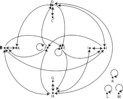
Figure 4: The graph for the set of all points made up of constant blocks which will add a consistent ${\bf y}$ at each time step. See Table 3 for definitions of A,B,C,D,E,F,G,H,I,J,K,L,M.

Note that the set $\mathcal{G}$ defined in Section 3.1 is contained in $\mathcal{G}^{*}$. Note also that $\mathcal{G}^{*}$ is closed and $\Gamma$-invariant. An interesting question is whether $\mathcal{G}^{*}$ is an attractor set for the sand automaton $\Gamma$. We have conducted simulations where the space time diagrams of several initial configurations are generated. Empirically what seems to be happening is that the iterates of the initial configuration converge “almost everywhere” to a configuration in $\mathcal{G}^{*}$. We describe what we mean by this: define the words $O={{-2}\choose{-2}}{{2}\choose{0}}{{0}\choose{2}}{{-2}\choose{-2}},P={{-2}\choose{-1}}{{1}\choose{0}}{{0}\choose{1}}{{-1}\choose{-2}}$ and $Q={{2}\choose{2}}{{-2}\choose{0}}{{0}\choose{-2}}{{2}\choose{2}},R={{2}\choose{1}}{{-1}\choose{0}}{{0}\choose{-1}}{{1}\choose{2}}$. These sets of words are 2-periodic in the sense that if $f\circ\Pi(\Phi^{n}(\textbf{x})_{[i,i+3]})=O$ then $f\circ\Pi(\Phi^{n+1}(\textbf{x})_{[i,i+3]})=P$ and if $f\circ\Pi(\Phi^{n}(\textbf{x})_{[i,i+3]})=Q$ then $f\circ\Pi(\Phi^{n+1}(\textbf{x})_{[i,i+3]})=R$. If we include these in a new graph ${\mathcal{H}}^{\prime}$, then this seems to describes the asymptotic behaviour of $\Phi$ more accurately. The graph ${\mathcal{H}}^{\prime}$ is presented in Figure 5. This leads to the following conjecture. Similar to our definition of ${\mathcal{G}}^{*}$, let

$$\mathcal{G}^{\prime}:=\{{\bf x}:f(\Pi({\bf x}))\mbox{ corresponds to an infinite path in }{\mathcal{H}}^{\prime}\}.$$

Conjecture 4.10.

The set $\mathcal{G}^{\prime}$ is an attractor for $\Gamma$, in that if ${\bf x}\in X$, then $\lim_{n\rightarrow\infty}d(\Gamma^{n}(x),\mathcal{G}^{\prime})=0$.

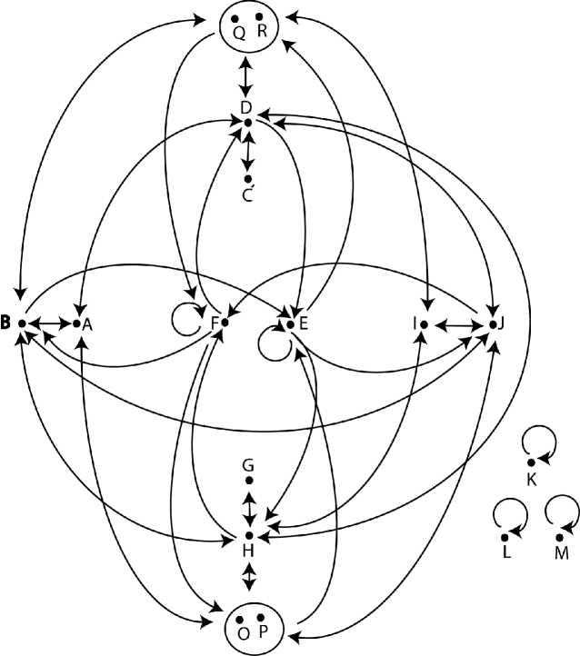
Figure 5: A potential attractor set for $\Gamma$.

References

- [BBC+92] J. Banks, J. Brooks, G. Cairns, G. Davis, and P. Stacey. On Devaney’s definition of chaos. Amer. Math. Monthly, 99(4):332–334, 1992.
- [BTW88] Per Bak, Chao Tang, and Kurt Wiesenfeld. Self-organized criticality. Phys. Rev. A (3), 38(1):364–374, 1988.
- [CFM07] Julien Cervelle, Enrico Formenti, and Benoît Masson. From sandpiles to sand automata. Theoret. Comput. Sci., 381(1-3):1–28, 2007.
- [CFMM97] Gianpiero Cattaneo, Enrico Formenti, Giovanni Manzini, and Luciano Margara. On ergodic linear cellular automata over . In STACS 97 (Lübeck), volume 1200 of Lecture Notes in Comput. Sci., pages 427–438. Springer, Berlin, 1997.
- [CM96] Bruno Codenotti and Luciano Margara. Transitive cellular automata are sensitive. Amer. Math. Monthly, 103(1):58–62, 1996.
- [DGM09] Alberto Dennunzio, Pierre Guillon, and Benoît Masson. Sand automata as cellular automata. Theoret. Comput. Sci., 410(38-40):3962–3974, 2009.
- [Hed69] G. A. Hedlund. Endormorphisms and automorphisms of the shift dynamical system. Math. Systems Theory, 3:320–375, 1969.
- [IÔN83] Masanobu Itô, Nobuyasu Ôsato, and Masakazu Nasu. Linear cellular automata over . J. Comput. System Sci., 27(1):125–140, 1983.
- [MM98] Giovanni Manzini and Luciano Margara. Invertible linear cellular automata over : algorithmic and dynamical aspects. J. Comput. System Sci., 56(1):60–67, 1998.