Buildup of Magnetic Shear and Free Energy During Flux Emergence and Cancellation

Abstract

We examine a simulation of flux emergence and cancellation, which shows a complex sequence of processes that accumulate free magnetic energy in the solar corona essential for the eruptive events such as coronal mass ejections (CMEs), filament eruptions and flares. The flow velocity at the surface and in the corona shows a consistent shearing pattern along the polarity inversion line (PIL), which together with the rotation of the magnetic polarities, builds up the magnetic shear. Tether-cutting reconnection above the PIL then produces longer sheared magnetic field lines that extend higher into the corona, where a sigmoidal structure forms. Most significantly, reconnection and upward energy-flux transfer are found to occur even as magnetic flux is submerging and appears to cancel at the photosphere. A comparison of the simulated coronal field with the corresponding coronal potential field graphically shows the development of nonpotential fields during the emergence of the magnetic flux and formation of sunspots.

1 Introduction

Regions of intense solar magnetic fields such as sunspots and active regions are known to exhibit energetic outbursts that are manifest in many forms, such as CMEs, filament eruptions, and flares (e.g. Forbes, 2000; Low, 2001; Forbes et al., 2006; Gopalswamy, 2006; Schrijver, 2009). In the most dramatic form, magnetic fields release energy up to $10^{32}$ ergs, and in the process expels $10^{15}$ gm of plasma and $10^{20}$ Mx of magnetic flux into interplanetary space (Bieber & Rust, 1995) at speeds that can reach 3000 km/s (e.g. Gosling et al., 1990; St. Cyr et al., 2000; Zhang et al., 2004). Although less energetic, large-scale regions of relatively weak magnetic fields can also erupt giving rise to streamer blowouts and the expulsion of quiescent filaments into the solar wind (e.g. Hundhausen, 1993; Lynch et al., 2010).

In order to produce such eruptions, the magnetic field must possess free magnetic energy, which requires that the field is in a nonpotential configuration with electric currents passing through the photosphere and into the corona. In general, the field lines of the non-potential force-free fields are stretched, expanded and intertwined compared to the equivalent potential field mapping to the photosphere. Such force-free fields in the solar corona have historically been taken to be of two forms: arcades, in which the foot points have been sheared to produce a strong field component parallel to the polarity inversion line (PIL), or flux ropes, in which the magnetic field is twisted about a central axis. This dichotomy of field configurations naturally leads to two broad groups of theoretical and numerical models of CMEs.

In the case of magnetic arcades, initial configurations are typically taken to be line-tied to the lower boundary and subsequently energized with prescribed shear flows, which cause the arcade to expand and then erupt (e.g. Steinolfson, 1991; Mikic & Linker, 1994; Amari et al., 1996; Guo & Wu, 1998). Another variant, the so-called breakout model, involves a system of quadrupolar fields with a system of three arcades. The field reverses direction over the central arcade allowing magnetic reconnection to release the central arcade (e.g. Antiochos et al., 1999; Lynch et al., 2004, 2008; van der Holst et al., 2009). In all of these cases, magnetic flux ropes form during the eruption process and are expelled from the corona. For those models, which assume that flux ropes exist prior to the eruption, the flux ropes are assumed to reside within an arcade where the outward-directed Lorentz force of the rope (hoop force) is balanced by magnetic tension of the surrounding arcade (e.g. Forbes & Isenberg, 1991; Low, 1994; Titov & Démoulin, 1999). The central question with flux rope models is how the force imbalance occurs and results in eruption. Flux ropes have been energized by the application of rotational motions at the rope footpoints (e.g. Tokman & Bellan, 2002; Rachmeler et al., 2009) that twist up the field. Flux ropes have also been forced to emerge into the corona by bodily advecting them through the lower boundary of the computational domain (e.g. Török & Kliem, 2005; Fan, 2005). In the case of Amari et al. (2003), flux cancellation at the PIL forms a flux rope within a sheared magnetic arcade. Following these formation processes, the flux rope may lose equilibrium and erupt from several instabilities including: unbalance of magnetic forces, which is followed by magnetic reconnection (Forbes & Isenberg, 1991; Amari et al., 2003; Roussev et al., 2004), torus instability (Török & Kliem, 2005), or kink instability (Sturrock et al., 2001; Fan, 2005).

Plentiful observations provide evidence for both arcades and flux ropes as the coronal field structures for CMEs. Sheared magnetic fields are measured directly at the photosphere with vector magnetographs (e.g. Hagyard et al., 1984; Zirin & Wang, 1993; Falconer, 2001; Yang et al., 2004; Liu et al., 2005), where the field is found to run nearly parallel to the PIL. More recent analysis by Schrijver et al. (2005) found that shear flows associated with flux emergence drove enhanced flaring. Similarly, active region CME productivity is also strongly correlated with magnetic shear, as shown by Falconer et al. (2002, 2006). There is also evidence suggesting that flux ropes may bodily emerge through the photosphere to reside in the corona. The twist of the emerging flux tube is characterized by the presence of elongated magnetic polarities, i.e., magnetic tongues in longitudinal magnetograms (Luoni et al., 2011). Leka & Steiner (2001) examined a time series of vector magnetograms of emerging magnetic flux and found that magnetic fields passing through the photosphere are already twisted. Similarly, Lites et al. (1995) examined a time series of photospheric vector magnetograms, which they found could be fitted by the emergence of a spherically shaped magnetic flux rope. Lites (2005) shows an example of the photospheric vector magnetic field and chromospheric structure seen in the H$\alpha$ line, which suggest the presence of a coronal flux rope associated with a prominence.

Magnetohydrodynamic (MHD) numerical simulations may provide new insights to our understanding of the physical processes that build up the free magnetic energy necessary for solar eruptions. Global scale simulations address how magnetic fields generated at the tachocline pass through the convection zone and have explained and reproduced many large-scale aspects of sunspots (e.g. Spruit & van Ballegooijen, 1982; Abbett et al., 2001; Fan, 2008). However because of the anelastic approximation, these models can only extend up to a height of 20 Mm below the photosphere. Above this depth, fully compressible MHD models have been employed to simulate the emergence of magnetic fields from the near surface convection zone into the lower corona. Early work demonstrated the basic processes by which fields emerge to form bipolar active regions (e.g. Shibata et al., 1989; Matsumoto et al., 1993). These simulations were followed by cases (e.g. Manchester, 2001; Fan, 2001; Magara & Longcope, 2003), which showed that the Lorentz force, arising when fields expand into the highly stratified solar atmosphere, drives shear flows along the PIL. The shear flows then transport magnetic energy into the coronal portion of the flux rope which then expands, and drive its eruption (Manchester et al., 2004). This shearing process is suggested as the energy source for CMEs and flares (Manchester, 2007, 2008). Galsgaard et al. (2007), Archontis & Török (2008), and MacTaggart & Hood (2009) produce fast CME-like eruptions by also invoking magnetic reconnection with emerging flux ropes. Fan (2008) simulated flux rope emergence that exhibited sunspot rotation driven by a torsional form of the Lorentz force, which twisted up the coronal portion of the field as predicted by Parker (1977). However, in this case, no eruptive behavior was found.

Recently, computing power has reached a level that has allowed the development of realistic solar models, including radiative and thermodynamic processes necessary to simulate convection in conjunction with the upper atmosphere. Stein & Nordlund (2006), Abbett (2007), Rempel et al. (2009), Cheung et al. (2010), Kitiashvili et al. (2010), and Rempel (2011) emphasize the importance of the interaction between magnetic fields and convective motions. Stein & Nordlund (2006) and Abbett (2007), have each addressed quiet-Sun magneto-convection, while Kitiashvili et al. (2010) report the critical role of strong vortical downdrafts around small magnetic structures in the formation of large-scale structures. The work of Rempel et al. (2009) and Cheung et al. (2010) treats the formation and evolution of sunspots, including the Evershed flow. Fang et al. (2010, 2012) address the emergence of magnetic flux ropes from a turbulent convection zone into the corona and found both shearing and rotational flows driven by the Lorentz force. These horizontal flows were found to dominate the energy transport from the convection zone into the corona. Of particular significance, the simulation of Fang et al. (2012) exhibited a case of large-scale flux cancellation, a phenomena strongly associated with CME initiation (Subramanian & Dere, 2001). Here we examine the flux cancellation in conjunction with energy transport from the convection zone to the corona.

The paper is organized in the following way: Section 2 describes the numerical simulation; Section 3 studies the build up of magnetic shear in a flux cancellation event; followed by analysis on the free energy in the corona in Section 4. The energy transfer at the photosphere is discussed in Section 5. Section 6 summarizes our conclusions and discussion.

2 Numerical Simulation

To simulate the flux emergence in the convection zone, we first generate a relaxed solar atmosphere of dimension $30\times 30\times 42$ Mm³, with the photosphere located at $Z=$ 0 Mm. Our model solves the MHD equations in Block-Adaptive Tree Solar-wind Roe Upwind Scheme (BAT-S-RUS) with additional energy source terms to describe thermodynamic processes in the solar atmosphere, i.e., radiative cooling at the photosphere and in the corona, and coronal heating (Abbett, 2007; Fang et al., 2010). Meanwhile, implementation of the non-ideal tabular equation-of-state (Rogers, 2000) provides a more accurate description of the partially ionized plasma in the convection zone. We use periodic horizontal, closed upper boundary conditions, and fix the density and temperature values at the lower boundary while setting the vertical momentum to be reflective.

Taking advantage of the adaptive grid in BAT-S-RUS, our model produces a relaxed convection zone with a depth of 20 Mm, with a overlying photosphere of 0.45 Mm thickness and a corona of 20 Mm, in a Cartesian domain. The vertical statification of the atmosphere in our simulation domain is shown in Figure 1 in Fang et al. (2012). We then carry out a simulation of the emergence of a buoyant, initially stationary, horizontal flux rope inserted at $Z=-10$ Mm, shown in Figure 2 in Fang et al. (2012). Interaction of the rising flux rope with large-scale convective motion produces the bipolar structure of the flux rope, with the convective downflows fixing the two ends of the emerged section of the flux rope in the convection zone, illustrated in Figure 5 in Fang et al. (2012). Near-surface small-scale convection produces the magnetic polarities by coalescence and intensifies the strength of the magnetic flux. A small active region forms on the photosphere, seen in Figure 6 of Fang et al. (2012), exhibiting strong interaction of the magnetic flux and the surface flows, i.e., the shearing and converging motions, separation and rotation of the magnetic polarities. In the presence of these flows, a flux cancellation event takes place at time t = 05:00:00, shown by Figure 6 of Fang et al. (2012), during which 10% of the total photospheric unsigned flux is cancelled. During the flux emergence, horizontal motions dominate the energy transfer to the corona, while vertical flows transport energy back into the convection zone. Details on the dynamics of the emerging flux rope are discussed in Fang et al. (2012).

3 A case of Flux Cancellation

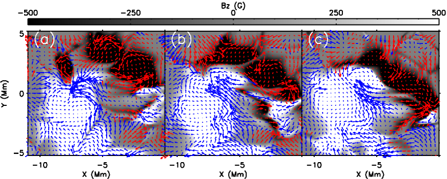
(a)

(b)

(c)

Figure 1: The photospheric structure of B_z in the area of flux cancellation at time t = 5:00:00 (a), 5:10:00 (b), 5:22:00 (c). Blue and red arrows show the horizontal velocity in positive and negative magnetic polarities, respectively. Shear flows are most apparent at time t = 5:10:00.

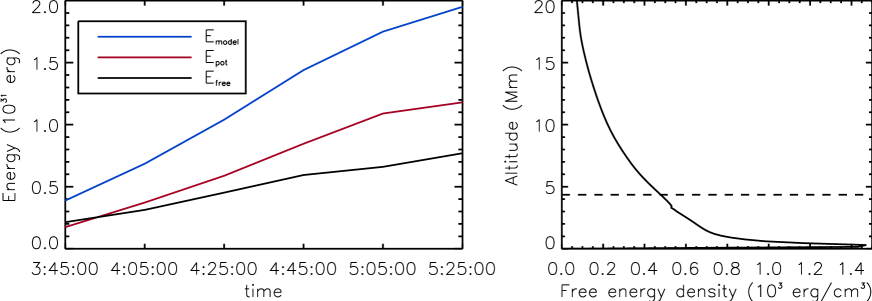
Figure 2: Left: temporal evolution of the total (blue), potential (red) and free (black) magnetic energy. Right: vertical distribution of free energy density at time t = 05:05:00. The dashed line indicates the altitude up to where 50% of the coronal free energy is stored.

Here, we examine a region of magnetic flux cancellation at the photosphere in our simulation, which is also associated by high magnetic shear. Flux cancellation of this form is particularly significant as it has been observed to be associated with flares (Martin et al., 1985) and CMEs (Subramanian & Dere, 2001) in active regions. A clear example is observed in AR 10977, where reconnection at the PIL during flux cancellation forms a highly sheared arcade and sigmoidal structure that subsequently reforms after eruption (Green et al., 2011). Li et al. (2004) found converging flows consistent with flux cancellation in decaying and young active regions producing CMEs. Inspired by similar observations, converging motion and flux cancellation have been imposed as boundary conditions in MHD simulations to produce eruptions (Linker et al., 2003; Amari et al., 2003).

As it is observed on the Sun, flux cancellation is very ambiguous as it may be caused by submergence of $\Omega$-loops, emergence of U-loops, or magnetic cancellation by some dissipative process. Our simulation provides a unique opportunity to fully understand an example of flux cancellation in a way that is not possible through observations alone. We find flux cancellation occurs spontaneously between opposite polarities that are driven together by the convective flows near the photosphere. The temporal evolution of cancellation is shown in Figure 1a-1c, which show a zoom-in view of the relevant area, with background color showing photospheric B_z field. The horizontal motions in positive and negative polarities are shown by blue and red arrows, respectively. The flux cancellation event starts at time t = 05:00:00, lasts for 0.5 hr, and the total amount of cancelled flux approaches $1\times 10^{20}$ Mx, which is 10% of the total unsigned flux on the photosphere. It is remarkable that during the process of flux cancellation, the coronal free energy (shown in the left panel of Figure 2) is still increasing even though the photospheric magnetic flux is decreasing.

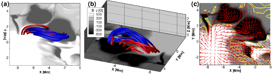
(a)

(b)

(c)

Figure 3: The structure of the magnetic fields in the area of flux cancellation at time t = 5:05:00 from top (a and c) and side (b) view. The background planes show the photospheric B_z field. Color on the rods indicates the vertical velocity at which the field lines are moving, with blue showing rising lines and red submerging. The red arrows in Panel (c) represent the horizontal magnetic field, with yellow line showing PIL.

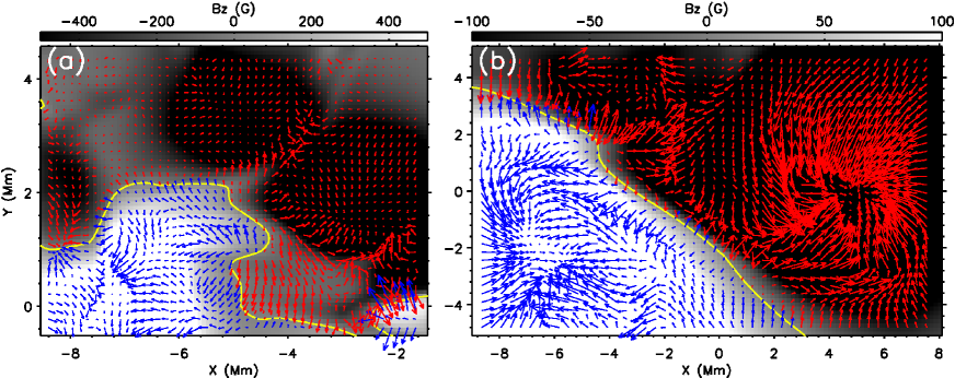
(a)

(b)

Figure 4: The structure of horizontal Lorentz force on Z = 0 (a) and Z = 3 Mm (b) planes at times t = 05:01:00 (a) and 05:05:00 (b), respectively. The blue and red arrows represent Lorentz forces in positive and negative polarities, respectively. The magnitude of $B_{z}$ field component is shown in gray scale. Note that the Lorentz force reverses direction across the polarity inversion line driving the shear flow, and forms a spiral pattern in the negative polarity driving a rotating flow.

To understand this process, we take a close examination of the velocity fields in the area of flux cancellation prior to, during and in the later phase of the event, as shown by Figure 1a, 1b and 1c, respectively. In Figure 1a, the two polarities are pushed together by the horizontal converging motion at the two sides of the PIL. The flow pattern at the PIL is mostly converging and forms a very narrow PIL at a later time illustrated in Figure 1b. Figure 1b shows a clear shearing motion at the PIL, with two polarities running in opposite directions. The strong shear flow at the PIL is driven by the Lorentz force, and takes place during the flux cancellation as the magnetic field expands in the corona as shown by the blue colored field lines in Figure 3a and 3b. Figure 4a shows the horizontal Lorentz force at time t = 05:01:00 with arrows, from which we find a clear pattern of the force running in the opposite directions across the PIL in the area of flux cancellation. At time t = 5:22:00, toward the end of the flux cancellation, the shearing motion is weakened and the flow pattern becomes dominated by the converging motion again, as shown in Figure 1c. The weak-strong-weak shearing motion in the flux cancellation event is also shown by observations (Su et al., 2007) during flares where footprints of the magnetic fields present the same pattern of motion.

Figure 3a - 3c show the configuration of the magnetic fields in the area of flux cancellation at time t = 05:05:00. Figure 3a provides the top view of the fields, and we find that instead of short loops perpendicular to the PIL, as is the case for potential fields, the field lines are instead elongated parallel to the PIL. Furthermore, the fields are more parallel to the PIL as they become closer to it, as shown by the red arrows in Figure 3c. At the photosphere, the magnetic fields are submerging to the convection zone at the PIL, as shown by the red rods in Figure 3b. The concentration of both the magnetic and velocity shear along the PIL demonstrates that the elongation of the field lines is the result of shearing motion, which is further enhanced by the converging motion at the PIL (Martens & Zwaan, 2001). These converging motions also gives rise to occurrence of tether-cutting reconnection close to the photosphere in the highly sheared fields as proposed by Moore et al. (2001) as an explanation for solar eruptive events. Figure 1 of Moore et al. (2001) envisioned reconnection inside a highly sheared core field, which would produce longer, nearly horizontal field lines higher in the corona, while at the base of the arcade, a system of short unsheared loops would form. This flux transfer process accumulates the free energy of the sheared field higher in the corona while at the same time reducing the magnetic tension by detaching the system from the photosphere. The rise of the arcade naturally leads to necking off of the fields, which in turn, promotes more reconnection. Unabated, the runaway reconnection provides a mechanism for the initialization and growth of explosive events. With our simulation, we can fully examine the way in which submergence and reconnection alter the field line geometry in the tether-cutting process. A three-dimensional (3-D) view of the magnetic fields combined with the flow pattern provides a complete picture of the effects of the internal reconnection. Figure 3b illustrates the structure of the magnetic field lines colored by the vertical component of the velocity orthogonal to the field lines. Blue indicates upflows and red downflows. We find two groups of magnetic field lines formed during tether-cutting reconnection, with one rising up into the corona and the other, shorter loops, submerging into the convection zone. At the photosphere, the submergence of the shorter loops, as shown by the red rods right above the PIL, results in the decreased unsigned flux observed at the surface. Along the long, rising loops, magnetic shear accumulates, forming a highly sheared arcade.

(a)

(b)

(c)

(d)

(e)

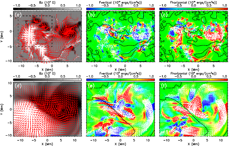
(f)

Figure 5: The structure of B_z (a and d), F_vertical (b and e) and F_emerge (c and f) fields at the photosphere (a, b and c) and at Z = 3 Mm in the corona (d, e, and f) at time t = 05:05:00. PIL is shown by the black line. Red arrows in Panel (a) and (d) represent the horizontal magnetic fields, and white arrows in (b, c, e and f) show the horizontal velocity fields.

To study the energy transport into the corona during flux cancellation, we examine the Poynting flux at $Z=3$ Mm associated with the vertical motions. At the surface, the vertical motion transports the energy back into the convection zone due to the concentration of the magnetic flux in downflows. In the corona, the acceleration of magnetic fields after reconnection plays a very important role in the energy flux, shown by Figure 5e. At the PIL in the corona, we observe a strong energy input associated with the rising motion of the fields. The rising motion here in the corona, however, is different from the emerging motion at the photosphere. At the photosphere, the emergence is caused by the expansion and buoyancy of the flux rope as well as convective upflows. However, in the corona, the tether-cutting reconnection forms longer loops possessing less magnetic tension, resulting in a magnetic pressure gradient force accelerating the magnetic fields upward.

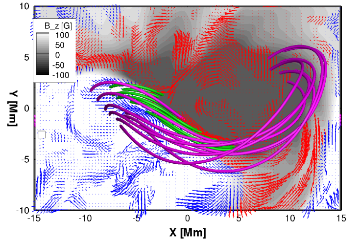
Figure 6: 3-D structure of the magnetic fields in corona at time t = 5:05:00. The background planes show the B_z field at Z = 3 Mm. Green rods represent low-lying field lines below 5 Mm with purple showing high field lines. The blue and red arrows show the horizontal velocity in positive and negative magnetic polarities, respectively. There is a clear shear flow along the polarity inversion line. The negative polarity also shows some signs of rotation, while the positive polarity shows only a coherent shear flow. The magnetic field lines clearly reflect the flow pattern.

Besides reconnection and shear flows, rotation of the magnetic polarities also contributes to the accumulation of magnetic shear by moving the footpoints in opposite directions at the PIL. Figure 6 shows the geometry of two groups of coronal magnetic field lines: purple overlying lines with apex higher than 5 Mm, and green lines lower than 5 Mm. Horizontal velocity fields at $Z=3$ Mm, represented by the arrows, show a rotation pattern on the negative polarity, which is also seen in Figure 5e. The rotation complements the shearing motion at the PIL, in the sense that both shear and rotation contribute to plasma motions parallel to the PIL. However the flow patterns are also quite distinct occurring at different scales and at different times. The shear flows are localized to the PIL and persist even when there is not a coherent rotation pattern in the magnetic polarities. When rotation is present, the shear flow tends to be greater in magnitude and will be shown graphically to dominate the energy transport into the corona.

The combination of the two motions creates a highly sheared arcade at the PIL, shown by the green rods in Figure 6, and rotation produces the twisted field structure at the far ends of the emerged fields, shown by purple rods. Both motions are driven by Lorentz force, as shown by the arrows in Figure 4b. At the PIL, the horizontal Lorentz force runs in the opposite direction, consistent with the directions of the shearing motion. In the negative polarity, the Lorentz force rotates in the same way of the rotation of the polarity. The sigmoidal structure at the PIL is maintained by the consistent shearing and rotating motions in our simulation. The relative contribution of shear flows compared to rotation can be seen in the geometry of the coronal fields at the PIL. Here, the field is dominated by an arcade structure instead of a twisted flux rope. Most of the twist is located at the outer periphery of the two polarities. Even in the most twisted field lines, there is less than a full turn of the field around the axis of either polarity. The absence of the twisted flux rope may be explained by two facts: the axis of the initial magnetic flux rope remains in the convection zone; and there are not enough twisting motions on the surface to reproduce such a twisted structure after emergence. The emerged fields are sheared and elongated, forming the arcade structure over the PIL.

4 Non-potentiality of the Magnetic Field

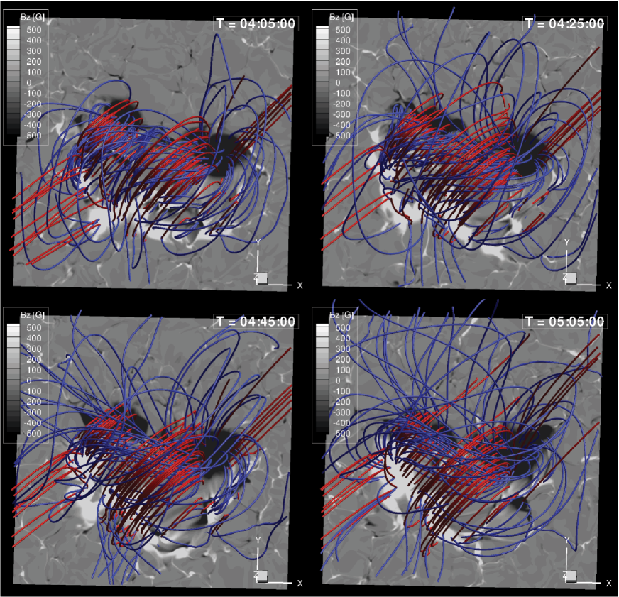
Figure 7: Comparison of the model field (blue) with the extrapolated potential field (red) at time t = 04:05:00, 04:25:00, 04:45:00 and 05:05:00. The color on the plane shows the B_z field at the photosphere. The clearest departure in field line direction occurs at the sheared field lines above the PIL.

During our simulation, a significant amount of energy, up to 2$\times 10^{31}$ ergs, is transferred into the corona, over 5 hours of evolution. The question is then, how much of the magnetic energy is in a free form, which is necessary for solar eruptive events. To investigate the evolution of magnetic free energy, we compare the coronal magnetic fields in our simulation with potential fields extrapolated from the photospheric boundary conditions. Figure 7 shows the temporal evolution of the model fields (blue) and the extrapolated potential fields (red). Comparison between the two fields clearly shows the buildup of magnetic shear along the field lines during the process of flux emergence. At time t = 04:05:00, shown by the upper-left panel in Figure 7, the magnetic flux concentrates in two polarities, with most of the field lines running perpendicular to the PIL. The energy transfer into the corona occurs as the magnetic field lines become elongated and sheared along the PIL. The lower-right panel in Figure 7 shows the field structure at time t =05:05:00, in which the field lines are sheared along the PIL and compressed into the lower atmosphere while the overlying fields remain almost potential. The simulated configuration of the magnetic fields in our domain is consistent with observations and simulations of the magnetic fields before solar eruptions (Schrijver et al., 2008; Leake et al., 2010). The overlying fields confine and compress the sheared core in the lower atmosphere, which may be destabilized and give rise to sudden release of magnetic free energy.

(a)

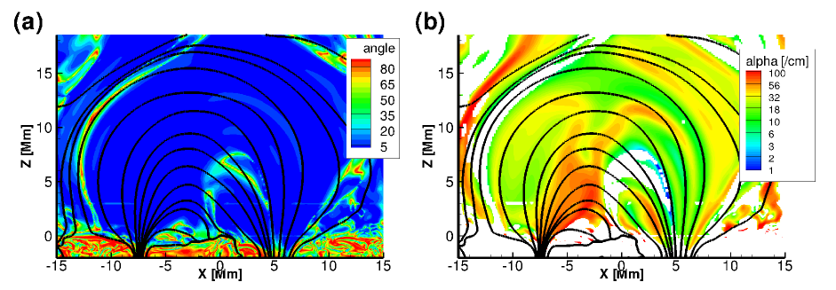
(b)

Figure 8: (a) the angle between the current and magnetic fields (b) the $\alpha$ structure on the Y = 0 plane. Black lines are the magnetic field lines and white regions in Panel (b) are areas where the angle between the current and magnetic fields are greater than $10^{\circ}$.

Here, we calculate the free energy for the simulation by integrating the magnetic energy for the model and subtracting the energy of the potential field. The results are shown in the left panel of Figure 2 where the temporal evolution of model, potential and free energy is plotted with blue, red and black lines, respectively. Beginning at time t = 04:05:00, the amount of free energy doubles within one hour (the period shown by Figure 7), such that the coronal free energy approaches $7\times 10^{30}$ ergs while the total energy is $1.7\times 10^{31}$ ergs. At this time, the free energy contributes to 40% of the total energy. Meanwhile, the vertical stratification of the free magnetic energy, is shown in the right panel of Figure 2. The line plot shows a strong tendency of concentrating free energy in the lower atmosphere, with 50% located below $Z=4$ Mm, shown by the dashed line. Figure 8a and 8b shows the angle between the current and the magnetic field and the structure of $\alpha$ (the ratio of $|4\pi\mathbf{j}|$ and $|\mathbf{B}|$ when the angle between them is less than 10^∘) in the Y = 0 plane, respectively. The non-force-free magnetic fields, as shown in Figure 8a mainly reside in the convection zone, the core sheared field close to the surface and the negative polarity where the rotation forms a twisted magnetic structure (see Figure 7). Note that $\alpha$ tends to be maximized low down the center of the arcade structure and then falls off with distance from the PIL.

5 Poynting Fluxes

To separate the energy transfer associated with vertical and horizontal flows, we decompose the Poynting flux into two components:

$$F_{\mathrm{horizontal}} = -\frac{1}{4\pi}\left(B_{x}u_{x}+B_{y}u_{y}\right)B_{z},$$ (1)

$$F_{\mathrm{vertical}} = \frac{1}{4\pi}\left(B_{x}^{2}+B_{y}^{2}\right)u_{z}.$$ (2)

F_vertical indicates the energy transported by the vertical motion, while F_horizontal represents the energy flux due to the horizontal motions, which include, at the photosphere, the separation of small dipoles, rotation, and the shearing flow along the PIL. Figure 5b and 5c show the structures of F_vertical and F_horizontal, respectively, with the arrows representing the horizontal velocity fields. It is clear that in regions with rotation or shearing there is a strong energy input into the corona. Comparison of the structures of F_vertical and F_horizontal suggests that horizontal motion dominates in the energy transfer during the current phase of emergence, while vertical motion transfers energy back into the convection zone, due to the concentration of magnetic flux in downflow regions (Fang et al., 2010, 2012). Vertical emerging motion dominates at the very beginning of the flux emergence, and later gives way to horizontal motions, a pattern found earlier by Magara & Longcope (2003) and Manchester et al. (2004).

At the photosphere, the magnetic field is very highly structured by convection. In particular, the flow patterns and Poynting fluxes can be difficult to interpret with a large component of their structure being caused by random convective motions. To get a better understanding of the dynamics, we plot the vertical field strength, flow field and Poynting fluxes in the low corona at a height of $Z=3$ Mm in Figure 5d - 5f. Here, in the corona, the magnetic field expands and smooths out as the plasma beta drops. This transition allows us to make a much clearer picture of the relevant structures. The flux expands to form two nearby polarities and an elongated PIL between them, shown by Figure 5d. Here, the presence of a highly sheared field is obvious in the red arrows showing the horizontal field direction. The positive polarity shows little discernible twist while the negative polarity is clearly twisted. Flows are completely dominated by shearing motion at the PIL and rotation in the polarities. Both flows make a significant contribution to the energy transfer, but the energy transported by shear flow tends to be more consistent in time than that of rotational flows.

6 Summary and Conclusions

Our simulation provides us with a unique opportunity to study an example of magnetic flux emergence in a realistic simulation of the convection zone, coronal system. The system shows a wealth of complexity and interaction of mutiple physical processes, which conspire to transport magnetic flux and free energy from the convection zone into the corona. The emerging magnetic flux interacts with convective cells of varying scales as it approaches the photosphere, and then accumulates in convective downdrafts to form a bipolar magnetic structure resembling a solar active region. The magnetic field continually expands into the upper atmosphere, which results in shear flows and rotating motions that combine to draw the field nearly parallel to the PIL, and transport energy into the corona. At a later time, converging motions at the PIL cause flux cancellation at the photosphere along with tether-cutting reconnection, which produces highly sheared, sigmoidal shaped field lines high in the corona.

In the process of building up the magnetic free energy, shearing flows play a significant role at the photosphere and in the corona. At the near surface layers, the angle between the current and magnetic fields ranges from $35^{\circ}$ to $90^{\circ}$. The geometry of current and magnetic fields then produces the Lorentz force at the surface, which drives the rotating and shearing motions and increases the non-potentiality of the magnetic fields over a period of hours after the emergence. In particular, the shearing flows align the magnetic fields nearly parallel to the PIL and transport significant amount of magnetic energy from convection zone into the corona during the flux emergence, consistent with observations by Schrijver et al. (2005). The shearing flows at the PIL are accompanied by periods of rotating motion of the magnetic polarities. Both of the two motions contribute to the build up of magnetic shear and free energy in the corona. However, the shearing motions distinguish themselves from the rotation by their persistent presence and concentration at the PIL where the field has an arcade structure, while rotation on the other hand is only present in one of the magnetic polarities and lasts only for 1 hour. It is the long-lasting, Lorentz-force driven shearing motion that dominates the energy transfer.

Convection-driven converging motion drives flux bundles of opposite polarities together, producing strong magnetic gradient and the pronounced PIL, preferential for large flares (Schrijver, 2007; Falconer et al., 2008). The horizontal converging motion at the PIL also contributes to the development of the magnetic shear of the field lines by increasing the shear angle (Martens & Zwaan, 2001). The combination of converging and shearing flows at the PIL forms a group of highly sheared arcades overlying a sharp magnetic PIL. Within this arcade, converging motions lead to the occurrence of tether-cutting reconnection, producing two types of field lines: one long sheared expanding loops and the other unsheared submerging loops. The short loops sink into the convection zone at the speed of convective flows, up to 2 km/s, consistent with Harvey et al. (1999), which continuously reduces the photospheric unsigned flux. The longer loops rise into the corona with more magnetic shear. The shearing motion along the PIL plays a very important role in that it both produces a sheared arcade structure ready for reconnection and accumulates magnetic shear in the field lines formed after the reconnection. The magnetic configuration of this area thus yields a high free energy up to 40% of the total, which is comparable with the threshold value for eruptions reported by Amari et al. (2003), Aulanier et al. (2010) and Moore et al. (2012).

Shear flows, converging motions, and tether-cutting reconnection combine to continuously build up the magnetic shear and free energy in the corona necessary for eruptive and explosive events. The magnetic reconnection and shearing motion at the photosphere produce the sigmoid-shaped field geometry, which is preferential for CMEs (Canfield et al., 1999), and the persistent sheared arcade structure is consistent with many CME models (e.g. Steinolfson, 1991; Mikic & Linker, 1994; Amari et al., 1996; Guo & Wu, 1998; Antiochos et al., 1999). Futhermore, we find coronal free energy grows at a rate of $3\times 10^{30}$ ergs/hr, which builds up $10^{31}$ ergs free energy over 5 hours. Such a build up rate is observed by Schrijver (2007) prior to large flares. Moreover, the majority of the free energy resides low in the corona where it can be confined and later released by reconnection. Finally, we note that the consistent shearing motion and reconnection at the flux cancellation site keep reforming the sigmoid structure, which is essential for homologous eruptive events.

In our simulation here, tether-cutting reconnection and flux cancellation take place in the highly sheared magnetic fields along the PIL, in the presence of converging and shearing flows. In the coupled system of the convection zone, the photosphere and the corona, all these mechanisms combine to work simultaneously and build up the free magnetic energy in the coronal fields. More importantly, the resulting geometry of the magnetic fields in our domain consists of compact, highly sheared core fields confined by more relaxed, overlying fields. 50% of the corona free magnetic energy is stored within the compressed, sheared core, while the overlying fields relax very quickly with altitude. The compact core, possessing free magnetic energy up to 10³⁰ ergs, provides the preferential magnetic structure as well as free energy for solar eruptions. We expect that in future simulations of larger scales, shear flows, converging motion and reconnection will produce enough free magnetic energy and give rise to eruptions of the magnetic system.

References

- Abbett (2007) Abbett, W. P. 2007, ApJ, 665, 1469
- Abbett et al. (2001) Abbett, W. P., Fisher, G. H., & Fan, Y. 2001, ApJ, 546, 1194
- Amari et al. (2003) Amari, T., Luciani, J. F., Aly, J. J., Mikic, Z., & Linker, J. 2003, ApJ, 585, 1073
- Amari et al. (1996) Amari, T., Luciani, J. F., Aly, J. J., & Tagger, M. 1996, ApJ, 466, L39
- Antiochos et al. (1999) Antiochos, S. K., DeVore, C. R., & Klimchuk, J. A. 1999, ApJ, 510, 485
- Archontis & Török (2008) Archontis, V. & Török, T. 2008, A&A, 492, L35
- Aulanier et al. (2010) Aulanier, G., Török, T., Démoulin, P., & DeLuca, E. E. 2010, ApJ, 708, 314
- Bieber & Rust (1995) Bieber, J. W. & Rust, D. M. 1995, ApJ, 453, 911
- Canfield et al. (1999) Canfield, R. C., Hudson, H. S., & McKenzie, D. E. 1999, Geophys. Res. Lett., 26, 627
- Cheung et al. (2010) Cheung, M. C. M., Rempel, M., Title, A. M., & Schüssler, M. 2010, ApJ, 720, 233
- Falconer (2001) Falconer, D. A. 2001, J. Geophys. Res., 106, 25185
- Falconer et al. (2002) Falconer, D. A., Moore, R. L., & Gary, G. A. 2002, ApJ, 569, 1016
- Falconer et al. (2006) —. 2006, ApJ, 644, 1258
- Falconer et al. (2008) —. 2008, ApJ, 689, 1433
- Fan (2001) Fan, Y. 2001, ApJ, 554, L111
- Fan (2005) —. 2005, ApJ, 630, 543
- Fan (2008) —. 2008, ApJ, 676, 680
- Fang et al. (2010) Fang, F., Manchester, W., Abbett, W. P., & van der Holst, B. 2010, ApJ, 714, 1649
- Fang et al. (2012) Fang, F., Manchester, IV, W., Abbett, W. P., & van der Holst, B. 2012, ApJ, 745, 37
- Forbes (2000) Forbes, T. G. 2000, J. Geophys. Res., 105, 23153
- Forbes & Isenberg (1991) Forbes, T. G. & Isenberg, P. A. 1991, ApJ, 373, 294
- Forbes et al. (2006) Forbes, T. G., Linker, J. A., Chen, J., Cid, C., Kóta, J., Lee, M. A., Mann, G., Mikić, Z., Potgieter, M. S., Schmidt, J. M., Siscoe, G. L., Vainio, R., Antiochos, S. K., & Riley, P. 2006, Space Sci. Rev., 123, 251
- Galsgaard et al. (2007) Galsgaard, K., Archontis, V., Moreno-Insertis, F., & Hood, A. W. 2007, ApJ, 666, 516
- Gopalswamy (2006) Gopalswamy, N. 2006, Space Sci. Rev., 124, 145
- Gosling et al. (1990) Gosling, J. T., Bame, S. J., McComas, D. J., & Phillips, J. L. 1990, Geophys. Res. Lett., 17, 901
- Green et al. (2011) Green, L. M., Kliem, B., & Wallace, A. J. 2011, A&A, 526, A2+
- Guo & Wu (1998) Guo, W. P. & Wu, S. T. 1998, ApJ, 494, 419
- Hagyard et al. (1984) Hagyard, M. J., Teuber, D., West, E. A., & Smith, J. B. 1984, Sol. Phys., 91, 115
- Harvey et al. (1999) Harvey, K. L., Jones, H. P., Schrijver, C. J., & Penn, M. J. 1999, Sol. Phys., 190, 35
- Hundhausen (1993) Hundhausen, A. J. 1993, J. Geophys. Res., 98, 13177
- Kitiashvili et al. (2010) Kitiashvili, I. N., Kosovichev, A. G., Wray, A. A., & Mansour, N. N. 2010, ApJ, 719, 307
- Leake et al. (2010) Leake, J. E., Linton, M. G., & Antiochos, S. K. 2010, ApJ, 722, 550
- Leka & Steiner (2001) Leka, K. D. & Steiner, O. 2001, ApJ, 552, 354
- Li et al. (2004) Li, Y., Luhmann, J., Fisher, G., & Welsch, B. 2004, Journal of Atmospheric and Solar-Terrestrial Physics, 66, 1271
- Linker et al. (2003) Linker, J. A., Mikić, Z., Lionello, R., Riley, P., Amari, T., & Odstrcil, D. 2003, Physics of Plasmas, 10, 1971
- Lites (2005) Lites, B. W. 2005, ApJ, 622, 1275
- Lites et al. (1995) Lites, B. W., Low, B. C., Martinez Pillet, V., Seagraves, P., Skumanich, A., Frank, Z. A., Shine, R. A., & Tsuneta, S. 1995, ApJ, 446, 877
- Liu et al. (2005) Liu, C., Deng, N., Liu, Y., Falconer, D., Goode, P. R., Denker, C., & Wang, H. 2005, ApJ, 622, 722
- Low (1994) Low, B. C. 1994, Physics of Plasmas, 1, 1684
- Low (2001) —. 2001, J. Geophys. Res., 106, 25141
- Luoni et al. (2011) Luoni, M. L., Démoulin, P., Mandrini, C. H., & van Driel-Gesztelyi, L. 2011, Sol. Phys., 270, 45
- Lynch et al. (2008) Lynch, B. J., Antiochos, S. K., DeVore, C. R., Luhmann, J. G., & Zurbuchen, T. H. 2008, ApJ, 683, 1192
- Lynch et al. (2004) Lynch, B. J., Antiochos, S. K., MacNeice, P. J., Zurbuchen, T. H., & Fisk, L. A. 2004, ApJ, 617, 589
- Lynch et al. (2010) Lynch, B. J., Li, Y., Thernisien, A. F. R., Robbrecht, E., Fisher, G. H., Luhmann, J. G., & Vourlidas, A. 2010, Journal of Geophysical Research (Space Physics), 115, A07106
- MacTaggart & Hood (2009) MacTaggart, D. & Hood, A. W. 2009, A&A, 507, 995
- Magara & Longcope (2003) Magara, T. & Longcope, D. W. 2003, ApJ, 586, 630
- Manchester (2008) Manchester, W. 2008, in Astronomical Society of the Pacific Conference Series, Vol. 383, Subsurface and Atmospheric Influences on Solar Activity, ed. R. Howe, R. W. Komm, K. S. Balasubramaniam, & G. J. D. Petrie , 91–+
- Manchester (2001) Manchester, IV, W. 2001, ApJ, 547, 503
- Manchester (2007) —. 2007, ApJ, 666, 532
- Manchester et al. (2004) Manchester, IV, W., Gombosi, T., DeZeeuw, D., & Fan, Y. 2004, ApJ, 610, 588
- Martens & Zwaan (2001) Martens, P. C. & Zwaan, C. 2001, ApJ, 558, 872
- Martin et al. (1985) Martin, S. F., Livi, S. H. B., & Wang, J. 1985, Australian Journal of Physics, 38, 929
- Matsumoto et al. (1993) Matsumoto, R., Tajima, T., Shibata, K., & Kaisig, M. 1993, ApJ, 414, 357
- Mikic & Linker (1994) Mikic, Z. & Linker, J. A. 1994, ApJ, 430, 898
- Moore et al. (2012) Moore, R. L., Falconer, D. A., & Sterling, A. C. 2012, ApJ in press
- Moore et al. (2001) Moore, R. L., Sterling, A. C., Hudson, H. S., & Lemen, J. R. 2001, ApJ, 552, 833
- Parker (1977) Parker, E. N. 1977, ARA&A, 15, 45
- Rachmeler et al. (2009) Rachmeler, L. A., DeForest, C. E., & Kankelborg, C. C. 2009, ApJ, 693, 1431
- Rempel (2011) Rempel, M. 2011, ApJ, 729, 5
- Rempel et al. (2009) Rempel, M., Schüssler, M., & Knölker, M. 2009, ApJ, 691, 640
- Rogers (2000) Rogers, F. J. 2000, Physics of Plasmas, 7, 51
- Roussev et al. (2004) Roussev, I. I., Sokolov, I. V., Forbes, T. G., Gombosi, T. I., Lee, M. A., & Sakai, J. I. 2004, ApJ, 605, L73
- Schrijver (2007) Schrijver, C. J. 2007, ApJ, 655, L117
- Schrijver (2009) —. 2009, Advances in Space Research, 43, 739
- Schrijver et al. (2008) Schrijver, C. J., De Rosa, M. L., Metcalf, T., Barnes, G., Lites, B., Tarbell, T., McTiernan, J., Valori, G., Wiegelmann, T., Wheatland, M. S., Amari, T., Aulanier, G., Démoulin, P., Fuhrmann, M., Kusano, K., Régnier, S., & Thalmann, J. K. 2008, ApJ, 675, 1637
- Schrijver et al. (2005) Schrijver, C. J., De Rosa, M. L., Title, A. M., & Metcalf, T. R. 2005, ApJ, 628, 501
- Shibata et al. (1989) Shibata, K., Tajima, T., Steinolfson, R. S., & Matsumoto, R. 1989, ApJ, 345, 584
- Spruit & van Ballegooijen (1982) Spruit, H. C. & van Ballegooijen, A. A. 1982, A&A, 106, 58
- St. Cyr et al. (2000) St. Cyr, O. C., Plunkett, S. P., Michels, D. J., Paswaters, S. E., Koomen, M. J., Simnett, G. M., Thompson, B. J., Gurman, J. B., Schwenn, R., Webb, D. F., Hildner, E., & Lamy, P. L. 2000, J. Geophys. Res., 105, 18169
- Stein & Nordlund (2006) Stein, R. F. & Nordlund, Å. 2006, ApJ, 642, 1246
- Steinolfson (1991) Steinolfson, R. S. 1991, ApJ, 382, 677
- Sturrock et al. (2001) Sturrock, P. A., Weber, M., Wheatland, M. S., & Wolfson, R. 2001, ApJ, 548, 492
- Su et al. (2007) Su, Y., Golub, L., & Van Ballegooijen, A. A. 2007, ApJ, 655, 606
- Subramanian & Dere (2001) Subramanian, P. & Dere, K. P. 2001, ApJ, 561, 372
- Titov & Démoulin (1999) Titov, V. S. & Démoulin, P. 1999, A&A, 351, 707
- Tokman & Bellan (2002) Tokman, M. & Bellan, P. M. 2002, ApJ, 567, 1202
- Török & Kliem (2005) Török, T. & Kliem, B. 2005, ApJ, 630, L97
- van der Holst et al. (2009) van der Holst, B., Manchester, IV, W., Sokolov, I. V., Tóth, G., Gombosi, T. I., DeZeeuw, D., & Cohen, O. 2009, ApJ, 693, 1178
- Yang et al. (2004) Yang, G., Xu, Y., Cao, W., Wang, H., Denker, C., & Rimmele, T. R. 2004, ApJ, 617, L151
- Zhang et al. (2004) Zhang, J., Dere, K. P., Howard, R. A., & Vourlidas, A. 2004, ApJ, 604, 420
- Zirin & Wang (1993) Zirin, H. & Wang, H. 1993, Nature, 363, 426