Hubble Space Telescope Observations of an Outer Field in Omega Centauri: A Definitive Helium Abundance

Abstract

We revisit the problem of the split main sequence (MS) of the globular cluster $\omega$ Centauri, and report the results of two-epoch Hubble Space Telescope observations of an outer field, for which proper motions give us a pure sample of cluster members, and an improved separation of the two branches of the main sequence. Using a new set of stellar models covering a grid of values of helium and metallicity, we find that the best possible estimate of the helium abundance of the bluer branch of the MS is $Y=0.39\pm 0.02$.

For the cluster center we apply new techniques to old observations: we use indices of photometric quality to select a high-quality sample of stars, which we also correct for differential reddening. We then superpose the color-magnitude diagram of the outer field on that of the cluster center, and suggest a connection of the bluer branch of the MS with one of the more prominent among the many sequences in the subgiant region. We also report a group of undoubted cluster members that are well to the red of the lower MS.

1 Introduction

The stellar system $\omega$ Centauri (NGC 5139) is one of the most puzzling objects in our Galaxy. In an intriguing way, the large amount of attention devoted to this globular cluster has served to increase rather than decrease the number of mysteries that surround it. For several decades it had been recognized that the red giant branch (RGB) of $\omega$ Cen shows a spread in metallicity (Dickens & Woolley 1967, Cannon & Stobie 1973). The breadth in color of the RGB was interpreted as an indication of an intrinsic spread in chemical abundance, as subsequently confirmed by spectroscopic data (Freeman & Rodgers 1975); and Norris, Freeman, & Mighell (1996) suggested that two epochs of star formation have occurred. Today we know that there are many more populations than that (Lee et al. 1999, Pancino et al. 2000, Sollima et al. 2005, Villanova et al. 2007, Bellini et al. 2010, and references therein). It has been suggested further that at each metallicity there is a range in age (Sollima et al. 2005, Villanova et al. 2007).

More than a decade ago our group found that the main sequence (MS) of the cluster is double (Anderson 1997, 2002; Bedin et al. 2004). Because of the lack of information on the heavy elements in the MS components, the original version of Bedin et al. (2004) had proposed several explanations for the split, none of them conclusive. The referee, John Norris, strongly suggested, however, “TRY HELIUM”, in spite of the improbably high He abundance that would be required, and published his suggestion (Norris 2004).

The turning point was the work by Piotto et al. (2005), who actually measured the heavy elements along the two branches of the MS. They found that contrary to expectation, the bluer branch (bMS) has a higher rather than a lower metallicity than the redder branch (rMS), and that the only way to explain the photometric and spectroscopic results was that the helium abundance of the bMS is $Y\sim$ 0.4 — far beyond what its metallicity would imply. Very recently Dupree, Strader, & Smith (2011) have found direct evidence for an enhancement in He, from the analysis of the $\lambda$10830 transition of He I in the RGB stars of $\omega$ Cen. The correlation of He-line detection with [Fe/H], Al, and Na supports the assumption that He is enhanced in stars of the bMS. (It is still totally unclear, however, where a large enrichment of He could have come from, and how it could fit with current stellar-evolution models.)

In other clusters too, studies of the RGB (Bragaglia et al. 2010a) and of the HB (Gratton et al. 2010) have suggested a spread in He abundances. In both of these studies NGC 2808 has stood out especially as showing a clear spread in helium — not surprisingly, since that cluster has a main sequence that is split into three branches (Piotto et al. 2007). And in that cluster Pasquini et al. (2011) have used the He $\lambda$10830 line to estimate a helium value $Y\geq 0.39$, confirming suggestions by D’Antona & Caloi (2008) and by Bragaglia et al. (2010a); furthermore, Bragaglia et al. (2010b) have obtained spectra of MS stars on the reddest and on the bluest MS branches of NGC 2808, and find that abundances of individual heavy elements are very much in agreement with the scenario of normal He for the rMS and enhanced He for the bMS.

In the present paper we describe an outer field of $\omega$ Cen that has relatively few stars, but minimal crowding. This field has already been used in our paper on the splitting of the MS (Bedin et al. 2004), and also in a study of the radial behavior of the numbers of stars in the bMS and the rMS, by Bellini et al. (2009); the present paper is the fuller discussion that the latter authors promised for this field. In addition to our presentation of the MS split in this outer field, we sharpen our view of the central field, we fit theoretical isochrones to the two branches of the main sequence, and, importantly, we estimate the difference in their helium abundances, along with the quantitative uncertainty of that difference.

2 The Outer Field

2.1 Observations, Measurements, and Reductions

In the outer field (13^h 25^m 35$\fs$5, $-$47° 40′ 6$\farcs$7, same as the 17′ field in Bedin et al. 2004) we combined a new data set with an earlier one. We had already imaged this field, 17^′ from the center of $\omega$ Cen (core radius 1$\farcm$4, half-mass radius 4$\farcm$2, tidal limit 57^′), using the Wide Field Channel (WFC) of the Hubble Space Telescope’s (HST’s) Advanced Camera for Surveys (ACS). Those images (GO-9444, PI King), taken 3 July 2002, consisted of 2$\times$1300 s + 2$\times$1375 s with F606W, and 2$\times$1340 s + 2$\times$1375 s with F814W. Our follow-up program (GO-10101, PI King) was to have had second-epoch images in F814W only, but in view of the extreme interest ignited by the results presented in Bedin et al. (2004) and Piotto et al. (2005), we were able to get Director’s Discretion time that allowed us to repeat the F606W images as well. After a delay caused by a failed guide star, the second-epoch images were taken 24 Dec 2005, with exposures 2$\times$1285 s + 2$\times$1331 s in F606W and 4$\times$1331 s in F814W. Because of the delay, however, the orientation differed by 180 degrees. As we shall see, this change improved the photometry, but at the cost of somewhat complicating the astrometry.

The photometry was carried out using the procedures and software tools developed for the Globular Cluster Treasury program (Sarajedini et al. 2007), as described in detail by Anderson et al. (2008). We summarize here briefly: To each star image in each exposure we fit a point spread function (PSF) interpolated expressly for that star, using a 9 $\times$ 5 array of PSFs in each of the two chips of the ACS/WFC. These arrays model the spatial variation of the PSF, but for each individual exposure we add a “perturbation PSF” that fine-tunes the fitting to allow for small differences in focus, temperature, etc.

The fitting of each star uses its central 5 $\times$ 5 pixels, and yields a flux and a position. In addition we created a model of the extended outer parts of the PSF that allowed us to eliminate the artifacts that arise from outer features in the PSFs of bright stars, while excluding very few legitimate stars. (The PSFs are described in great detail in Anderson et al. 2008.)

We transformed our zero points to those of the WFC/ACS Vega-mag system following the procedure given in Bedin et al. (2005), and using the encircled energy and zero points given by Sirianni et al. (2005). Because of the high background ($\gtrsim$100 $e^{-}$ pixel^-1), combined with the fact that our exposures were taken at a time when inefficiencies in charge transfer were less serious than they are now, this field did not need any corrections for inadequate charge-transfer efficiency.

2.2 The Saturated Stars

Since the primary aim of the programs for which the images were taken had been the faint stars, neither of our epochs included short exposures. For the bright stars we had to derive the best photometry that we could from their saturated images. We used the method developed by Gilliland (2004), which works by recovering electrons that have bled into neighboring pixels. Our application of this method is described in Sect. 8.1 of Anderson et al. (2008). The method depends, however, on having a detector GAIN greater than 1. Unfortunately our first-epoch images were taken with GAIN=1, but in the second epoch we had GAIN=2 and were able to do effective photometry on the saturated images. Thus for saturated stars we had only the second epoch available.

Figure 1: (Left) The CMD as obtained from PSF fitting of unsaturated pixels. The horizontal dashed line marks the beginning of saturation in filter F606W. (Right) The same CMD, with photometry for saturated stars obtained as described in Sect. 2.2.

Because Gilliland’s method uses so different a procedure, we had to adjust the zero points of the magnitudes that it produced. The necessary shifts ($<0.02$ mag in each band) were easily determined from the stars in the 0.5-mag interval just below the saturation limit, where both methods are valid. Figure 1 shows the impressive improvement that the use of Gilliland’s method gave us for a stretch of about 3 magnitudes at the bright end. It also shows, however, that for stars brighter than $m_{\rm F606W}\sim 17.1$ even that method is unable to cope with saturation. (From the onset of saturation at magnitude 20.4 up to a magnitude about 17.1, however, there is a considerable improvement.)

2.3 Proper Motions

For the astrometry we did not need the elaborate procedures that we had used for the photometry; for our data set it was more appropriate simply to use the program described by Anderson & King (2006), to get position coordinates for each star in each _flt image. (These are the images that have been bias-subtracted and flat-fielded via the standard ACS pipeline, but have not been resampled; as such they are suitable for derivation of positions and fluxes by high-precision PSF-type analysis.)

Our next step was to apply the distortion corrections of Anderson (2002, 2006). We then needed to transform these positions into a common reference frame at each epoch, for which we arbitrarily chose one image at that epoch. For the transformations we selected among the brighter stars a set of stars that were in the main-sequence region of the color-magnitude diagram (CMD), so as to minimize any disturbing influence that inadvertent inclusion of field stars might have on our transformations.

Once we had all the positions in a single reference frame at each epoch, we measured the displacement of each star from the first epoch to the second, relative to a set of at least 10 of its immediate neighbors (dropping the few stars that did not have 10 near neighbors), so that each cluster star would have a near-zero displacement between the two epochs, while field stars would show noticeable motions.

Since the astrometry depends very little on the filter band, we were able to treat each filter the same, and combine the results. With a precision of better than 0.05 pixel for the coordinates of individual star images, the precision of a displacement from the mean of 8 exposures at each epoch should be 1/2 of that, so that over the 3.5-year baseline the proper motions should be good to 0.007 pixel per year, which for a 50-milliarcsec pixel is 0.35 mas yr^-1. Since the distance to $\omega$ Cen is about 5 kpc, this is equivalent to an uncertainty of $\sim 4$ km^-1 in the transverse motion of each star (appreciably less than the 10 km sec^-1 internal velocity dispersion of the cluster at this distance from the center [Merritt, Meylan, & Mayor 1997]). In practice, moreover, the field-star motions turn out to differ from the cluster motions by much more than the internal dispersion of the latter.

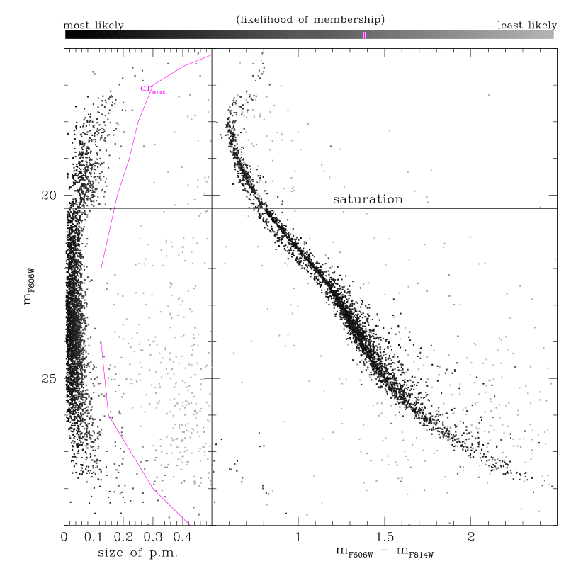
Figure 2: At left, the sizes of the proper motions (in pixel units), with the symbol for each star gray-scale-coded so as to show in an intuitive way the likelihood that it is a cluster member (as indicated in the palette at the top). The magenta lines in this panel and in the palette show our proper-motion cut-off for membership. In the right hand panel is the CMD of the same stars, with the same gray-scale coding, so that one can see the membership likelihood of each star in the CMD.

2.4 The Cleaned Color-Magnitude Diagram of the Outer Field

Because this field is so far from the center of $\omega$ Cen, it suffers relatively greater contamination by field stars than inner fields do; we therefore made careful use of proper motions to remove field stars from our color-magnitude diagram. Our first step was to plot the $x$ and $y$ components of proper motion for each unit interval of magnitude. From these plots it was clear that most of the motions — those of cluster members — were concentrated around a common centroid, while the motions of field stars scattered much more widely about another center. For bright stars there was little or no overlap between the two distributions, but with increasing measurement error at faint magnitudes the separation became less clear.

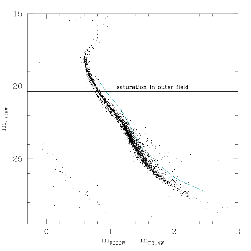
Figure 3: The color-magnitude diagram of cluster members in the outer field (stars whose proper motions lie to the left of the magenta line in the preceding figure). The dashed blue line marks the locus of equal-mass rMS binaries, 0.75 mag above the rMS.

In the left-hand panel of Figure 2 we show the sizes of the motions as a function of magnitude. We drew an arbitrary line, shown in magenta, to separate members from non-members. Rather than just throwing away the stars that we call non-members, however, we have colored each star from black to gray according to the palette shown at the top of the figure. Stars whose motions are very close to that of the cluster centroid are black; with increasing difference from the mean cluster motion the symbols become a paler and paler gray.

With the likelihood that each star is a cluster member coded in this intuitive way, in the right-hand panel of the figure we plot the stars in the color-magnitude diagram. The symbol that represents each star now has the same degree of grayness that the star was assigned in the left-hand panel, so that we can see where in the CMD the cluster members and the non-members lie, and conversely, from the gray level of the symbol, which stars should be rejected as non-members. Finally, in Figure 3 we show the CMD of the stars whose proper motions lie to the left of the magenta line in the preceding figure, which we therefore consider to be cluster members. The dashed blue line, 0.75 mag above the rMS, marks the upper limit of its binaries (those with equal mass).

As we have already noted, the flaring out of the MS at magnitudes brighter than 17 is due to the inability of our methods to cope with the most extreme levels of saturation. This anomaly aside, our CMD shows a number of interesting features: (1) The main sequence shows the best separation of its two branches that has yet been seen. (It should be noted that Fig. 3 is similar to Fig. 1(d) of Bedin et al. 2004, but now the interfering field stars have been removed. For the relative number of rMS and bMS stars one should see Bellini et al. 2009, whose study of the radial variation of the rMS/bMS ratio includes the results whose details we present here.) Also, in the following Section we will use the distance between the bMS and the rMS to derive a definitive value for the helium abundance of the bMS. (2) The bMS appears to cross over the rMS and emerge on the other side of it, in the subgiant region; we will discuss this further in Section 5. (3) A part of the white-dwarf sequence can be seen at the lower left (but we will not discuss it in this paper). (4) A considerable number of undoubted cluster members lie too far above and to the redward of the MS to be interpreted as binaries. Although they suggest some sort of sequence, their region is too ill defined to be called a sequence. This group too we will discuss in Sect. 5, in conjunction with the CMD of the much richer central region of the cluster.

3 The helium abundance of the bMS

Ever since the surprising discovery that the bMS has higher metallicity than the rMS (Piotto et al. 2005, P05), it has become increasingly evident that this reversal of the usual color progression with MS metallicity must indicate that the stars of the bMS contain a higher proportion of helium. Here we apply theoretical models of stellar structure to the question of what helium abundance the location of the observed blue sequence actually implies.

3.1 Fitting the color separation of the bMS and the rMS

For the comparison of observation with theory we select a single salient characteristic of the bifurcation of the main sequence: the color separation between the two branches. We measure this at a magnitude where the separation is large and the photometry is also quite reliable. Examining Fig. 3, we see that within the magnitude range in which our photometry is free from saturation the separation of the two sequences appears to remain nearly constant over a stretch of about two magnitudes, giving us a large enough number of stars to get a good value of the color separation of the two sequences. We will refer to this separation as $\Delta C$. Specifically, we chose the magnitude interval $20.6\leq m_{\rm F606W}\leq 21.8$, so that we can consider our observed $\Delta C$ to apply to the entire middle part of this range, i.e., for several tenths of a magnitude on either side of the midpoint, $m_{\rm F606W}=21.2$.

For the actual determination of the color separation we made use of a procedure that is described in great detail by Bellini et al. (2009). Briefly, we drew a fiducial color sequence along the gap between the two branches, and made the sequences approximately vertical by subtracting from the color of each star the fiducial color at its magnitude. We then plotted a histogram of the resulting colors, and fitted it with a pair of Gaussians. The separation that we find is $0.057\pm 0.0017$ mag, where the uncertainty is due only to the Poisson statistics of the star numbers in the two sequences. As a more conservative figure, however, we prefer to assign a three-sigma uncertainty, and to quote a color separation of $0.057\pm 0.005$.

For calculation of theoretical values of $\Delta C$ we chose absolute magnitude 7.0. For our distance modulus we took $(m-M)_{0}=13.70$ (Del Principe et al. 2006), $E(B-V)=0.12$ (Harris 2010), and $A_{V}=3.1\,E(B-V)$ (Cardelli et al. 1989); these give $(m-M)_{V}=14.072$, which we rounded to 14.1, so that $M_{\rm F606W}=7.0$ corresponds to $m_{\rm F606W}=21.1$, close to the middle of the magnitude range that we used for our observational $\Delta C$. (We note that the results that we derive below are insensitive to our exact choice of distance modulus, since the bMS and rMS run so closely parallel at these magnitudes.)

We wished to compare theoretical isochrones with the whole stretch of main sequence that is shown in Figure 3, and we therefore extended our models to lower masses ($M<0.5\,M_{\odot}$). We again took [$\alpha$/Fe] = +0.4, and used the physical scenario described by Pietrinferni et al. (2004, 2006). For these low masses, we rely on the equation of state by Saumon, Chabrier, & van Horn (1995) for dense, cool matter, and on low-temperature opacities by Ferguson et al. (2005) and high-temperature opacities by Rogers & Iglesias (1992). The outer boundary conditions were fixed by adopting the Next Generation model atmospheres provided by Allard et al. (1997) and Hauschildt et al. (1999a,b). We fixed the base of the atmosphere at Rosseland optical depth $\tau=100$, i.e., deep enough for the diffusion approximation to be valid. We note also that although detailed atmospheres are available only for canonical He abundances, helium does not appreciably affect the atmosphere, because its only effect would be on pressure-induced H₂–He absorption, which matters only in stars of lower mass than we discuss here (F. Allard, private communication). At any given metallicity, the match between the more massive models and the low-mass ones was made at a mass level where the transition in luminosity and effective temperature between the two regimes is smooth (usually $\sim 0.5\,M_{\odot}$).

We computed stellar models for [Fe/H] = $-$1.62 and $-$1.32, to represent the rMS and bMS respectively; and to allow for the uncertainty of 0.2 dex in the relative metallicities of the bMS and the rMS we also computed models with [Fe/H] = $-$1.52 and $-$1.12, to represent alternative [Fe/H] values for the bMS. For each value of [Fe/H] for the bMS, we calculated models for a set of helium abundances that reached beyond $Y=0.4$. Within the heavy elements we used the $\alpha$-enhanced mixture of Pietrinferni et al. (2006).

For the transformation of the theoretical stellar models into the observational plane we used the semi-empirical colors and bolometric corrections of Pietrinferni et al. (2004), transformed according to Appendix D of Sirianni et al. (2005). We also verified, however, that using the color–$T_{\rm eff}$ relations and bolometric corrections of Hauschildt et al. (1999a,b) would produce practically the same result. (In any case, whatever inaccuracies there may be in our transformation are greatly reduced by the fact that the quantity that we use is the difference between two colors.)

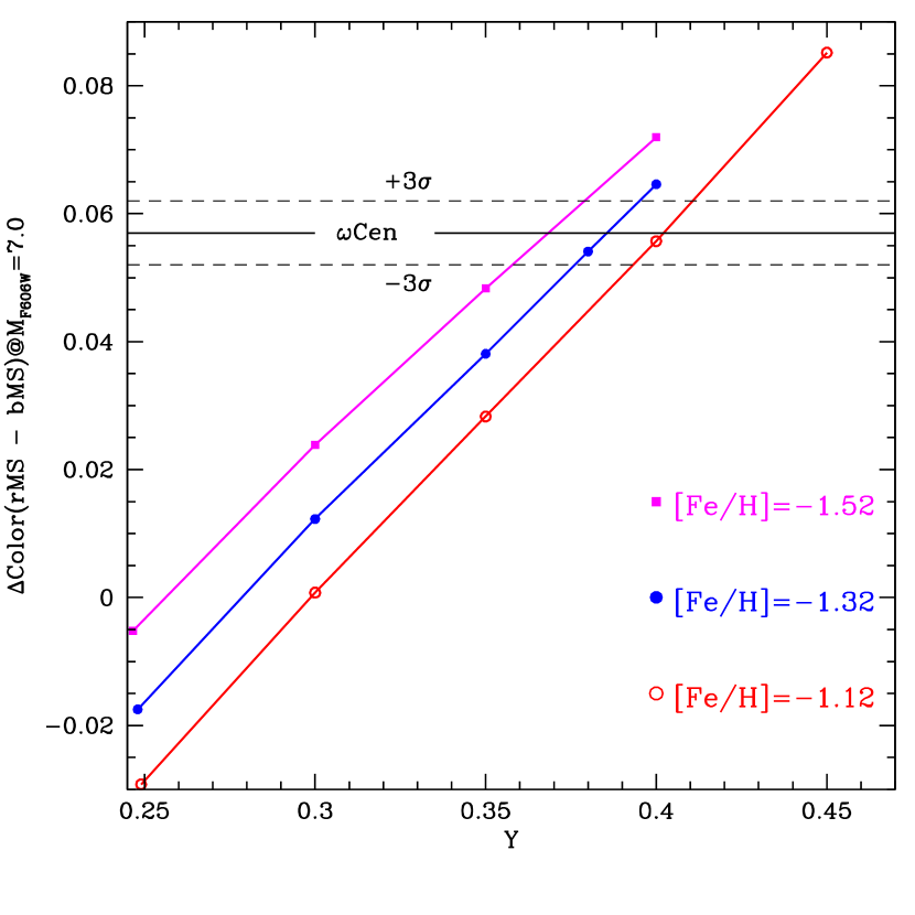
Figure 4: Theoretical estimate of the parameter $\Delta C$ as a function of the initial He content of the bMS and for various assumptions about its iron content [Fe/H]. The horizontal solid line marks our measured value of $\Delta C$. The horizontal dashed lines represent the 3$\sigma$ uncertainty of that measurement.

We used our theoretical models for a comparison with the observed $\Delta C$ between the two branches of the main sequence. To do this we derived the equivalent theoretical quantity from our set of isochrones, and transformed it into the observational plane, as just indicated.

The next step was to choose metallicity values for the rMS and for the bMS, within the broad range of metal abundances that has been found in spectroscopic studies — a choice that is hampered, however, by the lack of knowledge of how the two MS branches connect to the upper parts of the HR diagram, from which all of our good abundance information comes. Thus all that we really have to go on is the uncertain result of P05 that the metallicities of the rMS and the bMS are about $-$1.6 and $-$1.3 respectively, with a somewhat less uncertain result that the difference of the two metallicities is $0.3\pm 0.2$. (They italicize the difference, marking it as their prime result concerning metallicity.)

We accordingly chose for the rMS our [Fe/H] = $-$1.62 isochrone, with primeval He (i.e., $Y=0.246$), and for the bMS the isochrones with [Fe/H] = $-$1.32 and various He abundances. In doing so, we note that it is the difference of the metallicities that matters, rather than the absolute value of either of them. We could shift these [Fe/H] values by 0.1–0.2 dex or so, without any appreciable effect on the helium abundance that we will derive for the bMS, or its uncertainty. (We have, in fact, verified that our results remain the same if we choose [Fe/H] = $-$1.75 for the rMS and also shift all the bMS [Fe/H] values by the same 0.13.)

For comparison with observation, then, we calculated the color difference at $M_{\rm F606W}=7.0$ between the rMS isochrone and the bMS isochrones, with various assumed values of the helium abundance $Y$. Bearing in mind, however, that P05 considered the metallicity difference between the bMS and rMS to be uncertain by 0.2, we also carried out the same procedure for assumed bMS metallicities of $-$1.12 or $-$1.52 (i.e., higher or lower by 0.2).

Figure 4 shows these theoretical $\Delta C$ estimates. In order to make our procedures clear, we explain at length the meanings of the various lines in the figure: Each of the three sloping lines corresponds to the bMS metallicity that is indicated for that line in the color key. Each point on the line shows the value of $\Delta C$ that comes from assuming that value of metallicity for the bMS, along with a particular value of $Y$, while always using for the rMS [Fe/H] = $-$1.62 and $Y=0.246$. The lines themselves were created by connecting with straight lines the points belonging to the same bMS metallicity.

We used the figure to determine the value of the helium abundance $Y$, and also its uncertainty. The latter arises from two sources: the uncertainty in the metallicity difference between the bMS and the rMS, and our observational error in measuring $\Delta C$.

The solid horizontal line in the figure corresponds to our measured value of $\Delta C$. It serves two purposes: First, its intersection with the sloping line for [Fe/H] = $-$1.32 (our preferred value for the bMS) is at $Y$ = 0.0386; this is our result for the helium abundance. Second, this line also tells us the uncertainty in $Y$ that results from the uncertainty of 0.2 in the metallicity of the bMS relative to the rMS. To evaluate that uncertainty we simply measure the distance from the intersection of the solid horizontal line with the [Fe/H] = $-$1.32 line to its intersection point with either the [Fe/H] = $-$1.12 or the $-$1.52 line. These distances are each 0.016, which is thus the uncertainty in $Y$ due to this cause.

The second source of uncertainty in $Y$ comes from the measuring error in $\Delta C$. To represent this, we drew the two horizontal dashed lines, which are above and below the solid line by the $3\sigma=\pm 0.005$ that we chose as a conservative error estimate. They intersect the sloping [Fe/H] = $-$1.32 line at $Y$ = 0.375 and 0.397 respectively, 0.011 greater or less than our $Y$ value of 0.386.

When we combine this $\pm$0.011 with the $\pm$0.016 that came from the uncertainty in the metallicity difference, our result for the helium abundance of the bMS is $Y=0.39\pm 0.02$. Not only is this a more reliable estimate than has been available before; it is the first estimate that has had a quantitative uncertainty attached.

Recently, Pasquini et al. (2011) have used the He $\lambda$10830 line in the spectra of two red-giant stars in NGC 2808 to estimate that the He abundance of those stars is $Y\geq 0.39$. It is interesting to see the similarity with what we find in $\omega$ Cen. Additionally, in $\omega$ Cen itself Dupree, Strader, & Smith (2011) have detected the $\lambda$10830 line in some RGB stars but not in others, in agreement with our suggestion that some of the cluster stars have enhanced helium.

3.2 The isochrones

Figure 5 shows the isochrones that correspond to the abundances with which we have fitted the color separation between the bMS and the rMS (along with a third isochrone that will be discussed in Section 5). An isochrone with primeval helium and a metallicity appropriate for $\omega$ Cen fits the rMS, while, as just explained, we fit the bMS with an [Fe/H] that is higher by $\sim$0.3, and helium content $Y=0.386$. We find it gratifying that the theoretical isochrones fit the bMS and the rMS as well as they do, especially since the fitting is a direct overplot, with no adjustments other than our having chosen the abundances so as to match the observed colors at $m_{\rm F606W}=21.1$.

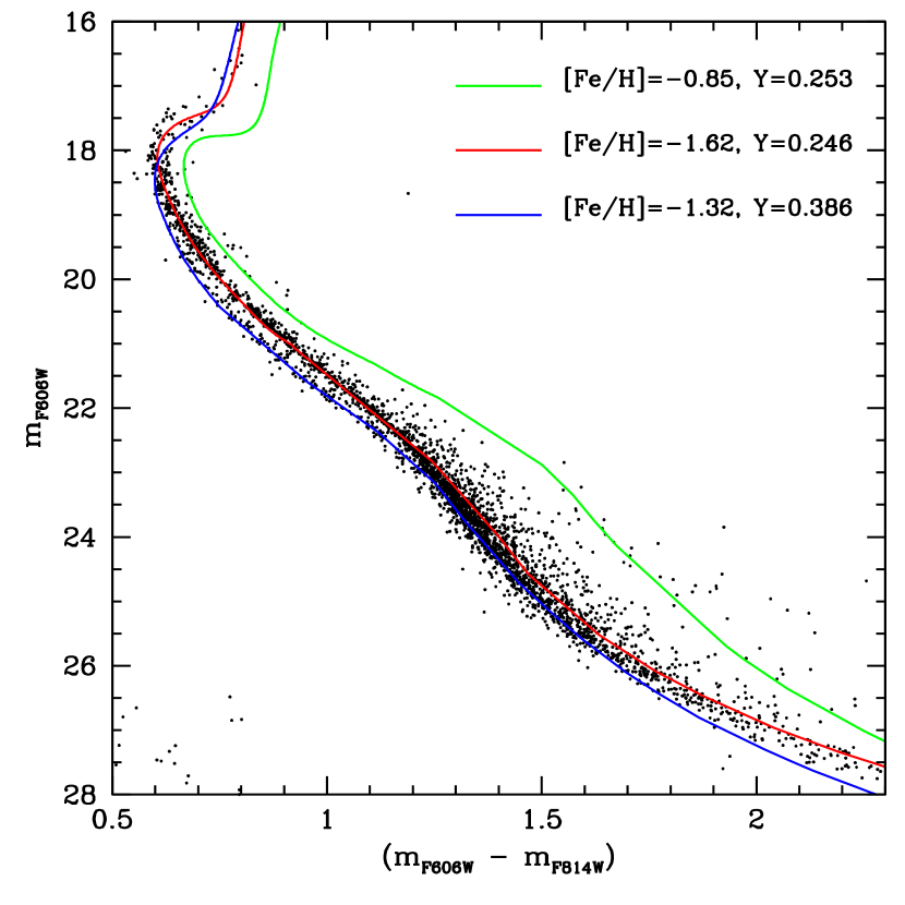
Figure 5: Comparison of selected theoretical isochrones with the CMD of the outer field. The isochrones drawn in red and in blue were chosen by merely matching the colors of the bMS and the rMS at $m_{\rm F606W}=21.17$. The isochrone in green will be discussed in Section 5.

4 A New Color-Magnitude Diagram for the Central Field

Our CMD of the outer field is photometrically accurate, and free of field stars, but it has too few stars for us to draw clear conclusions from it alone. To illuminate what the outer field is telling us, we will compare its CMD with that of the much richer central field, as measured through the same pair of filters. For this purpose, we improve on the results of the HST Treasury Survey of globular clusters (Sarajedini et al. 2007, Anderson et al. 2008), in two ways: first we follow the suggestions of Anderson et al. (2008, Sect. 7.1) regarding the use of quality indices to select a sample of the best-measured stars, and then we correct the Treasury photometry of the selected stars for differential reddening. We do not make a proper-motion selection, however, because the central field is so rich that only a tiny fraction of the total number of stars are field stars, and restricting our attention to a proper-motion sample would have caused us to lose all the faint stars.

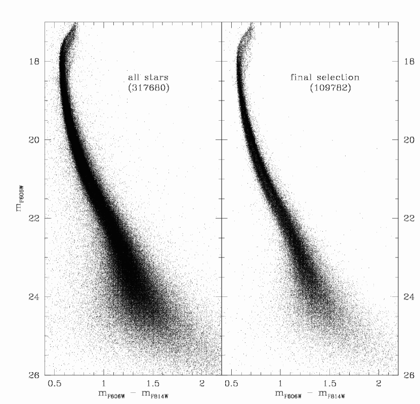
Figure 6: Comparison of a portion of the CMD of the central field, before and after selection of the stars that are the most likely to be photometrically reliable.

4.1 Photometric Quality Selection

Our photometric quality criteria were four in number: The first two were the rms residuals of the magnitude measures in each band (columns headed “err” in the Globular Cluster Treasury files at http://www.astro.ufl.edu/$\sim$ata/public_hstgc/), while the other two were xsig and ysig, which are not internal errors but rather the differences between the mean positions measured in F606W and in F814W, for the $x$ and $y$ coordinates respectively. (Experience in working with the Treasury results had shown that stars with low-quality photometry tended also to have larger values of xsig and ysig.) We plotted each criterion against magnitude, and then tried rejecting stars at various percentile levels of the criteria. We found that a good compromise between improving the CMD, on the one hand, and rejecting too many stars on the other hand, was to reject stars that were above the 75th percentile of any of the four criteria. This process, illustrated in Figure 6, selected 109,782 of the 317,680 stars that had at least two deep exposures in each filter. The cut is severe, but that is understandable in a field as crowded as the center of $\omega$ Centauri, and we believe that the resulting CMD is as good as we can produce for this field by quality selection alone.

(As a test of the efficacy of the individual criteria we verified that each of them rejected numerous stars that had passed all the other criteria at the 75th percentile level. We note that we also tried four additional criteria, which measure the quality of the PSF fit and the amount of encroaching light from neighboring stars, for each filter — called qv, qi, ov, and oi by Anderson et al. 2008. We found that these criteria rejected few stars that were not already flagged by the four that we did use; we concluded that such low levels of rejection could be attributed to random scatter of the values of those criteria, and we therefore did not use them at all.)

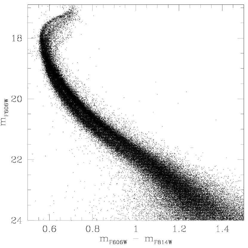
Figure 7: The CMD of the central field, after quality selection and reddening correction.

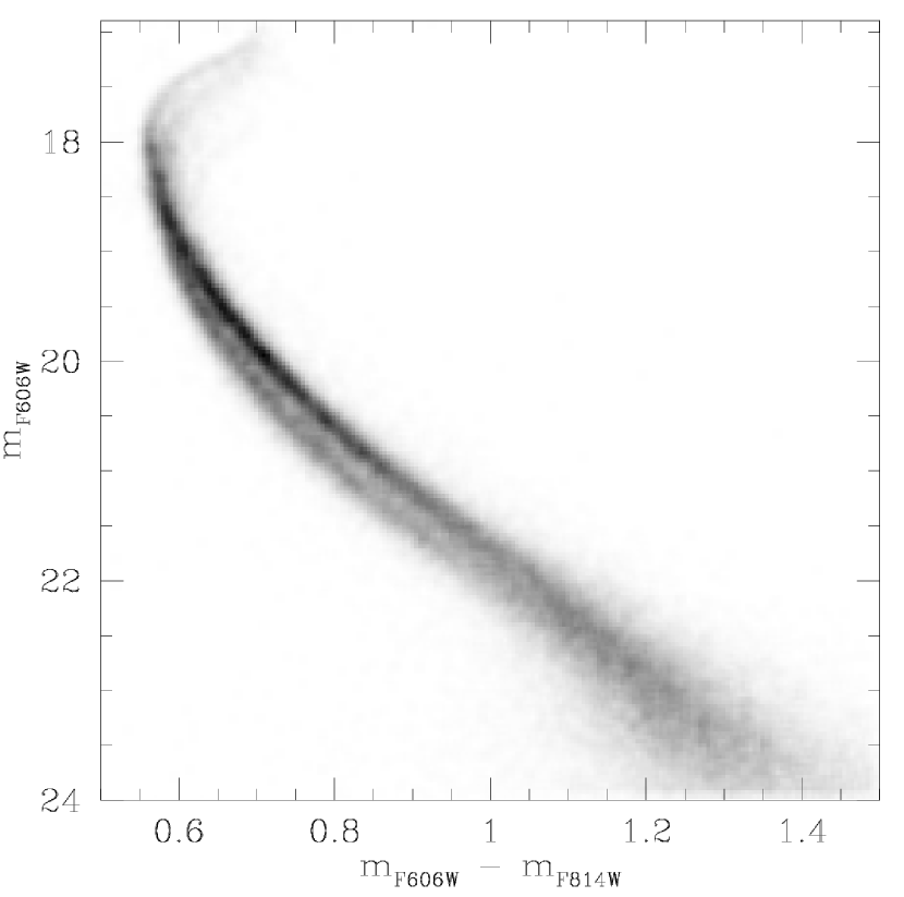
Figure 8: The CMD of the central field, after quality selection and reddening correction, shown as a Hess diagram. This gray-scale representation was made from the same colors and magnitudes that were shown in Fig. 7.

4.2 Corrections for Differential Reddening

The sequences in the CMD of $\omega$ Cen are somewhat broadened by differential reddening. The Harris (2010) catalog gives for this cluster $E(B-V)=0.12$, and reddening as large as this is rarely uniform. The basic method that we used to construct a reddening map of our field depends on drawing a fiducial sequence to follow the course of the MS, SGB, and RGB, and then deriving an approximate reddening from the observed color of each star, by seeing how far it needs to be slid up or down a reddening line in order to meet the fiducial sequence. Our usual procedure would then be to designate the well-observed stars in a bright interval of magnitude as reference stars, and to take for the reddening correction of each individual star the mean reddening of the 75 nearest reference stars. For $\omega$ Cen, however, there are special problems, because the multiplicity of sequences confuses the procedure. In this case we proceeded as follows:

We began, as we have for other clusters, by rotating the CMD through an angle

$$\theta=\tan^{-1}{A_{\rm F606W}\over A_{\rm F606W}-A_{\rm F814W}}\,,$$

around an arbitrarily chosen point. This rotation makes the reddening line into the new $x$ axis, greatly simplifying the de-reddening operation, which is now just a shift along the $x$ axis.

For the special problem of $\omega$ Cen, we iterated the first part of our usual procedure. As a first approximation to a fiducial sequence, we arbitrarily drew a line along the rMS, simply because it is the more populous of the MS components. We then applied our usual procedure, even though it is imperfect because of the multiple sequences; it did produce enough differential-reddening correction to effect some narrowing of the MS. (Because the rMS is so dominant numerically, any attempt to move bMS stars onto the rMS merely introduces noise that slows the convergence.) Four iterations of the correction procedure sufficed to give as good a correction as we could get.

In the corrected CMD (Fig. 7) the subgiant region is split into multiple branches (a foretaste of what we may hope to find with a richer set of filters). The MS split has become less prominent here, but only as a result of printing the CMD heavily enough to show the details of the subgiant region. Fig. 8 is a Hess diagram made from the same colors and magnitudes. The split in the main sequence can be seen more clearly now — strikingly well, in fact, for the crowded center of the cluster.

5 Superposition of the Two Color-Magnitude Diagrams

We now have a CMD of the outer field, quite sharp and almost completely free of field stars, but with few stars overall; and we have a CMD of the central field in the same two filters, with a much larger number of stars but with photometry of lower quality, in that crowded region. A fruitful step now is to compare the two CMDs by laying one on top of the other. In order to make this superposition, however, we need to adjust the zero points of the reddening-corrected magnitudes, because the corrections did not preserve zero points. We did this adjustment by eye, simply by getting the best match that we could.

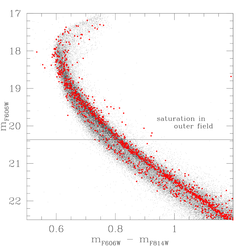
Figure 9: The points from the outer field, in red, superposed on points from the central field, in black. This figure shows the bright part of the magnitude range covered by our observations, while Fig. 10 shows the faint part of the range (with considerable magnitude overlap between the two).

The superposition, which now allows us to combine the clarity and purity of the outer field with the richness and continuity of the sequences that we see in the central field, is shown in Figures 9 and 10. The first of them shows the bright part of the magnitude range, and the second shows the faint part (with considerable magnitude overlap between the two).

In Fig. 9, the rMS appears to continue upward into the bright edge of the subgiant-branch (SGB) stars, while the bMS seems to emerge from the crossing of the bMS and rMS at a magnitude level that takes it into the next-most-prominent of the SGB sequences. Although a result that depends on photometry of saturated star images must always be taken with some reserve, it is hard to see how any other connection of branches of the MS with branches in the SGB region could be possible, given the numbers of stars along each of the two sequences, on the MS and then in the SGB region. (It is interesting to note that the detailed study of Villanova et al. 2007, which was limited to ground-based resolution beyond the central $10^{\prime}\times 10^{\prime}$ of the cluster, made SGB connections for the rMS and for the reddest branch of the MS [which they called MS-a], but they were unable to make a connection for the bMS. It is our superposition of the CMD of the outer field on that of the central field that has allowed us to suggest a SGB connection for the bMS.)

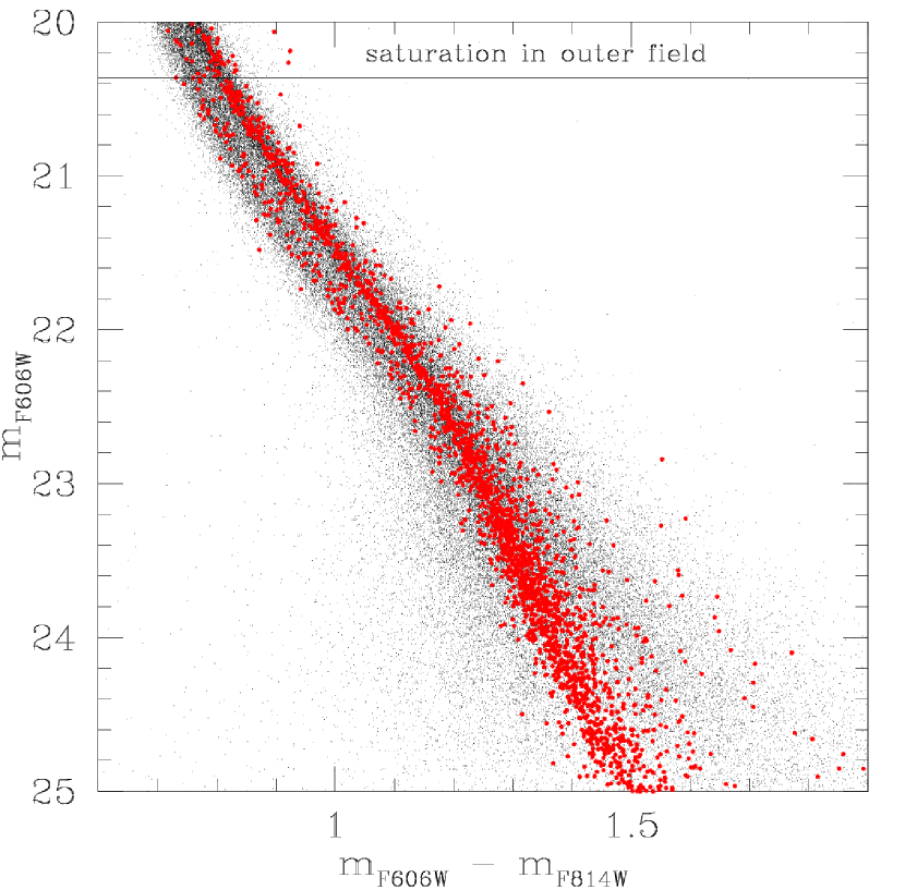
Figure 10: The faint end of the superposition of the CMD of the outer field (red) on that of the central field (black).

In Figure 10 we show the fainter part of the superposed CMDs. Here the bMS seems to intersect the rMS at magnitude $\sim 22.8$, but it is not at all clear whether this is a crossing or a merger. There is a faint hint that the bMS might emerge on the red side of the rMS at fainter magnitudes, but it is impossible to be sure of this, because the photometry in the central field rapidly loses accuracy, and below $m_{\rm F606W}\sim 23$ photometric error begins to spread the MS hopelessly.

We have already called attention to the group of faint red stars well to the red of the MS, in the outer field; we see now that they are prominent in the central field too. Although we have given up hope of tracing sequences at such faint magnitudes, what we can say nevertheless is that the magnitude spread is clearly greater on the red side of the MS than on the blue side, so that this redward extension must be something real.

We have noted that the faint red stars cannot be explained away as binaries, since they were shown in Fig. 3 to be well above the upper limit of the region in the CMD where binaries lie. Since a redder MS color is usually associated with a higher metallicity (with the notable exception of the bMS!), these stars might be suspected to be the lower end of the faintest SGB sequence (the region that Villanova et al. 2007 called MS-a). This component of $\omega$ Cen is known to be much less metal-poor, with [Fe/H] $-$0.8 to $-$0.7 (Johnson & Pilachowski 2010). In Fig. 5 we have chosen from our library of isochrones the one with [Fe/H] = $-$0.85, $Y=0.253$, and age 13 Gyr. (Noting that the highly enhanced helium in the bMS and in a few stars in NGC 2808 is an unusual anomaly, we chose to revert to a more normal $Y$, raising its value just a little as a consequence of the increased metallicity, and using a conventional value of $dY/dZ$.)

On the other hand, the spread of the red stars in color is far greater than can be expected in any single sequence, nor can we confidently trace in the observed CMD a sequence that connects SGB-a with these stars — and in fact in Villanova et al. (2007) we suggested tentatively that MS-a continues down into the rMS at a brighter magnitude than this. It is unfortunate that the outer field does not have enough stars to allow the tracing of any but the two richest sequences, while at faint magnitudes the photometry of the central field is too damaged by crowding to yield further enlightenment.

With observations that are confined to these two filters, we can go no farther in tracing sequences. It has recently been shown by Bellini et al. (2010), however, that when observations with the ultraviolet filters of WFC3 are brought into the picture, all sorts of details emerge. We will therefore leave further pursuit of the continuity of sequences to future papers that include results from more filters.

6 Summary

We have used HST ACS/WFC imaging of an outer field of $\omega$ Centauri at two epochs to derive a color-magnitude diagram, cleaned of field stars, that shows the clearest separation of the blue and red branches of the main sequence that has yet been achieved. We have calculated new stellar-structure models for a mesh of abundances of helium and metals, and have fitted isochrones to our observed sequences, deducing for the blue branch of the main sequence $Y=0.39\pm 0.02$ — the first time that this anomalous abundance of helium has been given a solid base in theory, and assigned a quantitative uncertainty. We show a plausible fit of the $\omega$ Cen sequences with three different isochrones that have different abundances of helium and metals.

We have re-examined the CMD of the central part of $\omega$ Cen, selected a subset of stars that are likely to have the most reliable photometry, and corrected its photometry for differential reddening. When we superpose the CMDs of the two regions, we tentatively identify the SGB continuation of the bMS with one of the many branches that the rich central field shows in the SGB region. We also find a striking new group of stars to the red of the main sequence. We look forward to new insights from combining these results with the leverage that UV photometry with WFC3 now applies to this extraordinarily complex CMD.

Allard F., Hauschildt, P. H., Alexander, D. R., & Starrfield, S.M., 1997, ARA&A, 35, 137

Anderson, J. 1997, Ph.D. thesis, Univ. of Calif., Berkeley

Anderson, J. 2002, in Proceedings of the 2002 HST Calibration Workshop, ed. S. Arribas, A. Koekemoer, & B. Whitmore (Baltimore: STScI), p. 13

Anderson, J. 2006, in Proceedings of the 2005 Calibration Workshop, ed. A. Koekemoer, P. Goudfrooij, & L. Dressel (Baltimore: STScI), p. 11

Anderson, J., & King, I. R. 2006, ACS Instrument Science Report 2006-01

Anderson, J., et al. 2008, AJ, 135, 2055

Bedin, L. R., Piotto, G., Anderson, J., Cassisi, S., King, I. R., Momany, Y., & Carraro, G. 2004, ApJ, 605, L125

Bedin, L. R., 2005, Cassisi, S., Castelli, F., Piotto, G., Anderson, J., Salaris, M., Momany, Y., & Pietrinferni, A. MNRAS, 357, 1038

Bellini, A., Piotto, G., Bedin, L. R., King, I. R., Anderson, J., Milone, A. P., & Momany, Y. 2009, A&A, 507, 1393

Bellini, A., Bedin, L. R., Piotto, G., Milone, A. P., Marino, A. F., & Villanova, S. 2010, AJ, 140, 631

Bragaglia, A., Carretta, E., Gratton, R., D’Orazi, V., Cassisi, S., & Lucatello, S. 2010a, A&A, 519, A60

Bragaglia, A., Carretta, E., Gratton, R. G., Lucatello, S., Milone, A., Piotto, G., D’Orazi, V., Cassisi, S., Sneden, C., & Bedin, L. R. 2010b, ApJ, 720, L41

Cannon, R. D., & Stobie, R. S. 1973, MNRAS, 162, 207

Cardelli, J. A., Clayton, G. C., & Mathis, J. S. 1989, ApJ, 345, 245

D’Antona, F., & Caloi, V. 2008, MNRAS, 390, 693

Del Principe, M., et al. 2006, ApJ, 652, 362

Dickens, R. J., & Woolley, R. v. d. R. 1967, R. Obs. Bull., 128, 255

Dupree, A. K., Strader, J., & Smith, G. H. 2011, ApJ, 728, 155

Ferguson, J. W., Alexander, D. R., Allard, F., Barman, T., Bodnarik, J. G., Hauschildt, P. H., Heffner-Wong, A., & Tamanai, A. 2005, ApJ, 623, 585

Freeman, K. C., & Rodgers, A. W. 1975, ApJ, 201, L71

Gilliland, R. 2004, ACS Instrument Science Report 2004-01

Gratton, R. G., Carretta, E., Bragaglia, A., Lucatello, S., & D’Orazi, V. 2010, A&A, 517, A81

Harris, W. E. 2010, arXiv 1012.3224

Hauschildt, P. H., Allard, F., & Baron, E. 1999a, ApJ, 512, 377

Hauschildt, P. H., Allard, F., Ferguson, J., Baron E., & Alexander, D. 1999b, ApJ, 525, 871

Johnson, C. I., & Pilachowski, C. A. 2010, ApJ. 722, 1373

Lee, Y.-W., Joo, J.-M., Sohn, Y.-J., Rey, S.-C., Lee, H.-C., & Walker, A. R. 1999, Nature, 402, 55

Merritt, D., Meylan, G., & Mayor, M. 1997, AJ, 114, 1074

Norris, J. 2004, ApJ, 612, L25

Norris, J. E., Freeman, K. C., & Mighell, K. J. 1996, ApJ, 462, 241

Pancino, E., Ferraro, F., Bellazzini, M., Piotto, G., & Zoccali, M. 2000, ApJ, 534, 83

Pasquini, L., Mauas, P., Käufl, H. U.,& Cacciari, C. 2011, A&A, 531, A35

Pietrinferni, A., Cassisi, S., Salaris, M., & Castelli, F. 2004, ApJ, 612, 168

Pietrinferni, A., Cassisi, S., Salaris, M., & Castelli, F. 2006, ApJ, 642, 797

Piotto, G., et al. 2005, ApJ, 621, 777

Piotto, G., et al. 2007, ApJ, 661, L53

Rogers, F. J., & Iglesias, C. A. 1992, ApJS, 79, 507

Sarajedini, A., et al. 2007, AJ, 133, 1658

Saumon, D., Chabrier, G., & van Horn, H. M. 1995, ApJS, 99, 713

Sirianni, M., et al. 2005, PASP, 117, 1049

Sollima, A., Pancino, E., Ferraro, F. R., Bellazzini, M., Straniero, O., & Pasquini, L. 2005, ApJ, 634, 332

Villanova, S., et al. 2007, ApJ, 663, 296