Turbulent dynamos with advective magnetic helicity flux

Abstract

Many astrophysical bodies harbor magnetic fields that are thought to be sustained by a dynamo process. However, it has been argued that the production of large-scale magnetic fields by mean-field dynamo action is strongly suppressed at large magnetic Reynolds numbers owing to the conservation of magnetic helicity. This phenomenon is known as catastrophic quenching. Advection of magnetic fields by stellar and galactic winds toward the outer boundaries and away from the dynamo is expected to alleviate such quenching. Here we explore the relative roles played by advective and turbulent–diffusive fluxes of magnetic helicity in the dynamo. In particular, we study how the dynamo is affected by advection. We do this by performing direct numerical simulations of a turbulent dynamo of $\alpha^{2}$ type driven by forced turbulence in a Cartesian domain in the presence of a flow away from the equator where helicity changes sign. Our results indicate that in the presence of advection, the dynamo, otherwise stationary, becomes oscillatory. We confirm an earlier result for turbulent–diffusive magnetic helicity fluxes that for small magnetic Reynolds numbers (${{\rm Rm}}\lesssim 100...200$, based on the wavenumber of the energy-carrying eddies) the magnetic helicity flux scales less strongly with magnetic Reynolds number (${{\rm Rm}}^{-1/2}$) than the term describing magnetic helicity destruction by resistivity (${{\rm Rm}}^{-1}$). Our new results now suggest that for larger ${{\rm Rm}}$ the former becomes approximately independent of ${{\rm Rm}}$, while the latter falls off more slowly. We show for the first time that both for weak and stronger winds, the magnetic helicity flux term becomes comparable to the resistive term for ${{\rm Rm}}\gtrsim 1000$, which is necessary for alleviating catastrophic quenching.

1 Introduction

A theoretical framework for explaining the large-scale magnetic fields observed in many astrophysical bodies is mean-field dynamo theory. Its basic idea is that the inductive effects of turbulent motions are able to amplify a weak magnetic field and maintain it on timescales longer than the magnetic diffusion time (Moffatt, 1978). Gradients in the large-scale velocity field, like shear motions, can also contribute significantly to the amplification of the magnetic field. In mean-field dynamo theory the contribution of the turbulent scales is parameterized through the electromotive force which depends on the large-scale magnetic field as well as its derivatives (Krause & Rädler, 1980). The coefficients in front of the magnetic field and its derivatives are called turbulent transport coefficients. They can describe either turbulent–diffusive (with turbulent diffusion $\propto\eta_{\rm t}$) or non-diffusive (e.g., the $\alpha$ effect or turbulent pumping) effects.

Under some approximations (e.g., in the low conductivity limit for small magnetic Reynolds number, ${{\rm Rm}}\leq 1$, or in the high conductivity limit for short correlation times, i.e., small Strouhal number, ${\rm St}\leq 1$), theories like the first order smoothing approximation are able to predict the functional form of the expressions and the correct values of the coefficients. Within their limits of validity, these results present a remarkably good agreement with the computation of the transport coefficients through direct numerical simulations (DNS); see, e.g., Sur et al. (2008). However, not enough is known about the functional form of these coefficients at large values of ${{\rm Rm}}$ (i.e., small values of the microphysical magnetic diffusivity) and about the saturation process when the magnetic field becomes dynamically important. Understanding the behavior of the dynamo in these regimes has remained an important problem for several decades. Although many recent works have contributed to understanding dynamo saturation at large magnetic Reynolds numbers, more work is still necessary to have a complete picture of the dynamo excitation and saturation mechanisms.

Among the turbulent transport coefficients the $\alpha$ effect is particularly important, because it allows a closed dynamo loop for regenerating both poloidal and toroidal magnetic fields. It has been suspected, however, that in closed or triply periodic domains the $\alpha$ effect can be strongly suppressed at higher magnetic Reynolds numbers and might scale like $\alpha\propto{{\rm Rm}}^{-1}$ (Vainshtein & Cattaneo, 1992; Cattaneo & Hughes, 1996). An explanation for this was proposed by Gruzinov & Diamond (1994), who used the $\alpha$ effect derived by Pouquet et al. (1976), which has, in addition to the kinetic helicity density, a contribution proportional to the current helicity density. It is this quantity which builds up as the dynamo saturates.

This is a consequence of magnetic helicity conservation and can be explained as follows: the large-scale magnetic field generated by the $\alpha$ effect is helical, but in order to satisfy the conservation of total magnetic helicity, a small-scale field with equally strong magnetic helicity of opposite sign must be generated in the system. The small-scale magnetic helicity is responsible for the creation of a magnetic $\alpha$ effect ($\alpha_{\rm M}$) which contributes with opposite sign to the kinetic $\alpha$. This basic idea led Kleeorin & Ruzmaikin (1982) to propose the dynamical quenching model at a time well before simulations saw any indications of catastrophic quenching. Even nowadays the issue is quite unclear when it comes to making predictions about the high-${{\rm Rm}}$ regime. The final amplitude that the magnetic $\alpha$ effect acquired depends on the geometry of the system and on the value of the magnetic Reynolds number. For highly turbulent astrophysical objects with high ${{\rm Rm}}$ like the Sun or the Galaxy, $\alpha_{\rm M}$ could attain higher amplitudes, decreasing then the dynamo efficiency. However, the dynamics of $\alpha_{\rm M}$ also depends on the ability of the system to get rid of the small-scale magnetic helicity responsible for its creation. In a closed or triply periodic homogeneous domain, magnetic helicity annihilation depends just on the microscopic magnetic diffusivity. This is a very slow process given the scales and diffusivity values under consideration. However, an obvious solution to this catastrophic (${{\rm Rm}}$-dependent) quenching is to allow the system to get rid of helical small-scale magnetic fields.

In real astrophysical systems, this processes is generally expected to happen in a number of different ways. Among the various mechanisms for removing magnetic helicity from the system we focus here on the role played by the turbulent–diffusive magnetic helicity flux and by the presence of advective flows or winds. The role of these magnetic helicity fluxes has been tested in the context of mean-field dynamo models through a dynamical equation for the magnetic $\alpha$-effect (Kleeorin et al., 2000; Brandenburg & Subramanian, 2005; Shukurov et al., 2006; Sur et al., 2007; Brandenburg et al., 2009; Guerrero et al., 2010; Chatterjee et al., 2011). These models have demonstrated the importance of magnetic helicity fluxes in solving the catastrophic quenching problem.

Verifying the validity of these results in DNS is more complicated since obtaining higher ${{\rm Rm}}$ in the numerical models requires high resolution and large computational resources. Various attempts have, however, succeeded in demonstrating the role of magnetic helicity conservation in the saturation of the dynamo. For instance, Brandenburg (2001) studied the saturation in triply periodic helically forced dynamos of $\alpha^{2}$ type. The role of open magnetic boundary conditions for convective dynamos has been studied in Käpylä et al. (2008, 2009, 2010). Furthermore, using forced turbulence, Mitra et al. (2010a) (hereafter MCCTB) have verified the existence of turbulent–diffusive magnetic helicity fluxes in $\alpha^{2}$ dynamo models in the presence of an equator and Hubbard & Brandenburg (2010) (hereafter HB) did the same for a dynamo region embedded inside a highly conducting halo which provided a more realistic boundary condition. In both cases it was found that a fit to a Fickian diffusion law can account for this flux and that the diffusivity value is comparable to or below the value of the turbulent magnetic diffusivity $\eta_{\rm t}$. The resulting Fickian diffusion coefficient was found to be approximately independent of ${{\rm Rm}}$. By considering a statistically steady state, and noting that the local value of the magnetic helicity density was also statistically steady, their result became then also independent of the gauge chosen to define the magnetic vector potential.

In addition, shear flows have been argued to be effective in alleviating catastrophic quenching (Vishniac & Cho, 2001) and allowing significant saturation levels of the dynamo (Käpylä et al., 2008), although it appears now plausible that their result could also be explained through a change in the excitation conditions of the dynamo. Indeed, recent DNS have failed to demonstrate the presence of the Vishniac-Cho flux (Hubbard & Brandenburg, 2011). Yet another possibility is the advective magnetic helicity flux. In the context of the galactic dynamo, alleviation of catastrophic quenching thanks to a wind has been studied in mean-field models by Shukurov et al. (2006) and Sur et al. (2007). Mitra et al. (2011) studied the role of a wind in solar mean-field dynamo models. The models studied in the present paper allow us to compare with their results and to determine the importance of magnetic helicity fluxes in the dynamical evolution of the magnetic $\alpha$-effect. To our understanding the study of advective fluxes in DNS of a dynamo is an outstanding problem. With this paper we intend to close this gap.

We perform DNS leading to $\alpha^{2}$-type dynamo action in a domain with kinetic helicity of opposite signs on both sides of the equator. We use a relaxation term to include a large-scale flow that advects the large-scale magnetic field. Furthermore, we consider periodic boundary conditions in the horizontal directions, zero-gradient conditions for the velocity and vertical field conditions for the magnetic field. In this way we allow for the removal of magnetic helicity through advection. For the sake of simplicity and to study these effects separately in a clear way, we do not include large-scale shear. Nevertheless the results presented here should also be applicable in the context of the galactic dynamo and, in principle, also to the solar dynamo, where large-scale winds have been shown in mean-field models to play a role in carrying magnetic helicity outside its bounds (Mitra et al., 2011).

This paper is organized as follows. In Sect. 2 we describe the physical model considered here and present the equations governing its evolution. In Sect. 3 we present the results of the simulations. First we describe the properties of the solutions without the wind. Next, we explore the effects that the wind has on the characteristics of the dynamo solution. Finally, we determine the magnetic helicity fluxes present in the model and verify their balance with the production terms to prevent the quenching of what corresponds to the $\alpha$ effect in the related mean-field description. We conclude and summarize the results in Sect. 4.

2 The model

2.1 Governing equations

We use the Pencil Code to solve the following set of compressible hydromagnetic equations in an isothermal layer:

$$\frac{\partial\bm{A}}{\partial t}=\bm{U}\times\bm{B}-\mu_{0}\eta{\bm{J}},$$ (1)

$$\frac{{\rm{D}}\bm{U}}{{\rm{D}}t}=-c_{\rm s}^{2}\mbox{\boldmath$\nabla$}{}\ln\rho+\frac{1}{\rho}\bm{J}\times{\bm{B}}+\frac{1}{\rho}\bm{\nabla}\cdot 2\nu\rho\mbox{\boldmath${\sf S}$}+\bm{f}_{\rm w}+\bm{f},$$ (2)

$$\frac{{\rm{D}}\ln\rho}{{\rm{D}}t}=-\mbox{\boldmath$\nabla$}{}\cdot{\bm{U}}+q_{\rho},$$ (3)

where ${\rm{D}}/{\rm{D}}t=\partial/\partial t+\bm{U}\cdot\bm{\nabla}$ is the advective derivative, $\bm{A}$ is the magnetic vector potential, $\bm{B}=\bm{\nabla}\times\bm{A}$ is the magnetic field, $\bm{J}=\bm{\nabla}\times\bm{B}/\mu_{0}$ is the current density, $\mu_{0}$ is the magnetic permeability, $\eta$ and $\nu$ are magnetic diffusivity and kinematic viscosity, respectively, $c_{\rm s}=\mbox{const}$ is the sound speed, $\bm{U}$ is the velocity, $\rho$ is the density, ${\sf S}$ is the rate of strain tensor given by

$${\sf S}_{ij}={\textstyle{1\over 2}}(U_{i,j}+U_{j,i})-{\textstyle{1\over 3}}\delta_{ij}\mbox{\boldmath$\nabla$}{}\cdot\bm{U},$$ (4)

where the commas denote derivatives, $\bm{f}_{\rm w}$ provides a forcing for the wind (defined below in Section 2.2), $q_{\rho}$ is a source term in Eq. (3) needed to replenish the resulting mass loss, $\bm{f}$ is a time-dependent random $\delta$-correlated forcing function of the form

$$\bm{f}=\bm{f}(\bm{x},t;\sigma(z)),$$ (5)

where $\sigma$ is related to its local helicity density,

$$\langle\bm{f}\cdot\mbox{\boldmath$\nabla$}{}\times\bm{f}\rangle/\langle k_{\rm f}\bm{f}^{2}\rangle=2\sigma/(1+\sigma^{2}),$$ (6)

and is chosen to vary like $\sigma(z)=\sin(2\pi z/L_{z})$ with a sign change across the equator at $z=0$. This forcing drives turbulence in a band of wavenumbers around $k_{\rm f}$. The modulation $\sigma(z)$ of this forcing is similar to that used by Warnecke et al. (2011) to simulate a sign change of helicity in forced turbulence in a spherical wedge.

We consider a computational domain of size $L_{x}\times L_{y}\times L_{z}$, with quadratic horizontal extent, $L_{x}=L_{y}$, using periodic boundary conditions and a vertical extent that is twice as big, $L_{z}=2L_{x}$, with $|z|\leq L_{z}/2$ (i.e., $-L_{z}/2\leq z\leq L_{z}/2$) and an equator at $z=0$. Our boundary conditions are

$$U_{x,z}=U_{y,z}=U_{z}-\overline{U}_{\rm w}=A_{x,z}=A_{y,z}=A_{z}=0$$ (7)

on the top and bottom boundaries at $z=\pm L_{z}/2\equiv\pm z_{\rm top}$. $\overline{U}_{\rm w}$ is the wind profile, defined below in Section 2.2. The lowest horizontal wavenumber in the domain is $k_{1}=2\pi/L_{x}$. In the following, we use $k_{1}$ as our inverse length unit, so $|k_{1}z|\leq 2\pi$. To eliminate boundary effects, we restrict most of the analysis to a diagnostic layer, $|z|\leq L_{*}$ with $k_{1}L_{*}=3$. For all our runs we choose $k_{\rm f}/k_{1}=4$, which is a compromise between it being large enough to allow a large-scale magnetic field to be generated and yet small enough to achieve sufficiently large values of ${{\rm Rm}}$.

We set $c_{\rm s}$ to unity in the code, so our dimensionless time is in units of the sound travel time, $(c_{\rm s}k_{1})^{-1}$. However, the relevant physics is not governed by compressibility effects, so it is more natural to quote time in turnover times, i.e., we quote instead the value of $tu_{\rm rms}k_{\rm f}$. In most of the cases reported below, the turbulent Mach number, $\rm Ma=u_{\rm rms}/c_{\rm s}$, is around 0.1. Likewise, in the code $\nu$ and $\eta$ are given in units of $c_{\rm s}/k_{1}$, but it is physically more meaningful to quote corresponding Reynolds numbers instead. Our resolution is increased with increasing values of ${{\rm Rm}}$, so the largest resolution used in this paper is $1024\times 1024\times 2048$ meshpoints. We return to this issue at the end of the paper.

2.2 Generating the wind

In our model, the advective term from the wind is given by the forcing function in Eq. (8),

$$\bm{f}_{\rm w}=-\frac{1}{\tau_{\rm w}}\left[\overline{\bm{U}}-\overline{\bm{U}}_{\rm w}(z)\right],$$ (8)

where $\overline{\bm{U}}$ is the horizontally averaged velocity field, and

$$\overline{\bm{U}}_{\rm w}(z)=U_{0}\frac{\bm{z}}{z_{\rm top}}$$ (9)

is the wind profile that increases linearly toward the $z$ boundaries. The wind profile can be modified by the turbulence and the magnetic field, but the original outflow profile tends to be restored on a timescale $\tau_{\rm w}$. The presence of a wind leads to mass loss across the vertical boundaries with a mass loss rate that depends on $U_{0}$.

Stellar winds are the main agents of mass loss in stars. In a galactic environment it is possible to observe galactic winds as well as galactic fountains. These mechanisms can be driven by the explosions of supernovae in the galactic disc. In this case a direct estimate of the mass loss rate is more complicated, given that it is expected to be very small. However, to have stationary conditions, we keep the mass in the domain constant using the source term $q_{\rho}$ in Eq. (3). This source term tends to be restored the density at each spatial point in the domain to its initial value $\rho_{0}$ on a timescale $\tau_{\rm s}=\tau_{\rm w}$. Thus, analogously to Eq. (8), we write $q_{\rho}=-\tau_{s}^{-1}(\ln\overline{\rho}-\ln\overline{\rho}_{0})$.

We study the dependence of our model on the dimensionless wind speed and the magnetic Reynolds number of the turbulence. These are defined as

$${\it S}_{\it W}=\frac{\mbox{\boldmath$\nabla$}{}\cdot\overline{U}_{\rm w}}{u_{\rm rms}k_{\rm f}},\quad{{\rm Rm}}=\frac{u_{\rm rms}}{\eta k_{\rm f}}.$$ (10)

In all cases, we use a magnetic Prandtl number of unity, i.e., $\nu/\eta=1$.

2.3 Magnetic helicity fluxes

In our model we expect two different kinds of magnetic helicity fluxes: those caused by the wind, i.e. advective magnetic helicity fluxes, and those due to turbulence in the presence of a mean gradient of the magnetic helicity density, i.e. turbulent–diffusive magnetic helicity fluxes. To assess their importance in the magnetic helicity budget, we now consider the magnetic helicity equation in the Weyl gauge which is used in Eq. (1), i.e.,

$${\partial\over\partial t}\overline{\bm{A}\cdot\bm{B}}=-2\eta\mu_{0}\overline{\bm{J}\cdot\bm{B}}-\mbox{\boldmath$\nabla$}{}\cdot\overline{\mbox{\boldmath${\cal F}$}}{},$$ (11)

where overbars denote averages over $x$ and $y$ and $\overline{\mbox{\boldmath${\cal F}$}}{}=\overline{\bm{E}\times\bm{A}}$ is the total magnetic helicity flux, with $\bm{E}=\eta\mu_{0}\bm{J}-\bm{U}\times\bm{B}$ being the electric field in the lab frame. This equation is evidently gauge-dependent; see for instance Candelaresi et al. (2011). In particular, since $\overline{\bm{A}\cdot\bm{B}}$ is not a physical quantity, it could drift – even in the steady state; see Fig. 2 of Brandenburg et al. (2002) for an example. However, if $\overline{\bm{A}\cdot\bm{B}}$ is constant in a particular gauge, then we have

$$\mbox{\boldmath$\nabla$}{}\cdot\overline{\mbox{\boldmath${\cal F}$}}{}=-2\eta\mu_{0}\overline{\bm{J}\cdot\bm{B}},$$ (12)

where now $\mbox{\boldmath$\nabla$}{}\cdot\overline{\mbox{\boldmath${\cal F}$}}{}$ must be gauge-independent, because $\bm{J}$ and $\bm{B}$ are gauge-invariant. This argument was invoked by MCCTB and HB to determine turbulent–diffusive contributions to the magnetic helicity flux.

In the present work, we are interested in two contributions to $\overline{h}=\overline{\bm{A}\cdot\bm{B}}$, one from the mean fields, $\overline{h}_{\rm m}=\overline{\bm{A}}\cdot\overline{\bm{B}}$, and one from the fluctuating fields, $\overline{h}_{\rm f}=\overline{\bm{a}\cdot\bm{b}}$. Their sum gives the total mean magnetic helicity density, i.e., $\overline{h}=\overline{h}_{\rm m}+\overline{h}_{\rm f}$. Note, however, that only $\overline{h}_{\rm f}$ is the component directly relevant for the study of catastrophic quenching, because it is approximately proportional to the current helicity density, $\overline{\bm{j}\cdot\bm{b}}$, which in turn determines the magnetic contribution to the $\alpha$ effect. [The approximate proportionality of magnetic and current helicities is non-trivial and will need to be re-assessed below; see also Fig. 3 of MCCTB and Table 2 of HB for earlier examples.]

The evolution equation for $\overline{h}_{\rm f}$ is

$${\partial\overline{h}_{\rm f}\over\partial t}=-2\overline{\mbox{\boldmath${\cal E}$}}{}\cdot\overline{\bm{B}}-2\eta\mu_{0}\,\overline{\bm{j}\cdot\bm{b}}-\mbox{\boldmath$\nabla$}{}\cdot\overline{\mbox{\boldmath${\cal F}$}}_{\rm f}{},$$ (13)

where, as mentioned above, we allow two contributions to the flux of magnetic helicity from the fluctuating field $\overline{\mbox{\boldmath${\cal F}$}}_{\rm f}{}$: an advective flux due to the wind, $\overline{\mbox{\boldmath${\cal F}$}}_{\rm f}{}^{\rm w}=\overline{h}_{\rm f}\overline{\bm{U}}_{\rm w}$, and a turbulent–diffusive flux due to turbulence, modelled here by a Fickian diffusion term down the gradient of $\overline{h}_{\rm f}$, i.e., $\overline{\mbox{\boldmath${\cal F}$}}_{\rm f}{}^{\rm diff}=-\kappa_{h}\mbox{\boldmath$\nabla$}{}\overline{h}_{\rm f}$. Here, $\overline{\mbox{\boldmath${\cal E}$}}{}=\overline{\bm{u}\times\bm{b}}$ is the electromotive force of the fluctuating field.

In the steady state, and if $\overline{h}_{\rm f}$ is then also constant (which is not guaranteed to be the case because $\overline{h}_{\rm f}$ is a priori gauge-dependent), we have

$$\mbox{\boldmath$\nabla$}{}\cdot\overline{\mbox{\boldmath${\cal F}$}}_{\rm f}{}=-2\overline{\mbox{\boldmath${\cal E}$}}{}\cdot\overline{\bm{B}}-2\eta\mu_{0}\,\overline{\bm{j}\cdot\bm{b}}.$$ (14)

Again, although $\mbox{\boldmath$\nabla$}{}\cdot\overline{\mbox{\boldmath${\cal F}$}}_{\rm f}{}$ is in principle gauge-dependent, it can now be determined by measuring $\overline{\mbox{\boldmath${\cal E}$}}{}\cdot\overline{\bm{B}}$ and $\overline{\bm{j}\cdot\bm{b}}$, that are manifestly gauge-independent quantities. This means that $\mbox{\boldmath$\nabla$}{}\cdot\overline{\mbox{\boldmath${\cal F}$}}_{\rm f}{}$ must be gauge-independent as well. We assume that $\overline{\mbox{\boldmath${\cal F}$}}_{\rm f}{}$ has a component only in the vertical direction. We can therefore obtain its $z$ dependence through integration via

$$\overline{\cal F}_{\rm f{z}}=\int_{0}^{z}\mbox{\boldmath$\nabla$}{}\cdot\overline{\mbox{\boldmath${\cal F}$}}_{\rm f}{}\,{\rm{d}}z^{\prime}.$$ (15)

The assumption of only a $z$ component of $\overline{\mbox{\boldmath${\cal F}$}}_{\rm f}{}$ would break down in the presence of shear, where cross-stream fluxes with finite divergence are possible; see Hubbard & Brandenburg (2011).

For the discussion of our results presented below, let us contrast our present simulations with those of MCCTB. In their case, the outer boundary condition at $z=\pm L_{z}/2$ was a perfect conductor (P.C.) one and the most easily excited mode was antisymmetric about the midplane with dynamo waves propagating toward the equator. This antisymmetry results in permitting a flux of magnetic helicity through the equatorial plane and in this sense has the same effect as the vertical field (V.F.) boundary condition. This, together with the fact that the magnetic helicity density is antisymmetric about the equator, is the reason why in their case the turbulent–diffusive flux can play a measurable role. However, because $\overline{\cal F}_{{\rm f}z}$ has vanishing vertical derivative at the equator, the $\mbox{\boldmath$\nabla$}{}\cdot\overline{\mbox{\boldmath${\cal F}$}}_{\rm f}{}$ vanishes there. This is different in the model of HB, in which the helicity is arranged to be symmetric about the midplane, which is therefore not an equator in the usual sense. Here the field is symmetric about the midplane, corresponding thus to a P.C. condition, and thus $\mbox{\boldmath$\nabla$}{}\cdot\overline{\mbox{\boldmath${\cal F}$}}_{\rm f}{}\neq 0$. The boundary conditions and their properties are summarized in Table 1 for MCCTB and HB and compared with those used in the present work.

Table 1: Comparison of boundary conditions and other properties of the simulations of MCCTB and the present work.

MCCTB HB present work boundary P.C. halo V.F. $\overline{\cal F}_{{\rm f}z}=0$ $\overline{\cal F}_{{\rm f}z}\neq 0$ $\overline{\cal F}_{{\rm f}z}\neq 0$ $\mbox{\boldmath$\nabla$}{}\cdot\overline{\mbox{\boldmath${\cal F}$}}_{\rm f}{}\neq 0$ $\mbox{\boldmath$\nabla$}{}\cdot\overline{\mbox{\boldmath${\cal F}$}}_{\rm f}{}=0$ $\mbox{\boldmath$\nabla$}{}\cdot\overline{\mbox{\boldmath${\cal F}$}}_{\rm f}{}=0$ equator/ antisymmetry symmetry symmetry midplane (like V.F.) (like P.C.) (like P.C.) $\overline{\cal F}_{{\rm f}z}\neq 0$ $\overline{\cal F}_{{\rm f}z}=0$ $\overline{\cal F}_{{\rm f}z}=0$ $\mbox{\boldmath$\nabla$}{}\cdot\overline{\mbox{\boldmath${\cal F}$}}_{\rm f}{}=0$ $\mbox{\boldmath$\nabla$}{}\cdot\overline{\mbox{\boldmath${\cal F}$}}_{\rm f}{}\neq 0$ $\mbox{\boldmath$\nabla$}{}\cdot\overline{\mbox{\boldmath${\cal F}$}}_{\rm f}{}=0$

Unlike MCCTB, in the present work the V.F. condition is applied on the outer boundaries, in which case the most easily excited mode is symmetric about the equator with dynamo waves travelling away from the midplane. This is similar to a P.C. condition at the midplane, for which the magnetic helicity flux vanishes. However, because $\overline{h}_{\rm f}$ is antisymmetric about the equator, it must have a turning point there, so its second derivative vanishes and $\mbox{\boldmath$\nabla$}{}\cdot\overline{\mbox{\boldmath${\cal F}$}}_{\rm f}{}=0$. The present model does not have shear, but the nature of the dominant mode is similar to early simulations of dynamos driven by the magneto-rotational instability (Brandenburg et al., 1995).

3 Results

3.1 Model without advective flux

We begin by describing the results for a dynamo in the absence of an advective flux (${\it S}_{\it W}=0$). The solution for this particular setup is a steady magnetic field mainly concentrated around the equator of the domain, where the magnetic helicity changes its sign. In Figure 1 we show the $B_{y}$ and $B_{z}$ components of the magnetic field in the saturated phase of a model without wind and ${{\rm Rm}}=206$ (later referred to as Model N3). Note that $B_{x}=B_{y}=0$ on the top and bottom boundaries, owing to the use of vertical-field boundary conditions. Both of them, as well as $B_{z}$, do not show any significant temporal change once $b_{\rm rms}$ has reached its saturation value. This can be observed in the top panel of Figure 2, where the vertical distribution of $\overline{B}_{y}$ is depicted as a function of time.

The fact that this model is steady in the absence of a wind is surprising, because according to linear mean-field calculations (Brandenburg et al., 2009) it should exhibit cyclic behavior with dynamo waves moving away from the midplane. This discrepancy could be related to nonlinearity or to differences resulting from the use of mean-field theory. However, for the different boundary conditions used by MCCTB, mean-field and direct numerical simulations exhibit rather similar behavior. If it is a consequence of nonlinearity, it could be related to not allowing magnetic helicity to escape the domain. Indeed, the behavior is certainly quite different from the cases with advective magnetic helicity flux (see below), and it is also different from the otherwise similar accretion disc models.

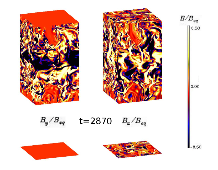
Figure 1: Visualization of $B_{y}$ (left) and $B_{z}$ (right) on the borders of the domain for model N3 in the saturated phase of the simulation ($t$ is time in turnover times).

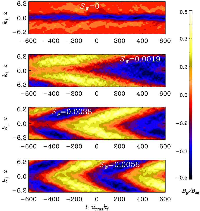
Figure 2: Space-time diagrams of $\overline{B}_{y}$ for different wind intensities ${\it S}_{\it W}$ corresponding to Models N3, W3, M2, and S2 from top to bottom. The time axes have been shifted such that for each run about 1200 turnover times are being displayed. Note that the cycle period decreases with increasing wind speed.

3.2 Model with advective flux

Figure 3: Resulting vertical profile of $\overline{U}_{z}$ together with the rms velocity as a function of height. Different lines correspond to different times. In this case $U_{0}=0.015c_{\rm s}$, corresponding to ${\it S}_{\it W}=0.0055$.

Let us now turn to models in which a wind is included (${\it S}_{\it W}\neq 0$). An example of the resulting wind profile as well as the vertical distribution of $u_{\rm rms}$ is shown in Figure 3. Even with just a weak wind the dynamo becomes oscillatory; see Figure 2. Note that the cycle period decreases as the wind speed is increased. We observe oscillatory solutions of even parity, that is $\overline{B}_{x}$ and $\overline{B}_{y}$ are on average symmetric with respect to the midplane $z=0$, with dynamo waves migrating away from $z=0$. This is expected based on mean-field models in similar setups (Brandenburg et al., 2009) provided the outer boundary condition is a vacuum or vertical field condition, as is the case here.

In Figure 4 we can see how the actual $B_{y}(x,y,z,t)$, as opposed to its horizontal average $\overline{\bm{B}}_{y}(z,t)$, evolves during half a period in the saturated phase of the simulations, changing gradually from negative to positive polarity. In Table LABEL:simulation we summarize important output parameters that characterize the simulations and, in particular, details regarding the magnetic helicity balance. Note that all table entries are non-dimensionalized by normalizing with relevant quantities such as $B_{\rm eq}$; see the table caption for details. Magnetic helicity and the various production terms are antisymmetric about the midplane. Within the range $|z|\leq L_{*}$, all these quantities vary approximately linearly with $z$. Therefore we characterize their values by their slope. An appropriate normalization is therefore $k_{1}\eta_{\rm t0}B_{\rm eq}^{2}$.

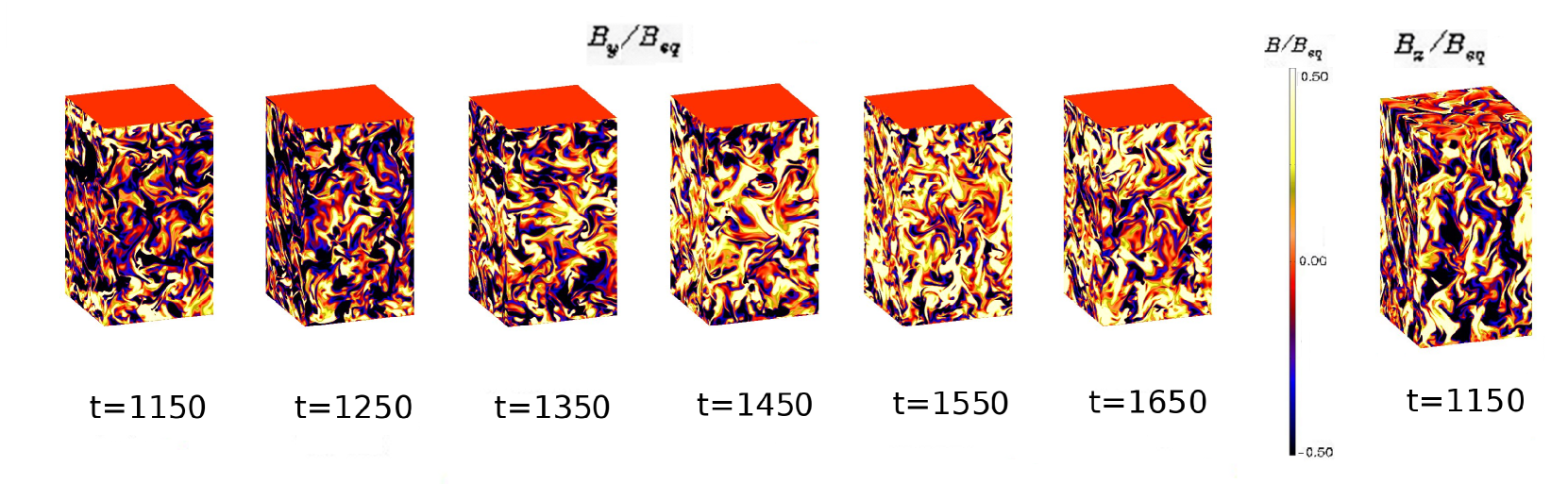
Figure 4: Visualization of $B_{y}$ (left) at six different times during the evolution of the system, for Model S3. It is visible its variability, being this component of the magnetic field prevalently negative in the first snapshot and gradually turning positive in the others. Time is given in turnover times and spans over half a cycle. On the right, $B_{z}$ is visualized on the borders of the domain for model S3. It does not show any relevant variability during its evolution.

Table 2: Characteristic output parameters of the simulations. Here, ${\it S}_{\it W}$ characterizes the wind speed, $\overline{\bm{B}}_{\rm rms}$ is the rms value of the mean field normalized by $B_{\rm eq}$, $2\overline{\mbox{\boldmath${\cal E}$}}{}\cdot\overline{\bm{B}}$, $2\eta\,\overline{\bm{j}\cdot\bm{b}}$, and $\mbox{\boldmath$\nabla$}{}\cdot\overline{\mbox{\boldmath${\cal F}$}}_{\rm f}{}$ give magnetic helicity production, dissipation, and flux divergence in units of $k_{\rm f}\eta_{\rm t0}B_{\rm eq}^{2}$, $\overline{\cal F}_{z}^{\rm diff}$ is the turbulent–diffusive magnetic helicity flux in units of $\eta_{\rm t0}B_{\rm eq}^{2}$, characterized by the diffusion coefficient $\kappa_{\rm f}/\eta_{\rm t}$, $k_{\rm eff}$ is normalized by $k_{\rm f}$, $\overline{\bm{j}\cdot\bm{b}}$ is normalized by $k_{\rm f}B_{\rm eq}^{2}$, and $\mbox{\boldmath$\nabla$}{}\cdot\overline{\mbox{\boldmath${\cal F}$}}_{\rm m}{}$ is the flux divergence of the mean field in units of $k_{\rm f}\eta_{\rm t0}B_{\rm eq}^{2}$. The strongest outflows we simulate are those of Models I1 and I2, for which we reckon that the magnetic field is manly carried out of the domain by the outflow. The outflows on which we manly focus in this work are those of Models S1 – S6, in which the maximum value of the wind speed is $U_{0}\approx 0.15\cdot u_{\rm rms}$. $N_{x}$ indicates the number of mesh points in the $x$ direction. (In all cases we have $N_{y}=N_{x}$ and $N_{z}=2N_{x}$.)

Model ${\it S}_{\it W}$ ${{\rm Rm}}$ $2\overline{\mbox{\boldmath${\cal E}$}}{}\cdot\overline{\bm{B}}$ $2\eta\,\overline{\bm{j}\cdot\bm{b}}$ $\mbox{\boldmath$\nabla$}{}\cdot\overline{\mbox{\boldmath${\cal F}$}}_{\rm f}{}$ $\overline{\cal F}_{z}^{\rm diff}$ $\kappa_{\rm f}/\eta_{\rm t}$ $k_{\rm eff}$ $\overline{\bm{j}\cdot\bm{b}}$ $\mbox{\boldmath$\nabla$}{}\cdot\overline{\mbox{\boldmath${\cal F}$}}_{\rm m}{}$ T1 0.0000 $9$ $0.066\pm 0.019$ $-0.069\pm 0.018$ $0.004\pm 0.001$ $0.007$ $-0.3\pm 0.7$ $1.22$ $-0.03$ $0.06$ T2 0.0000 $23$ $0.032\pm 0.005$ $-0.035\pm 0.003$ $0.004\pm 0.007$ $0.002$ $-0.5\pm 0.4$ $1.16$ $-0.03$ $0.03$ N1 0.0000 $37$ $0.048\pm 0.007$ $-0.047\pm 0.007$ $0.001\pm 0.001$ $0.004$ $0.1\pm 0.2$ $1.48$ $-0.07$ $0.05$ N2 0.0000 $81$ $0.023\pm 0.008$ $-0.022\pm 0.005$ $0.000\pm 0.005$ $0.002$ $-0.0\pm 0.2$ $1.37$ $-0.07$ $0.02$ N3 0.0000 $206$ $0.001\pm 0.001$ $-0.002\pm 0.000$ $0.001\pm 0.001$ $-0.003$ $0.0\pm 0.2$ $0.97\rm i$ $-0.01$ $0.00$ N4 0.0000 $397$ $0.000\pm 0.004$ $-0.001\pm 0.001$ $-0.000\pm 0.004$ $-0.000$ $0.1\pm 0.2$ $0.84\rm i$ $-0.01$ $0.00$ N5 0.0000 $722$ $-0.006\pm 0.002\ \$ $-0.005\pm 0.001$ $0.005\pm 0.005$ $0.017$ $0.1\pm 0.3$ $2.34$ $-0.16$ $-0.02\$ N6 0.0054 $1073$ $0.010\pm 0.004$ $-0.006\pm 0.000$ $-0.018\pm 0.015$ $0.019$ $0.0\pm 0.3$ $2.83$ $-0.28$ $0.02$ W1 0.0020 $24$ $0.205\pm 0.007$ $-0.196\pm 0.007$ $-0.008\pm 0.002$ $0.013$ $0.4\pm 0.1$ $1.17$ $-0.19$ $0.19$ W2 0.0019 $51$ $0.094\pm 0.022$ $-0.088\pm 0.023$ $-0.005\pm 0.001$ $0.011$ $0.5\pm 0.1$ $1.45$ $-0.18$ $0.09$ W3 0.0019 $129$ $0.047\pm 0.004$ $-0.043\pm 0.004$ $-0.004\pm 0.002$ $0.010$ $0.4\pm 0.2$ $1.60$ $-0.23$ $0.05$ W4 0.0018 $265$ $0.026\pm 0.002$ $-0.024\pm 0.001$ $-0.003\pm 0.003$ $0.008$ $0.2\pm 0.2$ $2.03$ $-0.26$ $0.03$ W5 0.0018 $540$ $0.014\pm 0.004$ $-0.012\pm 0.001$ $-0.002\pm 0.012$ $0.008$ $0.0\pm 0.2$ $2.62$ $-0.26$ $0.01$ M2 0.0038 $51$ $0.090\pm 0.007$ $-0.082\pm 0.010$ $-0.006\pm 0.001$ $0.008$ $0.4\pm 0.2$ $1.48$ $-0.17$ $0.09$ S1 0.0060 $24$ $0.167\pm 0.004$ $-0.152\pm 0.004$ $-0.012\pm 0.002$ $0.019$ $0.8\pm 0.2$ $1.27$ $-0.15$ $0.16$ S2 0.0056 $51$ $0.085\pm 0.004$ $-0.074\pm 0.004$ $-0.007\pm 0.007$ $0.015$ $0.5\pm 0.4$ $1.52$ $-0.16$ $0.08$ S3 0.0055 $133$ $0.034\pm 0.005$ $-0.029\pm 0.004$ $-0.005\pm 0.002$ $0.007$ $0.6\pm 0.3$ $2.23$ $-0.16$ $0.03$ S4 0.0053 $271$ $0.023\pm 0.001$ $-0.018\pm 0.001$ $-0.005\pm 0.002$ $0.013$ $0.3\pm 0.4$ $2.35$ $-0.20$ $0.02$ S5 0.0053 $548$ $0.015\pm 0.006$ $-0.011\pm 0.000$ $-0.005\pm 0.004$ $0.012$ $0.1\pm 0.2$ $2.39$ $-0.25$ $0.02$ S6 0.0054 $1063$ $0.013\pm 0.003$ $-0.007\pm 0.001$ $-0.006\pm 0.009$ $0.010$ $0.1\pm 0.2$ $2.70$ $-0.32$ $0.01$ I1 0.0112 $26$ $0.064\pm 0.003$ $-0.060\pm 0.002$ $-0.002\pm 0.001$ $0.009$ $1.1\pm 1.2$ $2.01$ $-0.06$ $0.06$ I2 0.0105 $55$ $0.029\pm 0.007$ $-0.027\pm 0.004$ $-0.002\pm 0.004$ $0.007$ $-0.0\pm 1.2$ $9.11$ $-0.06$ $0.03$

As can be seen from the bottom panel of Figure 5, the difference between the values of total and turbulent–diffusive fluxes is roughly constant with $z$, so that its divergence is small. This shows that in this particular setup the turbulent–diffusive magnetic helicity flux has actually no contribution in balancing the rhs of Eq. (14) to zero. This is different form the case studied by HB, in which a finite magnetic helicity flux across the equator was possible, playing thus a measurable role; see Table LABEL:Symmetry.

To characterize the magnitude of the magnetic helicity, we give its value averaged over the range $|z|\leq L_{*}$. To compare this value with that from advective magnetic helicity fluxes, we should multiply the table entry for $\mbox{\boldmath$\nabla$}{}\cdot\overline{\mbox{\boldmath${\cal F}$}}_{\rm f}{}$ by $L_{*}$, which is about half the full vertical extent of the domain. Note that $\mbox{\boldmath$\nabla$}{}\cdot\overline{\mbox{\boldmath${\cal F}$}}_{\rm f}{}$ and $k_{1}\overline{\cal F}_{z}^{\rm diff}$ are actually comparable, even though $\overline{\cal F}_{z}^{\rm diff}$ can have no effect in the present geometry and gives zero divergence.

We recall that $\overline{\bm{j}\cdot\bm{b}}$ and $\overline{\bm{a}\cdot\bm{b}}$ are approximately proportional to each other. This is also borne out by the present simulations where $k_{\rm eff}^{2}\equiv\overline{\bm{j}\cdot\bm{b}}/\overline{\bm{a}\cdot\bm{b}}$ is constant and $k_{\rm eff}/k_{\rm f}\approx 2$. This confirms earlier findings of MCCTB and HB, where a similar value of $k_{\rm eff}$ was found. Under isotropic conditions, this ratio is approximately unity (Brandenburg, 2001). However, for Models N3 and N4, the correlation between $\overline{\bm{j}\cdot\bm{b}}$ and $\overline{\bm{a}\cdot\bm{b}}$ is poor, giving formally a negative value, so $k_{\rm eff}$ is given as imaginary in Table LABEL:simulation.

The quantity $\overline{\bm{j}\cdot\bm{b}}/k_{\rm f}B_{\rm eq}^{2}$ is systematically below unity, suggesting that the dynamo can only be expected to produce mean fields where $\overline{\bm{B}}^{2}\approx B_{\rm eq}^{2}$. Finally, we also give the values of the flux divergence of the mean field $\mbox{\boldmath$\nabla$}{}\cdot\overline{\mbox{\boldmath${\cal F}$}}_{\rm m}{}$. These values are typically about 10 times larger than the flux divergence of magnetic helicity of the small-scale field, $\mbox{\boldmath$\nabla$}{}\cdot\overline{\mbox{\boldmath${\cal F}$}}_{\rm f}{}$, but it is of course only the latter that is relevant for alleviating catastrophic quenching.

Figure 5: Contributions to the magnetic helicity flux for Model W3. Upper panel: vertical profiles of magnetic helicity fluxes of the fluctuating field (solid line), compared with the contribution from the mean flow (dashed line). Lower panel: residual between the two aforementioned fluxes (solid line) compared with a fit to the gradient of the magnetic helicity density from the small-scale field (dashed line). The fluxes are normalized by $\overline{\cal F}_{0}=\eta_{\rm t0}B_{\rm eq}^{2}$.

Figure 6: Root-mean-square value of the mean magnetic field, $\overline{\bm{B}}_{\rm rms}$, as function of ${\it S}_{\it W}$ for models N3, W2, M2, S2 and I2, which have ${{\rm Rm}}\approx 50$.

Figure 7: $\overline{\bm{B}}_{\rm rms}^{2}$ as a function of ${{\rm Rm}}$ in absence (solid line, Models T1, T2, N1–N6) and in presence (dashed line, Models S1–S6) of advective flux. The two dotted lines give the slopes $-0.5$, $-0.4$, and $-0.17$ for orientation.

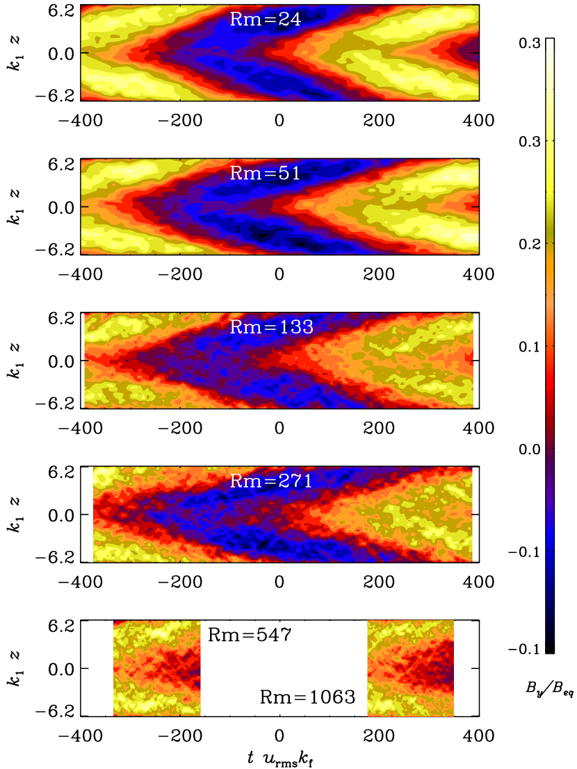
Figure 8: Space-time diagrams of $\overline{B}_{y}$ for wind $U_{0}=0.015c_{\rm s}$ (corresponding to ${\it S}_{\it W}\approx 0.0055$) for Models S1–S6 for different magnetic Reynolds numbers. From the top: ${{\rm Rm}}=24$, $51$, $133$, 271, as well as 547 (bottom left) and 1063 (bottom right).

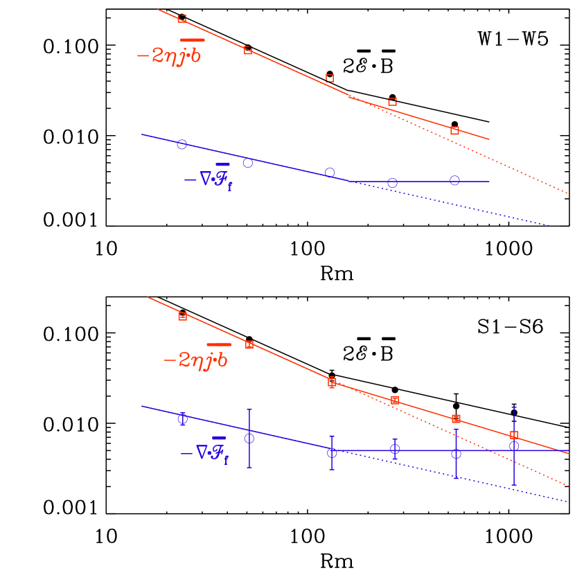
Figure 9: Scaling properties of the vertical slopes of $2\overline{\mbox{\boldmath${\cal E}$}}{}\cdot\overline{\bm{B}}$, $-2\eta\mu_{0}\,\overline{\bm{j}\cdot\bm{b}}$, and $-\mbox{\boldmath$\nabla$}{}\cdot\overline{\mbox{\boldmath${\cal F}$}}_{\rm f}{}$ for Models W1–W5 (upper panel) and for Models S1–S6 (lower panel). (Given that the three quantities vary approximately linearly with $z$, the three labels indicate their non-dimensional values at $k_{1}z=1$.) The second panel shows that for a stronger wind the contribution from the advective term becomes approximately independent of ${{\rm Rm}}$ for ${{\rm Rm}}>170$ (blue line), while that of the resistive term decreases approximately like ${{\rm Rm}}^{-2/3}$ (red line), and $2\overline{\mbox{\boldmath${\cal E}$}}{}\cdot\overline{\bm{B}}$ decreases approximately like ${{\rm Rm}}^{-1/2}$ (black line).

All simulations with wind show that the rms value of the mean field, $\overline{\bm{B}}_{\rm rms}$, declines slowly with increasing wind speed; see Figure 6. This result might just be a consequence of a gradual increase of the critical value of ${{\rm Rm}}$ above which dynamo action is possible. However, it could also be an indication that a fraction of the mean magnetic field is being removed from the domain by the flow – as found in the mean-field models of Shukurov et al. (2006).

In Figure 7 we see how $\overline{\bm{B}}_{\rm rms}$ decreases with increasing ${{\rm Rm}}$. The scalings ${{\rm Rm}}^{-0.4}$ and ${{\rm Rm}}^{-0.17}$ are given for orientation and show that in the presence of advection $\overline{\bm{B}}_{\rm rms}$ varies much slower than ${{\rm Rm}}^{-1}$, which is the slope anticipated from catastrophic quenching models without a wind (Brandenburg & Subramanian, 2005). Note, however, that DNS always gave a shallower slope (Brandenburg & Dobler, 2001) and, at larger values of ${{\rm Rm}}$, $\overline{\bm{B}}_{\rm rms}$ may have been already independent of ${{\rm Rm}}$ (Hubbard & Brandenburg, 2012). Indeed, without a wind (${\it S}_{\it W}=0$) the ${{\rm Rm}}$ dependence is compatible with a steeper ${{\rm Rm}}^{-1/2}$ law, but it is less certain in this case. Looking at Figure 8, we can also see that there is no significant change of the cycle period with ${{\rm Rm}}$. The high-resolution runs with ${{\rm Rm}}=544$ and 1061 are too short to cover a magnetic cycle, but one can see that the slope of the structure, which corresponds to the speed of the dynamo wave, is approximately unchanged. In the high-${{\rm Rm}}$ models the fluctuations are more pronounced, but the peak-to-peak contrast is about the same for all runs.

Table LABEL:simulation shows that $2\overline{\mbox{\boldmath${\cal E}$}}{}\cdot\overline{\bm{B}}$, $2\eta\mu_{0}\,\overline{\bm{j}\cdot\bm{b}}$, and $\mbox{\boldmath$\nabla$}{}\cdot\overline{\mbox{\boldmath${\cal F}$}}_{\rm f}{}$ balance approximately to zero, confirming that the results represent a statistically steady state. All three quantities have approximately the same (nearly linear) $z$ dependence for $|z|<L_{*}$, so that also the values of their three slopes must balance to zero, which is indeed the case. In Figure 9 we show the scaling properties of the aforementioned quantities for Models W1–W5 and S1–S6. For ${{\rm Rm}}\lesssim{{\rm Rm}_{\ast}}$, where ${{\rm Rm}_{\ast}}\approx 170$ for ${\it S}_{\it W}=0.002$ and ${{\rm Rm}_{\ast}}\approx 120$ for ${\it S}_{\it W}=0.005$, the first two quantities decrease approximatively like ${{\rm Rm}}^{-1}$, while the latter decreases only like ${{\rm Rm}}^{-1/2}$, which is in agreement with the values obtained by HB; see also Figure 10 of Candelaresi et al. (2011) for a corresponding plot.

Table 3: Additional parameters of the simulations including ${{\rm Rm}}$, magnetic diffusivity, the ratios ‘$\overline{\bm{B}}/u$’ ($=\overline{\bm{B}}_{\rm rms}/u_{\rm rms}$) and ‘$\overline{\bm{B}}/b$’ ($=\overline{\bm{B}}_{\rm rms}/b_{\rm rms}$), as well as Mach number and number of mesh points.

Model ${{\rm Rm}}$ $\eta k_{1}/c_{\rm s}$ ‘$\overline{\bm{B}}/u$’ ‘$\overline{\bm{B}}/b$’ $\rm Ma$ $N_{x}$ T1 $9$ $5.0\times 10^{-3}$ $0.58$ $1.13$ $0.18$ $64$ T2 $23$ $2.0\times 10^{-3}$ $0.48$ $0.87$ $0.19$ $64$ N1 $37$ $1.0\times 10^{-3}$ $0.53$ $0.70$ $0.15$ $64$ N2 $81$ $5.0\times 10^{-4}$ $0.58$ $0.73$ $0.16$ $128$ N3 $206$ $2.0\times 10^{-4}$ $0.27$ $0.33$ $0.17$ $256$ N4 $397$ $1.0\times 10^{-4}$ $0.27$ $0.33$ $0.16$ $512$ N5 $722$ $5.0\times 10^{-5}$ $0.18$ $0.21$ $0.15$ $1024$ N6 $1073$ $2.5\times 10^{-5}$ $0.11$ $0.15$ $0.11$ $1024$ W1 $24$ $1.0\times 10^{-3}$ $0.61$ $0.69$ $0.10$ $128$ W2 $51$ $5.0\times 10^{-4}$ $0.42$ $0.48$ $0.10$ $128$ W3 $129$ $2.0\times 10^{-4}$ $0.36$ $0.39$ $0.10$ $256$ W4 $265$ $1.0\times 10^{-4}$ $0.28$ $0.31$ $0.11$ $512$ W5 $540$ $5.0\times 10^{-5}$ $0.19$ $0.22$ $0.11$ $1024$ M2 $51$ $5.0\times 10^{-4}$ $0.36$ $0.45$ $0.10$ $128$ S1 $24$ $1.0\times 10^{-3}$ $0.40$ $0.55$ $0.10$ $64$ S2 $51$ $5.0\times 10^{-4}$ $0.31$ $0.42$ $0.10$ $128$ S3 $133$ $2.0\times 10^{-4}$ $0.20$ $0.27$ $0.11$ $256$ S4 $271$ $1.0\times 10^{-4}$ $0.17$ $0.23$ $0.11$ $512$ S5 $548$ $5.0\times 10^{-5}$ $0.15$ $0.19$ $0.11$ $1024$ S6 $1063$ $2.5\times 10^{-5}$ $0.14$ $0.17$ $0.11$ $1024$ I1 $26$ $1.0\times 10^{-3}$ $0.18$ $0.36$ $0.10$ $64$ I2 $55$ $5.0\times 10^{-4}$ $0.13$ $0.26$ $0.11$ $128$

However, for ${{\rm Rm}}\gtrsim 200$ the scaling of $2\overline{\mbox{\boldmath${\cal E}$}}{}\cdot\overline{\bm{B}}$ changes into an ${{\rm Rm}}^{-1/2}$ scaling; $\mbox{\boldmath$\nabla$}{}\cdot\overline{\mbox{\boldmath${\cal F}$}}_{\rm f}{}$ is at first below $2\eta\mu_{0}\,\overline{\bm{j}\cdot\bm{b}}$, but for high enough ${{\rm Rm}}$ increases to reach an absolute value similar to that of $2\overline{\mbox{\boldmath${\cal E}$}}{}\cdot\overline{\bm{B}}$. This suggests that the simple expectation based on the naive extrapolation given from a linear fit is misleading, and that catastrophic quenching might be alleviated already for ${{\rm Rm}}\gtrsim 1000$. In the absence of a wind and for large magnetic Reynolds numbers (Models N4–N6), the divergence of the magnetic helicity flux shows strong fluctuations about zero, making it harder to determine an accurate magnetic helicity balance of small-scale fields.

In Table LABEL:simulation2 we summarize additional output parameters of the simulations including ${{\rm Rm}}$, the magnetic diffusivity, the ratios of the rms values of mean field to fluctuating velocity and fluctuating magnetic field, i.e., $\overline{\bm{B}}_{\rm rms}/u_{\rm rms}$ and $\overline{\bm{B}}_{\rm rms}/b_{\rm rms}$, respectively, as well as Mach number and number of mesh points. As was already obvious from Figure 7, $\overline{\bm{B}}_{\rm rms}/u_{\rm rms}$ (which is the same as $\overline{\bm{B}}_{\rm rms}/B_{\rm eq}$), decreases with increasing ${{\rm Rm}}$, and the same is also true of the ratio $\overline{\bm{B}}_{\rm rms}/b_{\rm rms}$. The numerical resolution in the $x$ direction, $N_{x}$, is given in the last column. This is also the resolution used in the $y$ direction, while that in the $z$ direction is always twice as large.

4 Conclusions

In the present work we have examined the effects of an advective magnetic helicity flux in DNS of a turbulent dynamo. The present simulations without shear yield an oscillatory large-scale field owing to the spatially varying kinetic helicity profile with respect to the equatorial plane. We emphasize in this context that the possibility of oscillatory dynamos of $\alpha^{2}$ type is not new (Baryshnikova & Shukurov, 1987; Rädler & Bräuer, 1987), but until recently all known examples were restricted to spherical shell dynamos where $\alpha$ changes sign in the radial direction. The example found by Mitra et al. (2010b) applies to a spherical wedge with latitudinal variation of $\alpha$ changing sign about the equator. Similar results have also been obtained in a mean-field dynamo with a linear variation of $\alpha(z)\propto z$ (Brandenburg et al., 2009). Our present simulations are probably the first DNS of such a dynamo in Cartesian geometry. Closest to our simulations are those of MCCTB who used perfectly conducting outer boundary conditions without wind, and also found oscillatory solutions. Surprisingly, however, oscillations are here only obtained if there is at least a slight outflow.

One would have expected that catastrophic quenching can be alleviated if magnetic helicity is removed from the domain at a rate larger than its diffusion rate, that is, the advective term $\mbox{\boldmath$\nabla$}{}\cdot\overline{\mbox{\boldmath${\cal F}$}}_{\rm f}{}$ dominates over the resistive term, $2\eta\mu_{0}\,\overline{\bm{j}\cdot\bm{b}}$. Figure 9 shows that, for ${{\rm Rm}}\lesssim 200$, the latter term decreases linearly with decreasing $\eta$, while the former only decreases proportional to $\eta^{1/2}$, i.e., proportional to ${{\rm Rm}}^{-1/2}$. This would have led us to the estimate that for ${{\rm Rm}}\approx 4\cdot 10^{3}$ the catastrophic quenching can be alleviated by a wind with ${\it S}_{\it W}\approx 0.005$. Our new results suggest that this can happen already for smaller values of ${{\rm Rm}}$. The reason for this is still unclear. It is possible that catastrophic quenching was an artefact of intermediate values of ${{\rm Rm}}$, as suggested by Hubbard & Brandenburg (2012), or that a magnetic helicity flux can have an effect even though it is weak compared with diffusive terms.

Finally, we should emphasize that we have only examined here the case of subsonic advection. In real astrophysical cases, like galactic and stellar winds, the outflow is instead supersonic and can, thus, play an even more important role in alleviating the catastrophic quenching through the advection of magnetic helicity. This assumes, of course, that the dynamo is strong enough to be still excited in the presence of a stronger wind.

References

- Baryshnikova & Shukurov (1987) Baryshnikova I., Shukurov A., 1987, Astron. Nachr., 308, 89
- Brandenburg (2001) Brandenburg A., 2001, ApJ, 550, 824
- Brandenburg et al. (2009) Brandenburg A., Candelaresi S., Chatterjee P., 2009, MNRAS, 398, 1414
- Brandenburg & Dobler (2001) Brandenburg A., Dobler W., 2001, A&A, 369, 329
- Brandenburg et al. (2002) Brandenburg A., Dobler W., Subramanian K., 2002, Astron. Nachr., 323, 99
- Brandenburg et al. (1995) Brandenburg A., Nordlund Å., Stein R. F., & Torkelsson U., 1995, ApJ, 446, 741
- Brandenburg & Subramanian (2005) Brandenburg A., Subramanian K., 2005, Astron. Nachr., 326, 400
- Candelaresi et al. (2011) Candelaresi S., Hubbard A., Brandenburg A., Mitra D., 2011, Phys. Plasmas, 18, 012903
- Cattaneo & Hughes (1996) Cattaneo F., Hughes D. W., 1996, Phys. Rev. E, 54, 4532
- Chatterjee et al. (2011) Chatterjee P., Guerrero G., Brandenburg A., 2011, A&A, 525, A5
- Gruzinov & Diamond (1994) Gruzinov A. V., Diamond P. H., 1994, Phys. Rev. Lett., 72, 1651
- Guerrero et al. (2010) Guerrero G., Chatterjee P., Brandenburg A., 2010, MNRAS, 409, 1619
- Hubbard & Brandenburg (2010) Hubbard A., Brandenburg A., 2010, Geophys. Astrophys. Fluid Dyn., 104, 577 (HB)
- Hubbard & Brandenburg (2011) Hubbard A., Brandenburg A., 2011, ApJ, 727, 11
- Hubbard & Brandenburg (2012) Hubbard A., Brandenburg A., 2012, ApJ, 748, 51
- Käpylä et al. (2008) Käpylä P. J., Korpi M. J., Brandenburg A., 2008, A&A, 491, 353
- Käpylä et al. (2009) Käpylä P. J., Korpi M. J., Brandenburg A., 2009, A&A, 500, 633
- Käpylä et al. (2010) Käpylä P. J., Korpi M. J., Brandenburg A., 2010, A&A, 518, A22
- Kleeorin et al. (2000) Kleeorin N., Moss D., Rogachevskii I., Sokoloff D., 2000, A&A, 361, L5
- Kleeorin & Ruzmaikin (1982) Kleeorin N. I., Ruzmaikin A. A., 1982, Magnetohydrodynamics, 18, 116
- Krause & Rädler (1980) Krause F., Rädler K., 1980, Mean-field magnetohydrodynamics and dynamo theory. Pergamon Press, Oxford
- Mitra et al. (2010a) Mitra D., Candelaresi S., Chatterjee P., Tavakol R., Brandenburg A., 2010a, Astron. Nachr., 331, 130 (MCCTB)
- Mitra et al. (2010b) Mitra D., Tavakol R., Käpylä P. J., Brandenburg A., 2010b, ApJL, 719, L1
- Mitra et al. (2011) Mitra D., Moss D., Tavakol R., Brandenburg A., 2011, A&A, 526, A138
- Moffatt (1978) Moffatt H. K., 1978, Magnetic field generation in electrically conducting fluids. Cambridge Univ. Press, Cambridge
- Pouquet et al. (1976) Pouquet A., Frisch U., Leorat J., 1976, J. Fluid Mech., 77, 321
- Rädler & Bräuer (1987) Rädler K.-H., Bräuer H.-J., 1987, Astron. Nachr., 308, 101
- Shukurov et al. (2006) Shukurov A., Sokoloff D., Subramanian K., Brandenburg A., 2006, A&A, 448, L33
- Sur et al. (2008) Sur S., Brandenburg A., Subramanian K., 2008, MNRAS, 385, L15
- Sur et al. (2007) Sur S., Shukurov A., Subramanian K., 2007, MNRAS, 377, 874
- Vainshtein & Cattaneo (1992) Vainshtein S. I., Cattaneo F., 1992, ApJ, 393, 165
- Vishniac & Cho (2001) Vishniac E. T., Cho J., 2001, ApJ, 550, 752
- Warnecke et al. (2011) Warnecke J., Brandenburg A., Mitra D., 2011, A&A, 534, A11