Representations of solutions of the wave equation based on relativistic wavelets

Abstract

A representation of solutions of the wave equation with two spatial coordinates in terms of localized elementary ones is presented. Elementary solutions are constructed from four solutions with the help of transformations of the affine Poincaré group, i.e., with the help of translations, dilations in space and time and Lorentz transformations. The representation can be interpreted in terms of the initial-boundary value problem for the wave equation in a half-plane. It gives the solution as an integral representation of two types of solutions: propagating localized solutions running away from the boundary under different angles and packet-like surface waves running along the boundary and exponentially decreasing away from the boundary. Properties of elementary solutions are discussed. A numerical investigation of coefficients of the decomposition is carried out. An example of the field created by sources moving along a line with different speeds is considered, and the dependence of coefficients on speeds of sources is discussed.

¹ Department of Mathematical Physics, Physics Faculty, St.Petersburg University, Ulyanovskaya 1-1, Petrodvorets, St.Petersburg, 198904, Russia

² Ioffe Physical-Technical Institute of the Russian Academy of Sciences
26 Polytekhnicheskaya, St Petersburg 194021, Russia

perel@mph.phys.spbu.ru

1 Introduction

The construction of exact representations of solutions of the wave equation in terms of elementary localized solutions is the subject of the present paper. Fourier analysis yields a representation of solutions in terms of plane waves. An analogue of Fourier analysis in our considerations is continuous wavelet analysis. We use here a special version of continuous wavelet analysis based on the transformations of the affine Poincaré group [1] (Wavelets based on the Poincaré group was discussed also in [2], [3].) The representation obtained by us is associated with the initial-boundary value problem in the half-plane. It is given in terms of the affine Poincaré wavelet transform of time-dependent boundary data on a line, which is the boundary of the half-plane. The wavelet transform is efficient in processing of functions of time and coordinate, which are results of observations and which have a multiscale structure [1]. The result of propagation of data is given by us in terms appropriate for data processing.

The representations of solutions of the non-stationary wave equation as superpositions of elementary localized solutions have been presented for the first time in the work of Kaiser [4]. They were based on the analytic wavelet transform, and he used very special spherically symmetric elementary solutions. Representations of solutions in terms of elementary solutions from a wide class were proposed in [5], [6], [7] and discussed in [8]. That representation was based on continuous wavelet analysis. Elementary solutions are constructed from two chosen ones by means of a similitude group of transformations that contains shifts, scalings, and rotations. In present work, a solution of the non-stationary boundary problem for the wave equation has been decomposed in localized elementary solutions by means of the space-time version of wavelet analysis. Elementary solutions are constructed from four chosen ones by means of an affine Poincaré group of transformations that contains shifts and scaling both in space and in time and the Lorentz transformations. Preliminary results were reported in [9]. The affine Poincaré wavelet transform (APWT) is a coefficient in the decomposition of solutions. The region of integration is determined by the values of parameters under which the APWT is above a certain level. Numerical implementation and examples of calculation of APWT were discussed in our work [10].

For the sake of simplicity we consider here only the case of two spacial dimensions.

In section 2, we recall affine Poincaré wavelet transform theory. In section 3, we develop Poincaré wavelet theory for solutions and construct representations of solutions of the wave equation based on it. Then we give examples of mother solutions and discuss properties of elementary solutions obtained from them. The implementation and interpretation of Poincaré wavelet transform are considered in section 5 with several examples.

We suggest to determine mother wavelets by means of their Fourier integrals which has not explicit form in the coordinate domain. However we may take as mother solutions exact particle-like solutions found in [11], [12], [13], [14] which are given by simple explicit formulas both in the coordinate and in the Fourier domains. The review of another exact localized solutions is done in [15], [16]. Solutions obtained by Lorentz transformations are discussed in [17].

A representation obtained of solutions can find applications in the non-stationary diffraction theory, in the propagation and scattering of multiscale fields, for example, in seismology. We hope that our results may be useful also in astronomy to determine velocities of relativistic objects or to deal with time-dependent problems of scattering.

2 Basics of affine Poincaré wavelet analysis

First steps in the application of wavelet analysis methods are the definition of a class of functions ${\cal H}$ considered, a choice of a mother wavelet $\psi\in{\cal H},$ and the construction of a family of wavelets. The mother wavelet is a fixed function. A family of wavelets is functions obtained from the mother wavelet by means of transformations of a group. The set of wavelets should be dense in the chosen space ${\cal H}$. Then it should be proved that any function $f\in{\cal H}$ can be represented as an integral superposition of wavelets.

It is useful to consider together functions and their Fourier transforms. Below we introduce the notation

$$\boldsymbol{\chi}=\binom{ct}{x},\quad\boldsymbol{\sigma}=\binom{\omega/c}{k_{x}},$$ (1)

and define the Minkovsky inner product as follows: $(\boldsymbol{\sigma},\boldsymbol{\chi})=-\omega t+k_{x}x$. The method of wavelet analysis itself is not associated with the wave equation. We apply it to the boundary data function $f(\boldsymbol{\chi})\equiv f(ct,x)$ dependent only on one spatial coordinate $x$ and time $t.$ The Fourier transform of any $f(\boldsymbol{\chi})\in\mathbb{L}_{2}$ reads

$$\hat{f}(\boldsymbol{\sigma})=\int\limits_{\mathbb{R}^{2}}d^{2}\boldsymbol{\chi}\,f(\boldsymbol{\chi})e^{-i(\boldsymbol{\sigma},\boldsymbol{\chi})}.$$ (2)

Lorentz transformations enables one to connect the coordinate $x$ and the time $t$ in a stationary coordinate system with the coordinate $x^{\prime}$ and the time $t^{\prime}$ in a moving one with speed $v$. It reads

$$\binom{ct^{\prime}}{x^{\prime}} =\Lambda_{\phi}\binom{ct}{x},$$ (3)

$$\Lambda_{\phi} =\left(\begin{array}[]{cc}\cosh\phi&-\sinh\phi\\ -\sinh\phi&\cosh\phi\end{array}\right),\tanh\phi=\frac{v}{c},$$ (6)

where $\phi$ is called the rapidity and $v$ is the speed of the moving frame. The frequency and the wave number in the moving frame and in the stationary frame given by vectors $\boldsymbol{\sigma}^{\prime}$ and $\boldsymbol{\sigma},$ respectively, are related as $\boldsymbol{\sigma}^{\prime}=\Lambda_{-\phi}\boldsymbol{\sigma}.$

We are going to clarify the choice of the space ${\cal H}.$ We choose any $\psi(ct,x)\in\mathbb{L}_{2}$. Construct a family of wavelets with transformations of the affine Poincaré group, i.e., with shifting, scaling and the Lorentz transformations:

$$\psi_{\mu}(\boldsymbol{\chi})=\frac{1}{a}\psi\left(\Lambda_{-\phi}\frac{\boldsymbol{\chi}-\boldsymbol{b}}{a}\right)\,,\boldsymbol{b}=\binom{c\tau}{b_{x}}\,,$$ (7)

$$\mu=\{\boldsymbol{b},a,\phi\}.\,$$ (8)

A wavelet $\psi_{\mu}(\boldsymbol{\chi})$ for $a=1,$ $\boldsymbol{b}=0$ represents a wave packet in the stationary frame, such that it is the mother wavelet in the moving frame. The constructed family is not dense in the whole $\mathbb{L}_{2}.$ To show this, we analyze the Fourier transform of wavelets

$$\widehat{\psi_{\mu}}(\boldsymbol{\sigma})=a\widehat{\psi}(a\Lambda_{-\phi}\boldsymbol{\sigma})e^{-i(\boldsymbol{\sigma},\boldsymbol{b})}\,$$ (9)

and show that we cannot go beyond the region bounded by the lines $\omega=\pm ck_{x}$ under the action of Lorentz transformations. For example, a point from the domain $k>0,|k_{x}|<k$ cannot be mapped to any point in the domain $k_{x}>0,|k|<k_{x},$ by choosing $a$ and $\phi$.

The explanation of this fact is below. Let the support of the Fourier transform of the mother wavelet in the moving frame be concentrated near a point $\boldsymbol{\sigma}_{0}^{\prime},$ i.e., $\hat{\psi}(\boldsymbol{\sigma}^{\prime})\equiv 0$ outside a neighborhood of $\boldsymbol{\sigma}_{0}^{\prime}.$ The support of this packet in the stationary frame lies in the neighborhood of $\boldsymbol{\sigma}_{0},$ such that $\boldsymbol{\sigma}_{0}=a^{-1}\Lambda_{\phi}\boldsymbol{\sigma}^{\prime}_{0}.$ It is easy to check that the point $(\omega_{0}/c,k_{x0})$ lies on the hyperbola $(\omega_{0}/c)^{2}-k_{x0}^{2}=a^{-2}((\omega_{0}^{\prime}/c)^{2}-k_{x0}^{{}^{\prime}2}).$ For any prescribed $(\omega_{0},k_{x0})$ we can find a unique parameter $a>0.$ The parameter $\phi$ can be found by the relation $\tanh(\phi+\phi^{\prime})=ck_{x0}/\omega_{0},$ where $\tanh(\phi^{\prime})=ck^{\prime}_{x}/\omega^{\prime}.$ As $\phi$ increases, the point $(\omega_{0}/c,k_{x0})$ tends to the asymptotes of the hyperbola $\omega=\pm ck_{x}$. Let $\omega_{0}^{\prime}>0,$ $c|k_{x0}^{\prime}|<\omega_{0}^{\prime}$. Then for any $a$ and $\phi$ the point $(\omega_{0}/c,k_{x0})$ lies in the same region: $\omega_{0}>0,$ $c|k_{x0}|<\omega_{0}$.

Therefore we should decompose the space ${\mathbb{L}}_{2}(\mathbb{R}^{2})$ into a direct sum: ${\mathbb{L}}_{2}(\mathbb{R}^{2})=\bigoplus\limits_{j=1}^{4}{\cal{H}}_{j}$ taking into account their Fourier transforms. The space ${\cal{H}}_{j}$ comprises functions $f_{j}\in{\mathbb{L}}_{2}(\mathbb{R}^{2}),$ which have the support of their Fourier transform in ${\cal{D}}_{j}$ (see fig.1) :

$$f_{j}(\boldsymbol{\chi})=\frac{1}{(2\pi)^{2}}\int\limits_{{\cal{D}}_{j}}d^{2}\boldsymbol{\sigma}\,\hat{f}(\boldsymbol{\sigma})e^{i(\boldsymbol{\sigma},\boldsymbol{\chi})}\,.$$ (10)

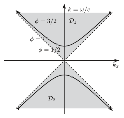
(a) Domains ${\cal{D}}_{1}$ and ${\cal{D}}_{2}$

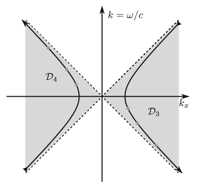
(b) Domains ${\cal{D}}_{3}$ and ${\cal{D}}_{4}$

Figure 1: Domains ${\cal{D}}_{j}$ that are supports of the Fourier transform of functions from ${\cal{H}}_{j}$, $j=1,2,3,4$. The set of points obtained by Lorentz transformations from the point with $\phi=0$ is a hyperbola. Arrows on hyperbolas show the direction of point movement from $\phi=-\infty$ to $\phi=+\infty.$

The mother wavelet is any function $\psi_{j}(\boldsymbol{\chi})\in{\cal{H}}_{j}$ that satisfies an admissibility condition:

$$C_{j}=\int\limits_{{\cal{D}}_{j}}d^{2}\boldsymbol{\sigma}\,\frac{|\hat{\psi}_{j}(\boldsymbol{\sigma})|^{2}}{|(\omega/c)^{2}-k^{2}_{x}|}<\infty.$$ (11)

The family of wavelets is constructed by formulas (7).

The affine Poincaré wavelet transform $F_{j}(\mu)$ of the function $f_{j}$ is defined as follows [1]:

$$F_{j}(\mu)=\int\limits_{\mathbb{R}^{2}}d^{2}\boldsymbol{\chi}\,f_{j}(\boldsymbol{\chi})\overline{\psi_{j\mu}(\boldsymbol{\chi})},\quad\mu=\{\boldsymbol{b},a,\phi\}.$$ (12)

We denote functions from $\mathbb{L}_{2}$ by Latin lowercase letters and their wavelet transforms by Latin uppercase letters. It is not necessary to extract $f_{j}(\boldsymbol{\chi})$ from $f(\boldsymbol{\chi})$ to calculate $F_{j}(\mu)$, as follows from the Plancherel equality:

$$(f_{j},\psi_{j\mu})=\frac{1}{(2\pi)^{2}}(\hat{f}_{j},\hat{\psi}_{j\mu})=\frac{1}{(2\pi)^{2}}(\hat{f},\hat{\psi}_{j\mu})=(f,\psi_{j\mu}).$$ (13)

The main fact that yields the decomposition of solutions is the Plancherel equality for the affine Poincaré wavelet transform [1]:

$$(f_{j},g_{j})_{\mathbb{L}_{2}}=\frac{1}{{C_{j}}}\int d\mu\,F_{j}(\mu)\overline{G_{j}(\mu)},$$ (14)

where

$$\int d\mu\equiv{\int\limits_{\mathbb{R}}d\phi}{\int\limits_{0}^{\infty}\frac{da}{{a^{3}}}}{\int\limits_{\mathbb{R}^{2}}d^{2}\boldsymbol{b}}.$$ (15)

Equality (14) is valid for any $f_{j},g_{j}\in{\cal H}_{j}$ if the admissibility condition (11) is fulfilled.

The reconstruction formula following from the Plancherel equality reads

$$f_{j}(\boldsymbol{\chi})=\frac{1}{{C_{j}}}\int d\mu\,F_{j}(\mu)\psi_{j\mu}(\boldsymbol{\chi}).$$ (16)

See the A for more detail. Any $f(\boldsymbol{\chi})\in\mathbb{L}_{2}$ can be represented as $f(\boldsymbol{\chi})=\sum\limits_{j=1}^{4}f_{j}(\boldsymbol{\chi}).$

3 Decomposition of solutions

In the present section we give exact decompositions of solutions of the wave equation based on the formulas discussed above. The decomposition is associated with the boundary problem for the wave equation in a half-plane $y\geq 0$, $-\infty<x<\infty$:

$$u_{tt}=c^{2}(u_{xx}+u_{yy})$$ (17)

$$u(ct,x,y)\left.\right|_{y=0}=f(ct,x),$$ (18)

$$u(ct,x,y)\left.\right|_{t\leq 0}=0.$$ (19)

where $c$ is the speed, $t$ is time, $x$ and $y$ are spatial variables. The function $f(ct,x)$ in (18) is assumed to be square integrable:

$$\int\limits_{\mathbb{R}}d(ct)\int\limits_{\mathbb{R}}dx\,|f(ct,x)|^{2}<\infty.$$ (20)

The desired decomposition is expressed in terms of solutions running away from the boundary under different angles. It was first reported in [9].

We define four subspaces of solutions $\mathfrak{H}_{j},$ $j=1,\ldots,4$ of the wave equation using the Fourier transform of the boundary data $\hat{f}(\boldsymbol{\sigma})$. Any function $u_{j}(\boldsymbol{\chi},y)\in\mathbb{L}_{2}$ belongs to $\mathfrak{H}_{j}$ if its Fourier decomposition reads

$$u_{j}(\boldsymbol{\chi},y)=\int\limits_{{\cal D}_{j}}d^{2}\sigma\,\hat{f}(\boldsymbol{\sigma})e^{i(\boldsymbol{\sigma},\boldsymbol{\chi})}e^{i\sqrt{k^{2}-k_{x}^{2}}y},\quad j=1,2,$$ (21)

$$u_{j}(\boldsymbol{\chi},y)=\int\limits_{{\cal D}_{j}}d^{2}\sigma\,\hat{f}(\boldsymbol{\sigma})e^{i(\boldsymbol{\sigma},\boldsymbol{\chi})}e^{-\sqrt{k_{x}^{2}-k^{2}}y},\quad j=3,4,$$ (22)

where $k=\omega/c$ is the wave number for any $\hat{f}(\boldsymbol{\sigma})\in\mathbb{L}_{2}$. The functions $u_{j}(\boldsymbol{\chi},y),j=1,\ldots,4,$ are solutions of the wave equation. If a function $\hat{f}(\boldsymbol{\sigma})$ decreases at infinity not so slowly to produce a classical solution, the functions $u_{j}(\boldsymbol{\chi},y)$ satisfy the wave equation in the distribution sense. The solutions $u_{j}(\boldsymbol{\chi},y),j=1,2,$ are propagating, the solutions $u_{j}(\boldsymbol{\chi},y),j=3,4,$ are exponentially decreasing and associated with details of the spatial behavior of $f,$ which are smaller than the wavelength. Note that the reconstruction formula for the Fourier transform yields $\sum\limits_{j=1}^{4}u_{j}(\boldsymbol{\chi},0)=f(\boldsymbol{\chi}).$

In what follows we will use the Fourier transforms of solutions with respect to $t$ and $x$ denoted by $\hat{u}_{j}(\boldsymbol{\sigma};y)$ :

$$\hat{u}_{j}(\boldsymbol{\sigma};y) =\hat{f}(\boldsymbol{\sigma})e^{i\sqrt{k^{2}-k_{x}^{2}}y},j=1,2,$$ (23)

$$\hat{u}_{j}(\boldsymbol{\sigma};y) =\hat{f}(\boldsymbol{\sigma})e^{-\sqrt{k_{x}^{2}-k^{2}}y},j=3,4.$$ (24)

The Fourier transforms of solutions with respect to $x$ and $y$ dependent on $t$ are denoted by $\hat{u}_{j}(ct;k_{x},k_{y})$:

$$\hat{u}_{j}(ct;k_{x},k_{y}) =\hat{f}(\boldsymbol{\sigma})e^{-i\omega t},j=1,2,\quad\boldsymbol{\sigma}=(\sqrt{k_{x}^{2}+k_{y}^{2}},k_{x})^{\top}.$$ (25)

The solutions ${u}_{j}(ct,x,y),$ $j=3,4,$ increase exponentially for negative $y$. The Fourier transform of them with respect to $x$ and $y$ do not exist.

To develop a procedure of continuous wavelet analysis in the subspace $\mathfrak{H}_{j},$ we should choose a solution $\Psi_{j}\in\mathfrak{H}_{j}.$ We call it the mother solution. The notation of the mother solution begins with the Greek uppercase letter and that distinguishes it from the mother wavelet in $\mathbb{L}_{2},$ which is denoted by the Greek lowercase letter. The mother solution can be reduced to the mother wavelet if $y=0$. Therefore $\psi_{j}(\boldsymbol{\chi})=\Psi_{j}(\boldsymbol{\chi},0)$ should satisfy the admissibility condition (11).

Then we construct a family of solutions:

$$\Psi_{j\mu}(\boldsymbol{\chi},y)=\frac{1}{a}\Psi_{j}\left(\Lambda_{-\phi}\frac{\boldsymbol{\chi}-\boldsymbol{b}}{a},\,\frac{y}{a}\right).$$ (26)

Each solution represents a wave packet considered in the stationary frame, which is a shifted and scaled mother solution in the frame moving in the $x$ direction. These solutions are transformed to wavelets from the family (7) on the line $y=0$, i.e., $\Psi_{j\mu}(\boldsymbol{\chi},0)\equiv\psi_{j\mu}(\boldsymbol{\chi}),$ where $\psi_{j\mu}(\boldsymbol{\chi})$ are wavelets.

The decomposition of solutions of (17) in terms of mother wavelets read

$$u(\boldsymbol{\chi},y)=\sum\limits_{j=1}^{4}u_{j}(\boldsymbol{\chi},y),\quad u_{j}(\boldsymbol{\chi},y)=\frac{1}{{C_{j}}}\int d\mu\,F_{j}(\mu)\Psi_{j\mu}(\boldsymbol{\chi},y),$$ (27)

$$F_{j}(\mu)=\int\limits_{\mathbb{R}^{2}}d^{2}\boldsymbol{\chi}\,f(\boldsymbol{\chi})\overline{\Psi_{j\mu}(\boldsymbol{\chi},0)}.$$ (28)

It is a solution because it is a decomposition of solutions. It is reduced to the reconstruction formula for the boundary data $f$ if $y=0$ and therefore it satisfies the boundary conditions. Each of solutions moves or decreases away from the boundary. We do not take into account solutions that come from infinity and increase in the positive $y$ direction to satisfy initial conditions (19) .

The contribution of each solution is determined by the coefficient $F_{j},$ which is the wavelet transform of the boundary data.

4 Examples of mother solutions

Mother solutions can be taken from a wide class. We give examples of mother solutions, which behave as particles. As a starting point we take a solution that has the Fourier transform localized near the point $k_{x}=0,$ $k_{y}=\varkappa:$

$$\hat{\Psi}(ct;k_{x},k_{y})=\exp{\left(-\frac{\sigma_{\parallel}^{2}(k_{y}-\varkappa)^{2}}{2}-\frac{\sigma_{\perp}^{2}k_{x}^{2}}{2}\right)}e^{-i\omega t},$$ (29)

where $\omega=c|\boldsymbol{k}|.$ If $t=0$, then the solution in the coordinate domain reads

$$\Psi(0,x,y)=\frac{1}{2\pi\sigma_{\parallel}\sigma_{\perp}}\exp{\left({i}\varkappa y-\frac{y^{2}}{2\sigma_{\parallel}^{2}}-\frac{x^{2}}{2\sigma_{\perp}^{2}}\right)}.$$ (30)

If $t\neq 0$, the solution cannot be found explicitly. But if $t$ is small enough, then $\Psi_{1}(ct,x,y)\approx\Psi_{1}(0,x,y-ct).$ It can be obtained by expanding $k=\sqrt{k_{x}^{2}+k_{y}^{2}}$ up to linear terms: $\omega=\omega_{0}+c(k_{y}-\varkappa)+\ldots$ and substituting it into the phase:

$$k_{x}x+k_{y}y-\omega t={k_{x}}x+k_{y}(y-ct)+\ldots.$$

On this way, for small time we obtain a packet-like solution which is filled with oscillations of a spatial frequency $\varkappa$ and which has the Gaussian envelope. It moves along the $y$ axis with speed $c$.

For large $t$ the solution should be found numerically. Exact solutions having similar local behavior were found in [12] and were named ’Gaussian wave packets’. Solutions and their Fourier transforms were given by explicit formulas and were studied analytically. An investigation of these solutions from the point of view of continuous wavelet analysis was performed in [14].

To be a mother solution in $\mathfrak{H}_{1},$ this solution should contain Fourier components with $\omega>0$ and $k_{y}>0$. The last condition is fulfilled only approximately if the central frequency of the packet $\varkappa$ is larger than the width of the support of the Fourier transform in $k_{y}$ direction $1/\sigma_{\parallel}$, i.e. $\varkappa\sigma_{\parallel}=\sqrt{p}>>1$. To obtain the mother solution, we assume that formula (29) is valid only for $k_{y}>0$ and $\hat{\Psi}(ct;kx,ky)=0$ if $k_{y}\leq 0.$ To make the Fourier transform smooth, we introduce an additional factor $\exp{(-\frac{1}{k_{y}})},k_{y}=\sqrt{k^{2}-k_{x}^{2}}.$ The mother solution $\Psi_{1}(ct,x,y)$ is of the form

$$\Psi_{1}(ct,x,y)=\frac{1}{(2\pi)^{2}}\int\limits_{-\infty}^{\infty}dk_{x}\int\limits_{0}^{\infty}dk_{y}\,\exp\left(-\frac{\sigma_{\parallel}^{2}(k_{y}-\varkappa)^{2}}{2}-\frac{\sigma_{\perp}^{2}k_{x}^{2}}{2}\right)$$ (31)

$$\exp(-1/k_{y})\exp\left(i(k_{x}x+k_{y}y-kct)\right),$$

$k=|\boldsymbol{k}|.$ Because of the factor $\exp{(-{1}/{k_{y}})}$, the solution satisfies the admissibility condition. We take a variable of integration $k=\sqrt{k_{x}^{2}+k_{y}^{2}}$ instead of $k_{y}$ and write the Fourier transform of (31) in the form of (23). Then we obtain

$$\widehat{\Psi}_{1}(\boldsymbol{\sigma};y)=\frac{k}{k_{y}}\exp\left(-\frac{\sigma_{\parallel}^{2}(k_{y}-\varkappa)^{2}}{2}-\frac{\sigma_{\perp}^{2}k_{x}^{2}}{2}-\frac{1}{k_{y}}\right)\cdot e^{ik_{y}y},$$ (32)

$k_{y}=\sqrt{k^{2}-k_{x}^{2}}$. Fig.2a shows this solution in successive time moments. It represents a wave packet moving away from the boundary $y=0$. It has a finite energy, because it is localized in an exponential way. The same solution for other choice of parameters in the case $\varkappa\sigma_{\parallel}=\sqrt{p}=2$ is shown in Fig.3a.

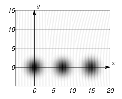
(a) Solutions in the moving frame

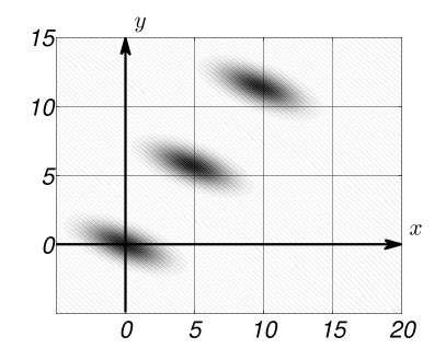
(b) Same solutions in the stationary frame, $\phi=1$

Figure 2: Real part of mother wavelet $\Psi_{1}$ with parameters $\varkappa=16$, $\sigma_{\parallel}=\sqrt{2}$, $\sigma_{\perp}=\sqrt{2}$ in successive time moments: $ct=0$, $ct=7.5$, $ct=15$.

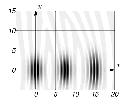
(a) Solutions in the moving frame

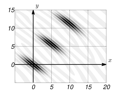
(b) The same solutions in the stationary frame, $\phi=1$

Figure 3: Real part of the mother wavelet $\Psi^{1}$ with parameters $\varkappa=4$, $\sigma_{\parallel}=1$, $\sigma_{\perp}=2$ in successive time moments: $ct=0$, $ct=7.5$, $ct=15$.

The mother solution in $\mathfrak{H}_{3}$ is constructed in a similar way. We interchange $k$ and $k_{x},$ put $iy$ instead of $y,$ and obtain

$$\hat{\Psi}_{3}(\boldsymbol{\sigma};y)=\frac{k_{x}}{\sqrt{k_{x}^{2}-k^{2}}}\exp\left(-\frac{\sigma_{\parallel}^{2}(\sqrt{k_{x}^{2}-k^{2}}-\varkappa)^{2}}{2}-\frac{\sigma_{\perp}^{2}k^{2}}{2}\right)$$ (33)

$$\exp\left(-1/\sqrt{k_{x}^{2}-k^{2}}\right)\cdot e^{-\sqrt{k_{x}^{2}-k^{2}}y}.$$

The solution $\Psi_{3}(ct,x,y)$ is a wave packet running along the boundary and decreasing exponentially in the positive $y$ direction. The Fourier transform of the solution comprises components with wavelengths in the $x$ direction, which are smaller than the wavelength in vacuum. Fig.4a demonstrates the solution in successive time moments. The wavelet analysis of solutions from $\mathfrak{H}_{3}$ and $\mathfrak{H}_{4}$ might be useful for analyzing of surface waves, but a more detail study of the problem goes beyond the scope of this paper.

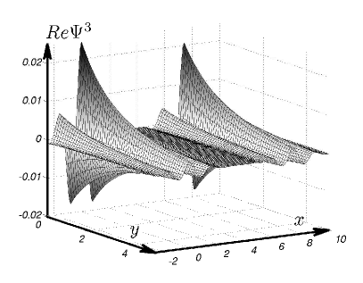
(a) Solutions in the moving frame

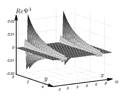
(b) The same solutions in the stationary frame, $\phi=1$

Figure 4: Real part of the mother wavelet $\Psi_{3}$ with parameters $\varkappa=4$, $\sigma_{\parallel}=1$, $\sigma_{\perp}=2$ in successive time moments: $ct=0$ and $ct=7.5$.

The mother solutions in $\mathfrak{H}_{2}$ and $\mathfrak{H}_{4}$ can be obtained as follows: $\Psi_{2}(ct,x,y)=\Psi_{1}(-ct,x,y),$ $\Psi_{4}(ct,x,y)=\Psi_{3}(ct,-x,y).$

Now we discuss analytically the properties of the family of solutions obtained by means of Lorentz transformations. The mother solution $\Psi_{1}(ct,x,y)$ represents a wave packet moving in the positive $y$ direction and localized near the point $x=0$, $y=ct$. In the Fourier domain, it is localized near the point $\sigma_{0}=(\varkappa,0),$ $\omega_{0}=c\varkappa.$ Now consider $\Psi_{1}(ct^{\prime},x^{\prime},y),$ where $x^{\prime},y,t^{\prime}$ are coordinates in the frame that moves with speed $v$ and rapidity $\phi.$ The coordinates in the moving frame are connected with the coordinates in the stationary frame by transformations (3). Assuming that $t^{\prime}$ is small enough, we obtain $\Psi_{1}(ct^{\prime},x^{\prime},y)\approx\Psi_{1}(0,x^{\prime},y-ct^{\prime})=\Psi_{1}(0,\cosh\phi(x-ct\tanh\phi),y+\sinh\phi x-\cosh\phi ct).$ The position of the center of the packet $x_{0},y_{0}$ in the stationary frame is $x_{0}=ct\tanh\phi,$ $y_{0}=ct/\cosh\phi.$ The packet (31) found in the moving frame is numerically small outside an ellipse

$$\frac{(y-ct^{\prime})^{2}}{2\sigma_{\parallel}^{2}}+\frac{x^{\prime 2}}{2\sigma_{\perp}^{2}}\leq 1$$ (34)

For the sake of simplicity we assume that it is a circle $\sigma\equiv\sigma_{\parallel}=\sigma_{\perp}$:

$$(x^{\prime})^{2}+(y-ct^{\prime})^{2}\leq 2\sigma^{2}.$$ (35)

An example of such a solution is shown in Fig.2a. Taking into account (3) we find the domain in the stationary frame corresponding to the circle (35) in the moving frame. It is an ellipse:

$$\cosh^{2}\phi(x-x_{0})^{2}+((y-y_{0})-\sinh\phi(x-x_{0}))^{2}\leq 2\sigma^{2}.$$ (36)

This ellipse in the main axes reads

$$\lambda_{1}\tilde{x}^{2}+\lambda_{2}\tilde{y}^{2}\leq 2\sigma^{2}.$$ (37)

where

$$\lambda_{1,2}=e^{\pm\phi}\cosh\phi.$$ (38)

The directions of the main axes are

$$\boldsymbol{e_{1,2}}=\left(\begin{array}[]{c}\pm e^{\mp\phi}\\ 1\end{array}\right).$$ (39)

The new coordinates $\tilde{x}$, $\tilde{y}$ are connected with the old coordinates $x-x_{0},$ $y-y_{0}$ by the relation

$$\binom{\tilde{x}}{\tilde{y}}=U^{\top}\binom{x-x_{0}}{y-y_{0}},\quad U=\left(\frac{\boldsymbol{e}_{1}}{|\boldsymbol{e}_{1}|},\frac{\boldsymbol{e}_{2}}{|\boldsymbol{e}_{2}|}\right),$$ (40)

where the columns of the matrix $U$ are vectors $\boldsymbol{e_{j}},j=1,2.$

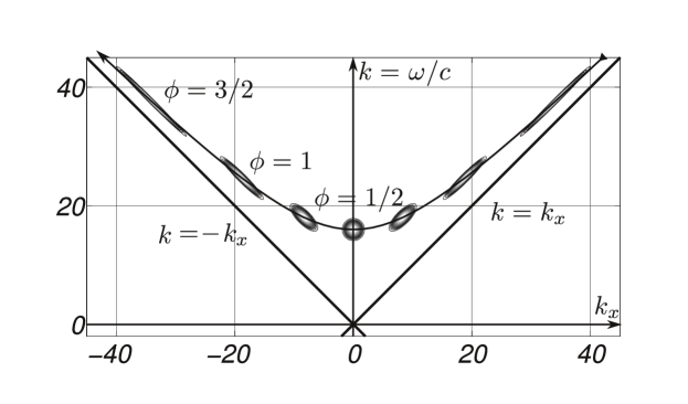
Figure 5: The support of the wavelet in the Fourier domain for various $\phi$

The axes of the ellipse in the stationary frame are not orthogonal to the direction of propagation and to wave fronts (see Fig.2).

Similar considerations are valid in the Fourier domain. The support of the Fourier transform of the solution is distorted under the action of the Lorentz transform. Examples of calculations for various $\phi$ are given in Fig.5; a discussion of Fig.5 see below.

5 Numerical calculations of coefficients in the wavelet decompositions

A decomposition of solutions is given by a fourfold integral (27) . Here we show that calculations of such an integral can be efficient for some boundary data. For realistic signals the domain of integration may be sparse. The domain of integration is determined by the numerical support of the coefficient in decomposition (27) , which is the wavelet transform of boundary data. The wavelet transform is non-negligible if the supports of a signal (the domain where the signal is non-zero) and of a wavelet from the family (7) have an intersection. The supports of Fourier transforms of a signal and a wavelet should also have an intersection.

The support in the Fourier domain is governed by a scale and a rapidity. Figure Fig.5 demonstrates transformations of the support of the wavelet in the Fourier domain for different values of the rapidity $\phi$. The support for $\phi=0$ is a circle. Upon the Lorentz transformations, the support takes the form of an ellipse and its center moves along the hyperbola. Here there is an analogy with the transformations of the support in a spatial domain. A change in the scaling parameter $a$ will lead to a change in the hyperbola, where the centers of supports are located.

Shifts in the spatial domain $b$ rule oscillations of an integrand in (12) . An increase in oscillations results in a decrease in the wavelet transform and vice versa. If the support of a wavelet for some parameters matches the support of a signal and $\boldsymbol{b}$ is taken in such a way that oscillations are minimized, then the wavelet transform has a maximum.

Now consider an example. We assume that a function $f$ represents a field that is generated in the plane $y=0$ by six groups of monochromatic point sources, which move in the $x$ direction with different speeds in plane $y=-5000$. In every group, the speeds are distributed with respect to the Gaussian law with $\sigma=0.01c,$ $\sigma$ is a dispersion of the distribution, $c$ is the speed in the wave equation, $c=1$. The sources have different frequencies. The sources in the $j$th group, $j=1,\ldots,6,$ are characterized by the frequency $\omega_{j}$ and the rapidity $\phi_{j},$ which corresponds to the mean speed. We choose the parameters as follows: $\omega_{1}=1,\phi_{1}=0.4$; $\omega_{2}=1,\phi_{2}=0.7$; $\omega_{3}=1,\phi_{3}=0.5$; $\omega_{4}=0.9,\phi_{4}=0.3$; $\omega_{5}=0.95,\phi_{5}=0.5$; $\omega_{6}=0.95,\phi_{6}=0.4$. The boundary function $f$ as a function of $x$ and $t$ is shown in Fig.6a.

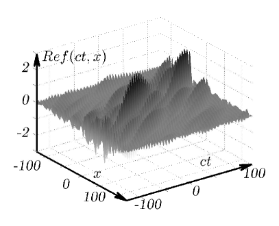
(a) The function $f(ct,x)$

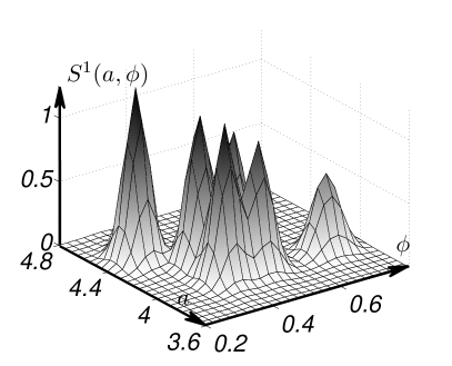
(b) The scale-rapidity diagram $S_{1}(a,\phi)$

Figure 6: An example of the scale-rapidity diagram.

We show that, analyzing the field in the plane $y=0$ by means of the wavelet transform, we can determine the parameters of the sources. The sources are far from the observation plane, and we do not calculate the wavelet transforms in domains ${\cal{D}}_{3,4}$, because the contribution of the components propagating along the surface are negligible.

We show that the wavelet transform enables us to find the frequencies and speeds of sources. We are not interested in the determination of the position of sources; for this reason we introduce a function $S(a,\phi)$, which reads

$$S_{1}(a,\phi)=\frac{1}{{a^{3}}}{\int\limits_{\mathbb{R}^{2}}d^{2}\boldsymbol{b}\ |F_{1}(\mu)|^{2}},\quad\mu=\{\boldsymbol{b},a,\phi\}.$$ (41)

Such a function, corresponding to the field in Fig.6a, as a function of the scaling $a$ and the rapidity $\phi$ is given in Fig.6b. The scale-rapidity diagram shown is calculated with the following wavelet parameters: $\varkappa=4,\sigma_{\parallel}=2\sqrt{55}\approx 15,\sigma_{\perp}=8$, the calculation mesh is from $-128$ to $128$ with step $0.5$ in both $x$ and $ct$. We see six maxima in this figure, which correspond to each group of sources. The position of the maximum $a,\phi$ contains information about the frequency $\omega=1/a$ and the average rapidity $\phi$ of sources. (We recall that the speed $v$ is connected with $\phi$ by the relation $v/c=\tanh\phi.$) The domain of integration in the decomposition formula must contain values of the parameters $a$, $\phi$ such that $S$ is not small. If we are interested only in the investigation of sources of certain frequencies and rapidities, we need to take the corresponding domain of integration.

A more complicated situation where the sources are masked by noise are considered by us in [10]. It is shown therein that the contribution of a noise can be eliminated, because it is located at small scales on the scale-rapidity diagram. The parameters of sources are found.

Appendix A The reconstruction formula

We prove the Plancherel equality (14) for the affine Poincaré wavelet transform (12) to make the paper self-contained. For the sake of brevity, we assume that $f\equiv g$. With account of (15) the Plancherel equality reads

$${\int\limits_{\mathbb{R}}d\phi}{\int\limits_{0}^{\infty}\frac{da}{a^{3}}}{\int\limits_{\mathbb{R}^{2}}d^{2}\boldsymbol{b}}\ \left|F_{j}(\boldsymbol{b},a,\phi)\right|^{2}=C_{j}\int\limits_{\mathbb{R}^{2}}d^{2}\boldsymbol{\chi}\left|f_{j}(\boldsymbol{\chi})\right|^{2},$$ (42)

where $C_{j}$ is defined by relation (11).
Applying the Plancherel equality (13) to the inner integral with respect to $\boldsymbol{b}$ and taking into account the definition of $F_{j},$ we obtain

$${\int\limits_{\mathbb{R}^{2}}d^{2}\boldsymbol{b}}\ \left|F_{j}(\boldsymbol{b},a,\phi)\right|^{2}=\frac{a^{2}}{(2\pi)^{2}}\int\limits_{\mathbb{R}^{2}}d^{2}{\sigma}\left|\hat{f}(\sigma)\right|^{2}\,\left|\hat{\psi}_{j}(a\Lambda_{-\phi}\boldsymbol{\sigma})\right|^{2}.$$ (43)

Here we use the fact that $F_{j}$ is a convolution of two functions $f(\boldsymbol{\chi})$ and $\overline{\psi_{j\mu}}(-\boldsymbol{\chi})$. Then it is used that the Fourier transform of $\overline{\psi_{j\mu}}(-\boldsymbol{\chi})$ is $\overline{\widehat{\psi_{j\mu}}(\boldsymbol{\sigma})},$ which is calculated by the formula (9).

Substituting (43) in the left-hand side of (42) and interchanging the order of integration, we obtain

$${\int\limits_{\mathbb{R}}d\phi}{\int\limits_{0}^{\infty}\frac{da}{a^{3}}}{\int\limits_{\mathbb{R}^{2}}d^{2}\boldsymbol{b}}\ \left|F_{j}(\boldsymbol{b},a,\phi)\right|^{2}=\frac{1}{(2\pi)^{2}}\int\limits_{\mathbb{R}^{2}}d^{2}{\boldsymbol{\sigma}}\left|\hat{f}(\boldsymbol{\sigma})\right|^{2}\int\limits_{\mathbb{R}}d{\phi}\int\limits_{0}^{\infty}\frac{da}{a}\,\left|\hat{\psi}_{j}(a\Lambda_{-\phi}\boldsymbol{\sigma})\right|^{2}$$ (44)

The next step is an analysis of the inner integral on the right-hand side of (44) . For the sake of definiteness, we assume that $j=1$. We transform the variable of integration in the following way:

$$\boldsymbol{\sigma}^{\prime}=a\Lambda_{-\phi}\sigma=a\binom{k\cosh\phi+k_{x}\sinh\phi}{k\sinh\phi+k_{x}\cosh\phi}=a\binom{\rho\cosh(\phi+\phi_{0})}{\rho\sinh(\phi+\phi_{0})}=\rho^{\prime}\binom{\cosh\phi^{\prime}}{\sinh\phi^{\prime}}.$$ (45)

Here we use the notation: $k=\rho\cosh\phi_{0}$, $k_{x}=\rho\sinh\phi_{0}$, $\rho>0$. Instead of $a$ and $\phi$ we take new variables $\phi^{\prime}=\phi+\phi_{0}$ and $\rho^{\prime}=a\rho$, $\phi^{\prime}\in(-\infty,+\infty),$ $\rho^{\prime}\in(0,\infty).$ Then the vector variable $\boldsymbol{\sigma}^{\prime}$ is chosen instead of $\phi^{\prime},$ $\rho^{\prime}.$ It takes values in ${\cal D}_{1}.$ The inner integral for any fixed $\boldsymbol{\sigma}$ is transformed as follows:

$$\int\limits_{\mathbb{R}}d{\phi}\int\limits_{0}^{\infty}\frac{da}{a}\,\left|\hat{\psi}_{j}(a\Lambda_{-\phi}\boldsymbol{\sigma})\right|^{2}=\int\limits_{\mathbb{R}}d{\phi^{\prime}}\int\limits_{0}^{\infty}\frac{\rho^{\prime}d\rho^{\prime}}{\rho^{\prime 2}}\bigl{|}\hat{\psi}_{j}(\boldsymbol{\sigma}^{\prime})\bigr{|}^{2}$$ (46)

$$=\int\limits_{\mathbb{R}^{2}}d^{2}{\boldsymbol{\sigma}^{\prime}}\frac{\bigl{|}\hat{\psi}_{j}(\boldsymbol{\sigma^{\prime}})\bigr{|}^{2}}{k^{\prime 2}-k^{\prime 2}_{x}}\equiv C_{j},\quad\boldsymbol{\sigma}^{\prime}=\binom{k^{\prime}}{k^{\prime}_{x}}.$$ (47)

Formula (14) has a generalization, in which $f,g$ are any functions from $\mathbb{L}_{2}$ and the wavelet transforms of the functions $f$ and $g$ denoted by $F_{j}$ and $G_{j},$ respectively, are calculated with different mother wavelets, say $\zeta$ and $\psi,$ respectively. In this case, formula (14) is valid, but $C_{j}$ is calculated as follows:

$$C_{j}=\int\limits_{{\cal{D}}_{j}}d^{2}\boldsymbol{\sigma}\,\frac{\overline{\hat{\zeta}_{j}(\boldsymbol{\sigma})}\hat{\psi}_{j}(\boldsymbol{\sigma})}{|(\omega/c)^{2}-k^{2}_{x}|}<\infty.\,$$ (48)

The reconstruction formula (16) may be obtained from (14) formally if we choose as a function $g$ any sequence of functions that tends to the Dirac $\delta$ function. To pass to the limit under the sign of the integral in (14) , we must impose additional restrictions on the functions $f$ and $g.$

Appendix B Ellipse transformations

Assume that the packet (31) is negligible outside the ellipse, i.e. if $\alpha^{2}(x^{\prime})^{2}+\beta^{2}(y-ct^{\prime})^{2}\geq 1$ in the moving frame. In the stationary frame this ellipse is distorted as follows:

$$\alpha^{2}\cosh^{2}\phi(x-x_{0})^{2}+\beta^{2}((y-y_{0})-\sinh\phi(x-x_{0}))^{2}\geq 1$$ (49)

The solution is located in the ellipse which reads in the main axes

$$\lambda_{1}\tilde{x}^{2}+\lambda_{2}\tilde{y}^{2}\leq 1.$$ (50)

where $\lambda_{j},j=1,2$ are eigenvalues of the matrix of the quadratic form in the left-hand side of the inequality (49) which are as follows

$$\lambda_{1,2}=\frac{(\alpha^{2}+\beta^{2})\cosh^{2}\phi}{2}\pm\frac{1}{2}\sqrt{(\alpha^{2}+\beta^{2})^{2}\cosh^{4}\phi-4\alpha^{2}\beta^{2}\cosh^{2}\phi}).$$ (51)

The directions of main axes read

$$\boldsymbol{e_{1,2}}=\left(\begin{array}[]{c}\beta^{2}-\alpha^{2}\cosh^{2}\phi-\beta^{2}\sinh^{2}\phi\pm\sqrt{(\alpha^{2}+\beta^{2})^{2}\cosh^{4}\phi-4\alpha^{2}\beta^{2}\cosh^{2}\phi}\\ 2\beta^{2}\sinh\phi\end{array}\right)$$ (52)

The new coordinates $\tilde{x}$, $\tilde{y}$ are connected with old coordinates $x-x_{0},$ $y-y_{0}$ by the relation

$$\binom{\tilde{x}}{\tilde{y}}=U^{\top}\binom{x-x_{0}}{y-y_{0}},\quad U=\left(\frac{\boldsymbol{e}_{1}}{|\boldsymbol{e}_{1}|},\frac{\boldsymbol{e}_{2}}{|\boldsymbol{e}_{2}|}\right)$$ (53)

where the columns of the matrix $U$ are vectors $\boldsymbol{e_{j}},j=1,2.$

References

References

• [1] Antoine, J. - P. , Murenzi, Vandergheynst,R. P. & Ali, S. T. , 2004, Two-dimensional wavelets and their relatives, Cambridge, Cambridge University Press, UK
• [2] Klauder, J. R. & Streater, R. F., 1991, A wavelet transform for the Poincare group, J. Math. Phys., Vol. 32, pp. 1609–1611
• [3] Bohnke, G., 1991, Treillis d’ondelettes associés aux groupes de Lorentz, 1991, Annales de l’I.H.P. Physique théorique, Vol. 54, pp. 245-259
• [4] Kaiser, G., 1994, A Friendly Guide to Wavelets (Boston:Birkhäuser)
• [5] Perel, M.V. & Sidorenko, M.S., 2003, Wavelet Analysis in Solving the Cauchy Problem for the Wave Equation in Three-Dimensional Space In: Waves 2003, Ed G C Cohen, E Heikkola, P Jolly and P Neittaanmaki (Springer-Verlag), pp 794-798
• [6] Perel, M.V. & Sidorenko M.S., 2006, Wavelet analysis for the solution of the wave equation, In: Proc. of the Int. Conf. DAYS on DIFFRACTION 2006, Ed. I V Andronov (SPbU), pp 208-217
• [7] Perel, M.V. & Sidorenko, M.S., 2009, Wavelet-based integral representation for solutions of the wave equation, J. Phys. A: Math. Theor., Vol. 42, pp. 3752–63
• [8] Perel, M. & Sidorenko, M. & Gorodnitskiy E., 2010, Multiscale investigation of solutions of the wave equation, In: Integral Methods in Science and Engineering, Vol. 2 Computational Methods, Eds.Constanda, C.; Perez, M.E., A Birkhäuser book, pp. 291–300
• [9] Perel, M.V., 2009, Integral representation of solutions of the wave equation based on Poincaré wavelets, In: Proc. of the Int. Conf. DAYS on DIFFRACTION 2009, Ed. I. V. Andronov (SPbU), pp. 159-161
• [10] Gorodnitskiy, E.A. & Perel, M.V., 2011, The Poincaré wavelet transform: implementation and interpretation, In: Proc. of the Int. Conf. DAYS on DIFFRACTION 2011, Ed. I. V. Andronov (SPbU), pp 72-77
• [11] Kiselev, A. P., & Perel, M. V., 1999, Gaussian wave packets, Optics & Spectroscopy, Vol. 86(3), 357-359
• [12] Kiselev, A.P. & Perel, M.V., 2000, Highly localized solutions of the wave equation, J.Math.Phys., Vol. 41(4), pp. 1934–55
• [13] Perel, M. V. & Fialkovsky, I. V., 2003, Exponentially Localized Solutions to the Klein-Gordon Equation, Journal of Mathematical Sciences, Vol. 117(2), 3994-4000
• [14] Perel, M.V. & Sidorenko, M.S. 2007, New physical wavelet Gaussian wave packet , J. Phys. A: Math. Theor., Vol. 40, pp. 3441–61
• [15] Kiselev, A. P., 2007, Localized light waves: Paraxial and exact solutions of the wave equation (a review), Optics & Spectroscopy Vol. 102(4), 603-622,
• [16] Localized Waves, Eds. H. E. Hernández-Figueroa, M. Zamboni-Rached , E. Recami (Editor),2008, Wiley-Interscience, USA
• [17] Saari, P. and Reivelt, K., 2004, Generation and classification of localized waves by Lorentz transformations in Fourier space, Phys. Rev. E, Vol. 69, 036612