Periodic orbits in the restricted four–body problem
with two equal masses

Abstract

The restricted (equilateral) four-body problem consists of three bodies of masses $m_{1}$, $m_{2}$ and $m_{3}$ (called primaries) lying in a Lagrangian configuration of the three-body problem i.e., they remain fixed at the apices of an equilateral triangle in a rotating coordinate system. A massless fourth body moves under the Newtonian gravitation law due to the three primaries; as in the restricted three-body problem (R3BP), the fourth mass does not affect the motion of the three primaries. In this paper we explore symmetric periodic orbits of the restricted four-body problem (R4BP) for the case of two equal masses where they satisfy approximately the Routh’s critical value. We will classify them in nine families of periodic orbits. We offer an exhaustive study of each family and the stability of each of them.

2

Keywords: Periodic orbits, four–body problem, stability, characteristic curves, asymptotic orbits.

AMS Classification: 70F15, 70F16

1 Introduction

Few bodies problems have been studied for long time in celestial mechanics, either as simplified models of more complex planetary systems or as benchmark models where new mathematical theories can be tested. The three–body problem has been source of inspiration and study in Celestial Mechanics since Newton and Euler. In recent years it has been discovered multiple stellar systems such as double stars and triple systems. The restricted three body problem (R3BP) has demonstrated to be a good model of several systems in our solar system such as the Sun-Jupiter-Asteroid system, and with less accuracy the Sun-Earth-Moon system. In analogy with the R3BP, in this paper we study a restricted problem of four bodies consisting of three primaries moving in circular orbits keeping an equilateral triangle configuration and a massless particle moving under the gravitational attraction of the primaries. Here we focus on the study of families of periodic orbits. We refer to this as the restricted four body problem (R4BP). There exist some preliminary studies of this problem in different versions, Simó (1978), Leandro (2006), Pedersen (1944) and Baltagiannis & Papadakis (2011b) studied the equilibrium points and their stability of this problem. Other authors have studied the case where the primaries form a collinear configuration. At the time of writing this paper we became aware of the paper Baltagiannis & Papadakis (2011), where they performed a numerical study similar to ours for two cases depending on the masses of the primaries: (a) three equal masses and (b) two equal masses. It is the second case that our work is related to Baltagiannis & Papadakis (2011), although we use a slightly different value of the mass parameter. The reason is the same as the cited authors, of having the primaries moving in linearly stable circular orbits for a value of the mass parameter less but approximately equal to Routh’s critical value. By historical and theoretical aspects, we use the same letters used in the Copenhagen category of the R3BP to denote the families of periodic orbits, see Szebehely (1967). The families $g$, $f$, $a$, $m$, $r_{2}$, $g_{4}$, $g_{6}$ are similar to those families denoted by the same letter in the R3BP, i.e., the family of direct periodic orbits around the mass $m_{1}$ of this paper is denoted by the letter $g$ as it was done in the Copenhagen category for each family, but the families $j$ and $j_{2}$ are exclusive of this problem because they do not have similar families in the R3BP. Our results confirm and extend four families of periodic orbits found in Baltagiannis & Papadakis (2011), such families are $f_{5}$, $f_{7}$, $f_{2}$, $f_{3}$. These families correspond respectively to the first phases (defined in 3.1) of the families $a$, $j$, $f$, $g$ of this paper, however we present 5 new families of periodic orbits. We used systematically regularization of binary collisions of the infinitesimal with any of the primaries by a method similar to Birkhoff’s which permit us to continue some of the families beyond double collisions. In this way we can show that such continued families end up in a homoclinic connection. This last phenomenon can be dynamically explained by the so called blue sky catastrophe and a rigorous justification will appear elsewhere.

We recall that Routh’s criterion for linear stability states that

$$\frac{m_{1}m_{2}+m_{2}m_{3}+m_{3}m_{1}}{m_{1}+m_{2}+m_{3}}<\frac{1}{27}.$$

When the three masses are such that $m_{2}=m_{3}:=\mu$ and $m_{1}+m_{2}+m_{3}=1$, the inequality is satisfied in the interval $\mu\in[0,0.019063652805978857\ldots)$, so in our case we take the masses equal to $m_{2}=m_{3}=0.0190636$ and $m_{1}=0.9809364$.

2 Equations of Motion

Consider three point masses, called primaries, moving in circular periodic orbits around their center of mass under their mutual Newtonian gravitational attraction, forming an equilateral triangle configuration. A third massless particle moving in the same plane is acted upon the attraction of the primaries. The equations of motion of the massless particle referred to a synodic frame with the same origin, where the primaries remain fixed, are:

$$\bar{x}^{\prime\prime}-2n\bar{y}^{\prime}-n^{2}\bar{x} = -k^{2}\sum_{i=1}^{3}m_{i}\frac{(\bar{x}-\bar{x_{i}})}{\rho_{i}^{3}}$$

$$\bar{y}^{\prime\prime}+2n\bar{x}^{\prime}-n^{2}\bar{y} = -k^{2}\sum_{i=1}^{3}m_{i}\frac{(\bar{y}-\bar{y_{i}})}{\rho_{i}^{3}}$$ (1)

where $k^{2}$ is the gravitational constant, $n$ is the mean motion, $\rho_{i}^{2}=(\bar{x}-\bar{x}_{i})^{2}+(\bar{y}-\bar{y}_{i})^{2}$ is the distance of the massless particle to the primaries, $\bar{x}_{i}$, $\bar{y}_{i}$ are the vertices of equilateral triangle formed by the primaries, and (^′) denotes derivative with respect to time $t^{*}$. We choose the orientation of the triangle of masses such that $m_{1}$ lies along the positive $x$–axis and $m_{2}$, $m_{3}$ are located symmetrically with respect to the same axis, see Figure 1.

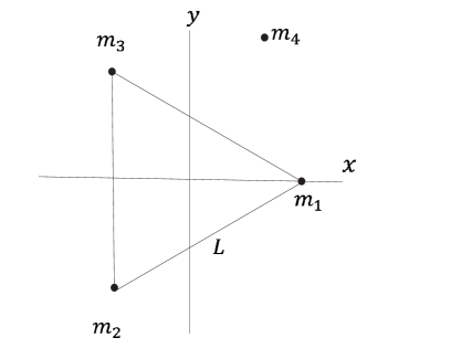
Fig. 1 : The restricted four-body problem in a synodic system

The equations of motion can be recast in dimensionless form as follows: Let $L$ denote the length of triangle formed by the primaries, $x=\bar{x}/L$, $y=\bar{y}/L$, $x_{i}=\bar{x}_{i}/L$, $y_{i}=\bar{y}_{i}/L$, for $i=1,2,3$; $M=m_{1}+m_{2}+m_{3}$ the total mass, and $t=nt^{*}$. Then the equations (1) become

$$\ddot{x}-2\dot{y}-x = -\sum_{i=1}^{3}\mu_{i}\frac{(x-x_{i})}{r_{i}^{3}}$$

$$\ddot{y}+2\dot{x}-y = -\sum_{i=1}^{3}\mu_{i}\frac{(y-y_{i})}{r_{i}^{3}}$$ (2)

where we have used Kepler’s third law: $k^{2}M=n^{2}L^{3}$, ($\dot{}$) represents derivatives with respect to the dimensionless time $t$ and $r_{i}^{2}=(x-x_{i})^{2}+(y-y_{i})^{2}$.

The system (2) will be defined if we know the vertices of triangle for each value of the masses. In this paper we suppose $\mu:=m_{2}=m_{3}$ then $\mu_{1}=1-2\mu$. It is not difficult to show that the vertices of triangle are given by $x_{1}=\sqrt{3}\mu$, $y_{1}=0$, $x_{2}=-\frac{\sqrt{3}(1-2\mu)}{2}$, $y_{2}=-\frac{1}{2}$, $x_{3}=-\frac{\sqrt{3}(1-2\mu)}{2}$, $y_{3}=\frac{1}{2}$. The system (2) can be written succinctly as

$$\ddot{x}-2\dot{y} = \Omega_{x}$$ (3)

$$\ddot{y}+2\dot{x} = \Omega_{y}$$ (4)

where

$$\Omega(x,y,\mu):=\frac{1}{2}(x^{2}+y^{2})+\sum_{i=1}^{3}\frac{\mu_{i}}{r_{i}}$$

is the effective potential function.

There are three limiting cases:

1. If $\mu=0$, we obtain the rotating Kepler’s problem, with $m_{1}=1$ at the origin of coordinates.

2. If $\mu=1/2$, we obtain the circular restricted three body problem, with two equal masses $m_{2}=m_{3}=1/2$.

3. If $\mu=1/3$, we obtain the symmetric case with three masses equal to $1/3$.

It will be useful to write the system (3) using complex notation. Let $z=x+\textit{i}y$, then

$$\ddot{z}+2\textit{i}\dot{z}=2\frac{\partial\Omega}{\partial\bar{z}}$$ (5)

with

$$\Omega(z,\bar{z},\mu)=\frac{1}{2}|z|^{2}+U(z,\bar{z},\mu)$$

where the gravitational potential is

$$U(z,\bar{z},\mu)=\sum_{i=1}^{3}\frac{\mu_{i}}{|z-z_{i}|}$$

and $r_{i}=|z-z_{i}|$, $i=1,2,3$ are the distances to the primaries. System (5) has the Jacobian first integral

$$2\Omega(z,\bar{z},\mu)-|\dot{z}|^{2}=C.$$

If we define $P=p_{x}+\textit{i}p_{y}$, the conjugate momenta of $z$, then system (3) can be recast as a Hamiltonian system with Hamiltonian

$$H = \frac{1}{2}|P|^{2}+Im(z\overline{P})-U(z,\bar{z},\mu)$$ (6)

$$= \frac{1}{2}(p^{2}_{x}+p^{2}_{y})+(yp_{x}-xp_{y})-U(x,y,\mu).$$

The relationship with the Jacobian integral is $H=-C/2$. The phase space of (6) is defined as

$$\Delta=\{(z,P)\in\mathbb{C}\times\mathbb{C}|z\neq z_{i},i=1,2,3\},$$

with collisions occurring at $z=z_{i}$, $i=1,2,3$.

There exist five equilibrium points for all values of the masses of the primaries in the R3BP; in the R4BP, the number of equilibrium points depends on the particular values of the masses. For the value of the mass parameter we are using throughout this paper of $\mu=0.0190636$, the Hill’s regions are shown in Figure 2. For large values of $C$ the Hill’s regions consist of small disks around the primaries together with an unbounded component having as boundary a closed curve around the primaries. As the Jacobian constant decreases, the evolution of the Hill’s region is shown in Figure 2. The smaller value of $C$ is just above the critical value where the Hill’s region is the whole plain minus the positions of the primaries.

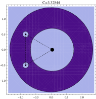
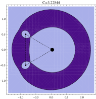
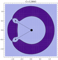
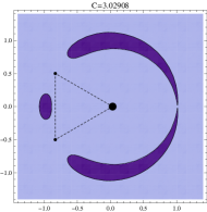
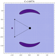
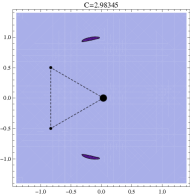
Fig. 2 : Hill’s regions for a large value of the Jacobian constant (top-left). Hill’s regions for critical values of the Jacobian constant (top-right and second row). The Hill’s regions of the last row correspond to a slightly larger value than the critical one for illustrations purposes.

A complete discussion of the equilibrium points and bifurcations can be found in Delgado & Álvarez–Ramirez (2003), Meyer (1987), Leandro (2006), Baltagiannis & Papadakis (2011b), Simó (1978). In our particular problem we have 2 collinear and 6 non-collinear equilibrium points. We use the notation shown in Figure 3 for the eight critical points. All of them are unstable except the non-collinear $L_{7}$ and $L_{8}$.

Fig. 3 : The eight equilibrium points (green) for two equal masses.

3 Symmetric periodic orbits

In what follows we consider symmetric periodic orbits, i,e., periodic orbits symmetric with respect to the synodical $x$-axis, namely orbits which are invariant under the symmetry $(z,t)\rightarrow(\bar{z},-t)$. Thus a symmetric periodic orbit is defined by two successive perpendicular crossings with the $x$-axis. We use as staring point of the continuation either nearly Keplerian circular orbits for large values of the Jacobian constant or small Liapunov’s orbits emerging form $L_{1}$. It was shown in Leandro (2006) that the equilibrium point $L_{1}$ is unstable with eigenvalues $\pm\textit{i}\omega$, $\pm\lambda$ where $\omega$ and $\lambda$ are real numbers, so we can use the Liapunov’s Center Theorem to find periodic orbits around the equilibrium point $L_{1}$ and continue them.

In the R3BP the equilibrium points $L_{4}$ and $L_{5}$ are limits of families of periodic orbits of the family $g$ of the Copenhagen category. This phenomenon is known as the “blue sky catastrophe” termination principle. In the papers by Buffoni (1999), Meyer & McSwiggen (2002) and Simó (1978) a complete discussion of this principle in the R3BP is given. We state the theorem behind this phenomena as stated in Henrard (1973):

Theorem 1

Let us consider a non-degenerate homoclinic orbit to an equilibrium with eigenvalues $\pm\alpha\pm i\omega$ with $\alpha$ and $\omega$ reals and strictly positive, of a real analytic Hamiltonian system with two degrees of freedom. Close to this orbit there exists an analytical family of periodic orbits with the following properties

1. The family can be parametrized by a parameter $\epsilon$ in the interval $0<\epsilon<\delta$ with $\delta$ small enough. Let us write it as $x(\epsilon,t)=x(\epsilon,t+T(\epsilon))$.

2. For $\epsilon=0$ we have the homoclinic orbit.

3. The period $T(\epsilon)$ increases without bound when $\epsilon$ goes to zero.

4. The characteristic exponents of the family change from the stable type to unstable type an vice-versa infinitely many times as $\epsilon$ goes to zero.

In a future work we will discuss the theoretical aspects of this termination principle in the R4BP.

In the following section we will classify a large number of periodic orbits in sets called families. We will take the Henon’s definition for a family of periodic orbits to make such classification (see Hénon (1997)):

Definition 1

A family of periodic orbits is a set of symmetric periodic orbits for which the initial parameter $x_{0}=x(0)$ and the period in family can be considered as two continuous functions of one single parameter $\alpha$.

In general we will consider the Strömgren’s termination principle to decide when a family ends.

Definition 2

Suppose we have obtained a finite section of a family of periodic orbits in an interval of the parameter $[\alpha_{1},\alpha_{2}]$ for which the family is followed and we want to extend it, then

1. The family remains in itself, i.e., the characteristic curve is a closed curve. We call this family a closed family.

2. For $\alpha\leq\alpha_{1}$ and $\alpha\geq\alpha_{2}$ the family has a natural termination for which one of the following amounts grow without limit

   • The dimension $D$ of the orbit, defined as the maximum distance to the origin.

   • The parameter $\alpha$.

   • The period of the orbit.

The second case is called an open family.

Note that the principle of termination of a family of periodic orbits mentioned in 1 is a particular case of the above definition because the period of the orbit increases without bound.

3.1 The search for periodic orbits

The periodic orbits were calculated in double precision with a multi-step Adams-Bashforth integrator of variable order for more accuracy. New transformations were needed to regularize different kind of collisions appearing in the families of periodic orbits of this problem. The families have been identified by letters as in the Copenhagen category with or without subscripts, the subscripts meaning the number of loops of the orbit around the primary under consideration. We use the classic $(x,C)$ plane of characteristic curves to represent the families of periodic orbits, in addition we use the $(a,C)$ plane to show the evolution of the stability of the families, here $a$ denotes the stability index (see Hénon (1965b) for details), we have stability in the linear sense when $|a|<1$ and instability in other case.

The families have been separated in phases as in the R3BP (see Szebehely (1967)), the colors in the characteristic curves of the nine families represent the different phases (and orbits near to collision) of each family, representative orbits are shown to illustrate each phase. Some orbits shown by Broucke (1968) and Baltagiannis & Papadakis (2011) can be compared with ours.

4 Classification of families of periodic orbits

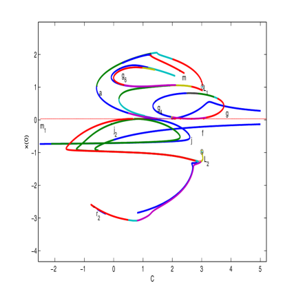
Fig. 4 : The characteristic curves of nine families of periodic orbits for the restricted four-body problem with two equal masses.

4.1 The family $g$ of direct periodic orbits around $m_{1}$

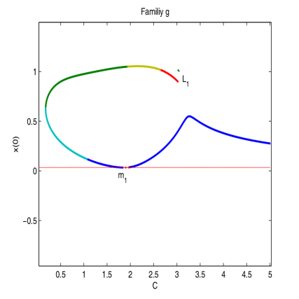
Fig. 5 : Characteristic curve of family $g$.

The first phase of this family stars with infinitesimal direct circular periodic orbits around $m_{1}$, the size of the orbits increases as the value of Jacobi constant $C$ decreases until a collision orbit is reached, the first phase of this family was established and studied in Baltagiannis & Papadakis (2011) for a little smaller value of $\mu$. Second phase starts with the retrograde orbit following the collision orbit which forms two loops as shown in Figure  17. The inside loops now increase their size and the outside loops shrink as the value of $C$ deceases, both sets of loops become indistinguishable at the $fold$ point when $C\approx 0.1797$. After this point the third phase starts, now the role of the loops is interchanged i,e., the inside loops shrinks and the outside loops expand as the value of $C$ increases.

Following the evolution of this phase we found that an orbit of collision with $m_{1}$ appears and the inside loops disappear, this is the beginning of fourth phase where the middle part of the orbits increases its size as the Jacobi constant increases, the termination of this phase (and of the whole family) are asymptotic orbits to $L_{2}$ ($L_{3}$ in Baltagiannis & Papadakis (2011)). More precisely, the value of $C$ oscillates in a small neighbourhood around the value of the Jacobi constant of the equilibrium point $L_{2}$ and the period tends to infinity as is predicted in theorem 1 similar to the Copenhagen category of R3BP.

4.2 The family $f$ of retrograde orbits around $m_{1}$

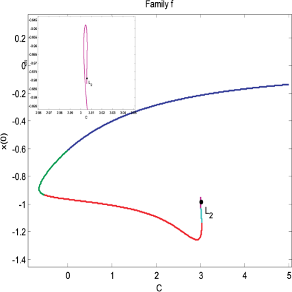
Fig. 6 : Characteristic curve of family $f$, zoomed area indicates the end of family at the equilibrium point $L_{2}$.

The first phase of this family starts with infinitesimal retrograde circular periodic orbits around $m_{1}$, as in family $g$ the size of the orbits increase as the value of $C$ decreases monotonically until a $fold$ point is reached, this happens at $C\approx-0.6379$. This is the beginning of second phase, the periodic orbits still continue increasing their size but now these orbits tend to collision with the primaries $m_{2}$ and $m_{3}$, however this collision is never reached because the periodic orbits become asymptotic to $L_{2}$, as in family $g$. See Figures  6, 18.

4.3 The family $a$ of retrograde orbits around $L_{1}$

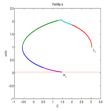
Fig. 7 : Characteristic curve of family $a$.

The beginning of this family is provided by the Liapunov’s center theorem, therefore in this family we continue retrograde periodic orbits around the equilibrium point $L_{1}$ ($L_{2}$ in Baltagiannis & Papadakis (2011)) for values of the Jacobi constant less than $C_{1}$. As the Jacobi constant decreases monotonically, the periodic orbits increase their size until a collision orbit with $m_{1}$ is reached; this is the end of first phase. While the value of $C$ continues decreasing, a second loop appears in the orbits, this loop increases its size along this second phase until a new $fold$ point is reached when $C\approx-0.5846$. At this point the inner and outer loops become indistinguishable as in the previous families, after this fold point, both loops are interchanged and the new inside loop shrinks as the value of $C$ increases until a collision orbit with $m_{1}$ finishes the third phase, see Figures  7, 19.

4.4 The family $g_{4}$

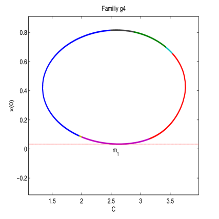
Fig. 8 : Characteristic curve of the closed family $g_{4}$.

This family is the first example in this paper of a closed family of periodic orbits, see Figures  8, 20. The first phase of this family is composed of periodic orbits forming four loops around $m_{1}$, following the evolution of first phase we found that as $C$ decreases the four loops shrink until they become indistinguishable i,e; a $fold$ point is reached at $C\approx 1.3381$, the second phase starts when these loops separate each other, as $C$ increases the periodic orbits tend to collision with $m_{1}$ i,e; the intersections between the loops tend to $m_{1}$. After this collision, the third phase starts. The periodic orbits change multiplicity because four inside loops around $m_{1}$ appear together with four outside loops. As the value of $C$ increases, the inside loops increase their size while the outside loops shrink at same time until they disappear. This is the end of third phase.

Fourth phase begins when the loops around $m_{1}$ increase their size as $C$ continues increasing monotonically. These loops become indistinguishable at the value $C\approx 3.7581$ and a new $fold$ point is reached. After this $fold$ point the fifth phase begins, as expected inside and outside loops interchange and the peak of the outside loops become non-smooth i,e; no more orthogonal intersections with $x$-axis exist, this is the end of fifth phase. As $C$ decreases the loops of the orbits shrink to collision with $m_{1}$ and the sixth phase ends. We observe that the first phase of this family starts after this collision, therefore the family is closed.

4.5 The family $g_{6}$

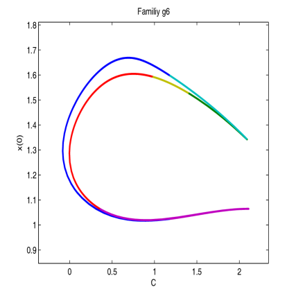
Fig. 9 : Characteristic curve of the closed family $g_{6}$.

This family is another example of a closed family of periodic orbits. The behavior of its orbits is more complicated than that of previous families see Figure  9, 21. We have named $g_{6}$ this family because there exist a section of this family where the orbits form 6 loops around the primary $m_{1}$ but following the evolution of this family, we find that the orbits show a complicated behavior, therefore is not clear at all how to classify in phases this family, for simplicity we use the term “first” phase to the outer section of the characteristic curve between the return points in Figure  9, and second phase to the inner section between the return points. In each case we show representative orbits in Figure  21.

4.6 The family $m$ of retrograde orbits around $m_{1}$, $m_{2}$ and $m_{3}$

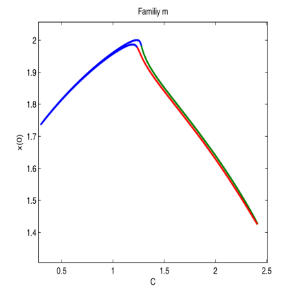
Fig. 10 : Characteristic curve of the closed family $m$.

Family $m$ consists of retrograde periodic orbits around the three primaries but these orbits do not surround the primaries simultaneously i,e., they form three loops, each loops surrounds one primary as can be seen in the Figure  (22). The characteristic curve of the family is shown in Figure  10 The three loops increase and decrease their size while the family is followed; however collision with the primaries never is reached although the orbits are close to collision when the loops decrease their size. This behavior is cyclic because the family is closed.

4.7 The family $j$ of retrograde periodic orbits around $m_{2}$ and $m_{3}$

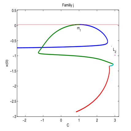
Fig. 11 : Characteristic curve of the family $j$.

The first phase of this family by one side tends to collision with the primaries $m_{2}$ and $m_{3}$, such collisions are reached for great values (negatives) of the Jacobi constant, see Figures  11, 23. As $C$ increases, the orbits increase their size around $m_{2}$ and $m_{3}$, the orthogonal intersection to the right of both primaries $m_{2}$ and $m_{3}$ tends to the primary $m_{1}$ and a collision orbit appears, this is the end of the first phase. After this collision an inner loop appears as expected and the orbits become direct around $m_{1}$, this is the second phase, the inside and the outside loops increase their size and the orbits tend to collision with both primaries $m_{2}$ and $m_{3}$ until this collision happens. The third phase starts after this collision, two loops around $m_{2}$ and $m_{3}$ respectively appear in the orbits and as $C$ decreases these loops these loops increase around the primaries, the behavior of the orbits complicate while the family is followed.

Finally a new collision orbit with $m_{1}$ appears. We have decided to terminate the family at this point, the complicated behavior of the orbits and the long time of integration of the regularized equations forced us to stop the continuation at this point.

4.8 The family $r_{2}$ of asymptotic orbits to $L_{2}$

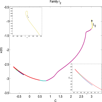
Fig. 12 : Characteristic curve of family $r_{2}$, zoomed areas indicate the end of family at the equilibrium point $L_{2}$ and a return point of the family.

This family of periodic orbits has been named $r_{2}$ in analogy with the family $r$ of the Copenhagen category, the subscript indicates that the family is asymptotic to $L_{2}$ see Figures  12, 24. The first phase of this family is composed by asymptotic periodic orbits to the equilibrium point $L_{2}$, these orbits form two loops surrounding the primaries $m_{2}$ and $m_{3}$ but while the periodic orbits go away from $L_{2}$ these loops shrink, therefore we have orbits close to collision now, however such collision never is reached. When the value of $C$ begins to decrease monotonically these loops increase its size and therefore the period of the orbits increase, it is interesting to note that the orbits become symmetric respect to $y$-axis (see Figure  24) however this symmetry disappears as $C$ continues decreasing, a collision orbits with $m_{1}$ terminates the first phase.

As expected, a new loop around $m_{1}$ appears in the orbits, here the second phase starts, following the evolution of the family we can see that the resulting loops of the collision increases its size as $C$ decreases monotonically and the orbits tend to collision with the primaries $m_{2}$ and $m_{3}$ . At $C\approx-0.7726$ we find a return point. We must emphasize that such collision is not reached although the mentioned loop continues increasing its size and therefore the orbits increase their period. This behavior continues as $C$ increases monotonically. As in family $j$ the long period of the orbits (long time of integration of the equations is needed) and the high instability of the orbits did not allow us to establish the end of this phase and therefore of the whole family.

4.9 The family $j_{2}$ of retrograde periodic orbits around $m_{2}$ and $m_{3}$

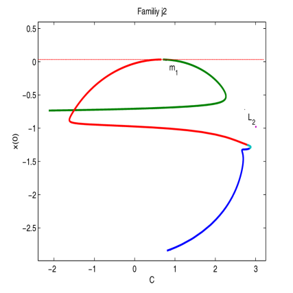
Fig. 13 : Characteristic curve of the family $j_{2}$, note it is very similar to the one of the family j.

This last family named $j_{2}$ contains retrograde periodic orbits around $m_{2}$ and $m_{3}$ as in family $j$ but this time the orbits have an extra loop around $m_{2}$ and $m_{3}$ and this loop surrounds the primary $m_{1}$ too (see Figures  13, 25). The evolution of this family is very similar to the evolution of family $j$, in fact, its characteristic curve has the same form that the one of family $j$. We show representative orbits of each phase in Figure  25.

5 Stability of families and critical points

5.1 Critical points

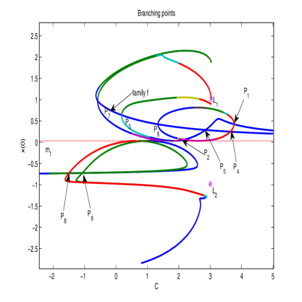
Fig. 14 : Branching points between the families of periodic orbits

As can be seen in Hénon (1997), when we follow families of periodic orbits it can be found some especial points in such families called critical points such as fold points and branching points, the last point is where two characteristic curves intersect, in 5.2 we will see that these points are in relation with stability changes, this facts do not ocurr by casuality, such phenomena was studied by example in Hénon (1965b). We must say that some families of periodic orbits were found through these points, in Figure  14 we show the branching points found in this study.

1. Family $g$ has 3 branching points; first one $P_{1}$ at $C\approx 3.7581$ with family $g_{4}$, second one $P_{2}$ at $C\approx 2.1662$ with family $g_{4}$ again, third one $P_{3}$ at $C\approx 0.1797$ with family $f$. This last branching point happens at a fold point.

2. Family $f$ has 5 branching points, first one $P_{4}$ at $C\approx 3.6364$ with family $g_{4}$, second one $P_{5}$ at $C\approx 2.8481$ with family $g$, third one $P_{6}$ at $C\approx 1.3381$ with family $g_{4}$, fourth one $P_{3}$ with family $g$ already mentioned, fifth one $P_{7}$ at $C\approx-0.5846$ with family $a$ ($fold$ point of family $a$)

3. Families $j$ and $j_{2}$ intersect at two points, first one $P_{8}$ at $C\approx-1.5015$ and second one $P_{9}$ at $C\approx-1.073$.

5.2 Stability of families

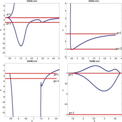
Fig. 15 : Stability curve of family $g$ (up left), stability curve of family $f$ (up right), stability curve of family $a$ (down left), stability curve of family $g_{4}$ (down right).

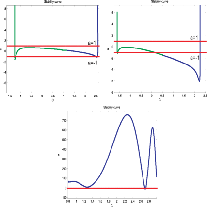
Fig. 16 : Stability curve of family $j$ (up left), stability curve of family $j_{2}$ (up right), part of the end of the stability curve of family $r_{2}$ (center).

In family $g$ we see that the first and second phase contain stable periodic orbits, at the end of second phase in the critical ($fold$) point we have that $|a|=1$ as expected, after this critical point all orbits become unstable, at the end of this family we observe strong oscillations of the sign of $a$ and therefore between the stable and unstable areas as is predicted by the “blue sky catastrophe” termination. In family $f$ we have that the first phase of this family posses stable orbits as is shown in the Figure  15, at the $fold$ point we have $|a|=1$ again, after this point all orbits are unstable until the termination of family is reached and as in family $g$ strong oscillations between stable and unstable orbits are observed.

In family $a$ almost all orbits are unstable but we have 3 small regions where the orbits are stable, one of them is in the first phase, the second one is at the end of second phase; in the $fold$ point we have of course $|a|=1$. After this point the stability index starts to decrease and therefore we find a stability region at the beginning of third phase. The family $g_{4}$ is a closed family, a “half” of its orbits are stable and a “half” are unstable, this affirmation can be seen in Figure  15, at the two $fold$ points we have $|a|=1$ and between these two points the stability changes occur.

In family $g_{6}$ almost all orbits are unstable, only a very little region around the two $fold$ points has stable orbits. Family $m$ presents a similar behavior as in family $g_{6}$. Orbits in family $r_{2}$ are strongly unstable except at the termination of family where oscillatory behavior between areas of stability and instability is observed. In the family $j$ we found a stability region between the values $C\approx-1.27$ and $C\approx 2.59$, see Figure  16 in this interval we have 3 critical points on the characteristic curve, and this can be seen on the stability curve where we have values for which $|a|=1$. For the family $j_{2}$ we have its stability curve behaves similar to the one of the family $j$, see Figure  16.

6 Examples of periodic orbits

In Figures  17, 25 we show representative orbits of each phase of the nine found families of periodic orbits. Each row in the following figures represent a phase of the family, the first row represent the first phase of the family, second row represent the second phase etc.

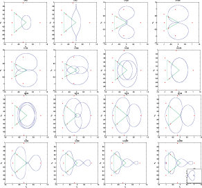
Fig. 17 : Phases of family g.

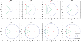
Fig. 18 : Phases of family f.

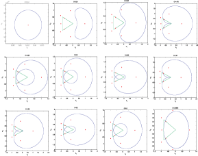
Fig. 19 : Phases of family a.

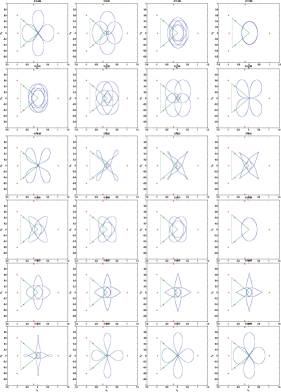
Fig. 20 : Phases of family $g_{4}$.

Fig. 21 : Phases of family $g_{6}$.

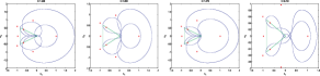
Fig. 22 : Phases of family m.

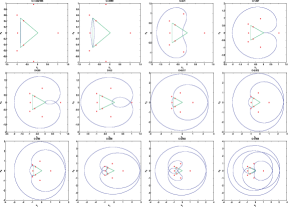
Fig. 23 : Phases of family $j$.

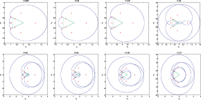
Fig. 24 : Phases of family $r_{2}$.

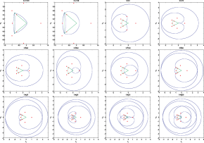
Fig. 25 : Phases of family $j_{2}$.

7 Conclusions and remarks

In this work we extend the previous study of Baltagiannis & Papadakis (2011) and we include $5$ new families of periodic orbits. We performed the numerical continuation beyond different collisions with the primaries and show how some of them end up in a homoclinic orbit as predicted by the “blue sky catastrophe” termination principle. In the former section we show representative orbits for each phase of the families, the orbits are mainly retrograde but there are families consisting of direct periodic orbits. We have also studied the stability of each family of periodic orbits and we show the characteristic curve of seven families where a considerable number of stable periodic orbits were found. Our main results can be summarized as follows:

1. The families $g$, $f$, $a$, $g_{4}$, $j$, $j_{2}$, and $r_{2}$ present a large number of stable periodic orbits, all the orbits in the families $g_{6}$ and $m$ are unstable except in very small regions.

2. The families $g$, $f$ and $r_{2}$ are asymptotic to the equilibrium point $L_{2}$, i,e; they end according to the “Blue Sky Catastrophe” termination principle.

3. The families $g_{4}$, $g_{6}$ and $m$ are closed families.

4. The families $g$, $f$, $a$, $g_{4}$, $j$, and $j_{2}$ present Branching points between their characteristic curves.

5. Almost all the families consist of retrograde periodic orbits, except families $g$, $g_{4}$ where have direct ones.

Acknowledgements Author Burgos–García has been supported by a CONACYT fellowship of doctoral studies.

References

- Álvarez-Ramirez & Vidal, C. (2009) Álvarez-Ramirez, M., Vidal, C.: Dynamical aspects of an equilateral restricted four-body problem. Math. Probl. Eng. (2009). doi:10.1155/2009/181360
- Baltagiannis & Papadakis (2011) Baltagiannis, A.N., Papadakis, K.E.: Families of periodic orbits in the restricted four-body problem. Astrophys. Space Sci. 336, 357–367 (2011)
- Baltagiannis & Papadakis (2011b) Baltagiannis, A.N., Papadakis, K.E.: Equilibrium points and their stability in the restricted four-body problem. Int. J. Bifurc. Chaos. 21, 2179–2193 (2011)
- Broucke (1968) Broucke, R. A.: Periodic orbits in the restricted three–body problem with earth-moon masses. Technical Report, JPL. (1968)
- Buffoni (1999) Buffoni, B.: Shooting methods and topological transversality. Proc. Roy. Soc. Edinburgh. Sec. A. 129, 1137–1155 (1999)
- Ceccaroni & Biggs (2010) Ceccaroni, M., Biggs, J.: Extension of low-thrust propulsion to the autonomous coplanar circular restricted four body problem with application to future Trojan Asteroid missions. In: 61st Int. Astro. Congress IAC 2010 Prague, Czech Republic (2010)
- Delgado & Álvarez–Ramirez (2003) Delgado, J., Álvarez–Ramirez, M.: Central Configurations of the symmetric restricted four-body problem. Cel. Mech. and Dynam. Astr. 87, 371–381 (2003)
- Govaerts (2000) Govaerts, W.: Numerical methods for bifurcations of dynamical equilibria. SIAM. USA. (2000)
- Hénon (1965) Hénon, M.: Exploration numérique du probléme restreint I. Masses égales, Orbites périodiques. Ann. Astrophysics 28, 499–511 (1965)
- Hénon (1965b) Hénon, M.: Exploration numérique du probléme restreint II. Masses égales, stabilité des orbites périodiques. Ann. Astrophysics 28, 992–1007 (1965)
- Hénon (1997) Hénon, M.: Generating families in the restricted three body problem. Springer Verlag (1997)
- Henrard (1973) Henrard, J.: Proof of a conjeture of E. Strömgren. Cel. Mech.7, 449–457 (1973)
- Kusnetzov (2004) Kusnetzov, Yu. A.: Elements of applied bifurcation theory. Springer Verlag (2004)
- Leandro (2006) Leandro, E. S. G.: On the central configurations of the planar restricted four–body problem. J. Differential Equations 226, 323–351 (2006)
- Meyer (1987) Meyer, K.: Bifurcation of a central configuration. Cel. Mech. 40(3–4), 273-282 (1987)
- Meyer (2009) Meyer, K.: Introduction to Hamiltonian Dynamical Systems and the N–body problem. Springer Verlag (2009)
- Meyer & McSwiggen (2002) Meyer, K., McSwiggen, P.D.: The evolution of invariant manifolds in Hamiltonian-Hopf bifurcations. J. Differential Equations 189, 538–555 (2002)
- Pedersen (1944) Pedersen, P. : Librationspunkte im restringierten vierkoerperproblem. Dan. Mat. Fys. Medd. 1–80 (1944)
- Schwarz & Sülli (2009) Schwarz, R., Sülli, Á., Dvorac, R., Pilat-Lohinger, E.: Stability of Trojan planets in multi-planetary systems. Cel. Mech. Dyn. Astron. 69-84 (2009)
- Simó (1978) Simó, C.: Relative equilibrium solutions in the four body problem. Cel. Mech. 165-184 (1978)
- Szebehely (1967) Szebehely, V.: Theory of orbits. Academic Press, New York (1967)