Copolymer with pinning:
variational characterization of the phase diagram
Abstract
This paper studies a polymer chain in the vicinity of a linear interface separating two immiscible solvents. The polymer consists of random monomer types, while the interface carries random charges. Both the monomer types and the charges are given by i.i.d. sequences of random variables. The configurations of the polymer are directed paths that can make i.i.d. excursions of finite length above and below the interface. The Hamiltonian has two parts: a monomer-solvent interaction (“copolymer”) and a monomer-interface interaction (“pinning”). The quenched and the annealed version of the model each undergo a transition from a localized phase (where the polymer stays close to the interface) to a delocalized phase (where the polymer wanders away from the interface). We exploit the approach developed in [5] and [3] to derive variational formulas for the quenched and the annealed free energy per monomer. These variational formulas are analyzed to obtain detailed information on the critical curves separating the two phases and on the typical behavior of the polymer in each of the two phases. Our main results settle a number of open questions.
AMS 2000 subject classifications. 60F10, 60K37, 82B27.
Key words and phrases. Copolymer with pinning, localization vs. delocalization,
critical curve, large deviation principle, variational formulas.
Acknowledgment. FdH was supported by ERC Advanced Grant VARIS 267356, AO by NWO-grant 613.000.913.
1 Introduction and main results
1.1 The model
1. Polymer configuration. The polymer is modeled by a directed path drawn from the set
| (1.1) |
of directed paths in that start at the origin and visit the interface when switching from the lower halfplane to the upper halfplane, and vice versa. Let be the path measure on under which the excursions away from the interface are i.i.d., lie above or below the interface with equal probability, and have a length distribution on with a polynomial tail:
| (1.2) |
The support of is assumed to satisfy the following non-sparsity condition
| (1.3) |
Denote by the restriction of to -step paths that end at the interface.
2. Disorder. Let and be subsets of . The edges of the paths in are labeled by an i.i.d. sequence of -valued random variables with common law , modeling the random monomer types. The sites at the interface are labeled by an i.i.d. sequence of -valued random variables with common law , modeling the random charges. In the sequel we abbreviate with and assume that and are independent. We further assume, without loss of generality, that both and have zero mean, unit variance, and satisfy
| (1.4) |
We write for the law of , and and for the laws of and .
3. Path measure. Given and , the quenched copolymer with pinning is the path measure given by
| (1.5) |
where and are parameters, is the normalizing partition sum, and
| (1.6) |
is the interaction Hamiltonian, where and (the -th edge is below or above the interface).
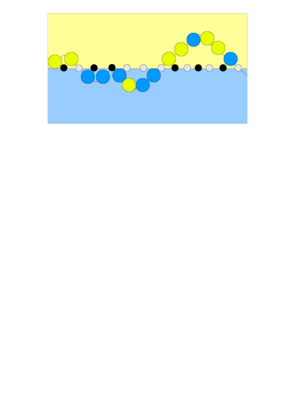
Key example: The choice corresponds to the situation where the upper halfplane consists of oil, the lower halfplane consists of water, the monomer types are either hydrophobic () or hydrophilic (), and the charges are either positive () or negative (); see Fig. 1. In (1.6), and are the strengths of the monomer-solvent and monomer-interface interactions, while and are the biases of these interactions. If is the law of the directed simple random walk on , then (1.2) holds with .
In the literature, the model without the monomer-interface interaction () is called the copolymer model, while the model without the monomer-solvent interaction () is called the pinning model (see Giacomin [11] and den Hollander [12] for an overview). The model with both interactions is referred to as the copolymer with pinning model. In the sequel, if is a quantity associated with the combined model, then and denote the analogous quantities in the copolymer model, respectively, the pinning model.
1.2 Quenched excess free energy and critical curve
The quenched free energy per monomer
| (1.7) |
exists -a.s. and in -mean (see e.g. Giacomin [7]). By restricting the partition sum to paths that stay above the interface up to time , we obtain, using the law of large numbers for , that . The quenched excess free energy per monomer
| (1.8) |
corresponds to the Hamiltonian
| (1.9) |
and has two phases
| (1.10) | ||||
called the quenched localized phase (where the strategy of staying close to the interface is optimal) and the quenched delocalized phase (where the strategy of wandering away from the interface is optimal). The map is non-increasing and convex for every and . Hence, and are separated by a single curve
| (1.11) |
called the quenched critical curve.
In the sequel we write , , , for the analogous quantities in the copolymer model (), and , , , for the analogous quantities in the pinning model ().
1.3 Annealed excess free energy and critical curve
The annealed excess free energy per monomer is given by
| (1.12) |
where is the expectation w.r.t. the joint disorder distribution . This also has two phases,
| (1.13) | ||||
called the annealed localized phase and the annealed delocalized phase, respectively. The two phases are separated by the annealed critical curve
| (1.14) |
Let . We will show in Section 3.2 that
| (1.15) | ||||
Remark: The annealed model is exactly solvable. In fact, sharp asymptotics estimates on the annealed partition function that go beyond the free energy can be derived by using the techniques in Giacomin [11], Section 2.2. We will derive variational formulas for the annealed and the quenched free energies. The annealed variational problem turns out to be easy, but we need it as an object of comparison in our study of the quenched variational formula.
1.4 Main results
Our variational characterization of the excess free energies and the critical curves is contained in the following theorem. For technical reasons, in the sequel we exclude the case , for the quenched version.
Theorem 1.1
The variational formulas for and are given in Theorems 3.1–3.2 in Section 3. Figs. 6–9 in Sections 3 and 5 show how these functions depend on , , and , which is crucial for our analysis.
Next, we state seven corollaries that are consequences of the variational formulas. The content of these corollaries will be discussed in Section 1.5. The first corollary looks at the excess free energies. Put
| (1.21) |
Corollary 1.2
(i) For every , and , and are the unique -values that solve the equations
| (1.22) |
(ii) The annealed localized phase admits the decomposition .
(iii) On ,
| (1.23) |
with the possible exception of the case where and
.
(iv) For every and ,
| (1.24) |
The next four corollaries look at the critical curves.
Corollary 1.3
For every , and , the maps
| (1.25) | ||||
are convex and non-increasing on . Both critical curves are continuous and non-increasing in . Moreover (see Figs. 2–3),
| (1.26) |
and
| (1.27) |
where
| (1.28) |
and and are the unique -values that solve the equations
| (1.29) |
In particular, both and are convex and strictly decreasing functions of .
(a)
(b)
Corollary 1.4
For every , and ,
| (1.30) |
Corollary 1.5
For every , and ,
| (1.31) |
Corollary 1.6
(i) For every and ,
| (1.32) | ||||
(ii) For every , and ,
| (1.33) |
The last two corollaries concern the typical path behavior. Let denote the path measure associated with the Hamiltonian defined in (1.9). Write to denote the number of times the polymer returns to the interface up to time . Define
| (1.34) |
Corollary 1.7
For every and ,
| (1.35) |
Corollary 1.8
For every ,
| (1.36) |
where
| (1.37) |
provided this derivative exists. (By convexity, at least the left-derivative and the right-derivative exist.)
1.5 Discussion
1. The copolymer and pinning versions of Theorem 1.1 are obtained by putting and , respectively. The copolymer version of Theorem 1.1 was proved in Bolthausen, den Hollander and Opoku [3].
2. Corollary 1.2(i) identifies the range of parameters for which the free energies given by (1.19) are the -values where the variational formulas equal . Corollary 1.2(ii) shows that the annealed combined model is localized when the annealed copolymer model is localized. On the other hand, if the annealed copolymer model is delocalized, then a sufficiently attractive pinning interaction is needed for the annealed combined model to become localized, namely, . It is an open problem to identify a similar threshold for the quenched combined model.
3. In Bolthausen, den Hollander and Opoku [3] it was shown with the help of the variational approach that for the copolymer model there is a gap between the quenched and the annealed excess free energy in the localized phase of the annealed copolymer model. It was argued that this gap can also be deduced with the help of a result in Giacomin and Toninelli [9, 10], namely, the fact that the map drops below a quadratic as (i.e., the phase transition is “at least of second order”). Indeed, , is convex and strictly decreasing on , and is linear and strictly decreasing on . The quadratic bound implies that the gap is present for slightly below , and therefore it must be present for all below . Now, the same arguments as in [9, 10] show that also drops below a quadratic as . However, is not linear on (see (1.15)), and so there is no similar proof of Corollary 1.2(iii). Our proof underscores the robustness of the variational approach. We expect the gap to be present also when and , but this remains open.
4. Corollary 1.2(iv) gives a natural interpretation for , namely, this is the critical value below which the pinning interaction has an effect in the annealed model and above which it has not.
5. The precise shape of the quenched critical curve for the combined model was not well understood (see e.g. Giacomin [11], Section 6.3.2, and Caravenna, Giacomin and Toninelli [4], last paragraph of Section 1.5). In particular, in [11] two possible shapes were suggested for , as shown in Fig. 4. Corollary 1.3 rules out line 2, while it proves line 1 in the following sense: (1) this line holds for all ; (2) for , the combined model is fully localized; (3) conditionally on , for the quenched critical curve concides with (see Fig. 2). In the literature is called the Monthus-line. Thus, when we sit at the far ends of the -axis, the critical behavior of the quenched combined model is determined either by the copolymer interaction (on the far right) or by the pinning interaction (on the far left). Only in between is there a non-trivial competition between the two interactions.
6. The threshold values and (see Figs. 2–3) are the critical points for the quenched and the annealed pinning model when the polymer is allowed to stay in the upper halfplane only. In the literature this restricted pinning model is called the wetting model (see Giacomin [11], den Hollander [12]). These values of are the transition points at which the quenched and the annealed critical curves of the combined model change from being finite to being infinite. Thus, we recover the critical curves for the wetting model from those of the combined model by putting .
7. It is known from the literature that the pinning model undergoes a transition between disorder relevance and disorder irrelevance. In the former regime, there is a gap between the quenched and the annealed critical curve, in the latter there is not. (For some authors disorder relevance also incorperates a difference in behaviour of the annealed and the quenched free energies as the critical curves are approached.) The transition depends on , and (the pinning disorder law). In particular, if , then the disorder is relevant for all , while if , then there is a critical threshold such that the disorder is irrelevant for and relevant for . The transition is absent in the copolymer model (at least when the copolymer disorder law has finite exponential moments): the disorder is relevant for all . However, Corollary 1.4 shows that in the combined model the transition occurs for all , and . Indeed, the disorder is relevant for and is irrelevant for .
8. The quenched critical curve is bounded from below by the Monthus-line (as the critical curve moves closer to the Monthus-line, the copolymer interaction more and more dominates the pinning interaction). Corollary 1.5 and Fig. 2 show that the critical curve stays above the Monthus-line as long as . If , then the quenched critical curve is everywhere above the Monthus-line (see Fig. 2(b)). A sufficient condition for is
| (1.38) |
We do not know whether always. For , Toninelli [14] proved that, under condition (1.38), the quenched critical curve coincides with the Monthus-line for large enough.
9. As an anonymous referee pointed out, line 2 of Fig. 4 can be disproved by combining results for the copolymer model proved in Bolthausen, den Hollander and Opoku [3] and Giacomin [11], Section 6.3.2, with a fractional moment estimate. Let us present the argument for the case . The key is the observation that
-
(1)
(proved in [3]).
-
(2)
The proof for (2) goes as follows: Note from Giacomin [11], Section 6.3.2, that . The reverse of this inequality as follows from the fractional moment estimate
| (1.39) |
valid for and , for the combined partition sum where the path starts and ends at the interface. Indeed, for any , if is large enough so that , then the right-hand side is the partition function for a homogeneous pinning model with a defective excursion length distribution and therefore has zero free energy (see e.g. [11], Section 2.2). Hence . Let followed by to get (2). But (1) and (2) together with convexity of disprove line 2 of Fig. 4.
Although the above fractional moment estimate extends to the case , it is not clear to us how the rare stretch strategy used in [11], Section 6.3.2, can be used to arrive at the lower bound , for the case , since the polymer may hit pinning disorder with very large absolute value upon visiting or exiting a rare stretch in the copolymer disorder making the pinning contribution to the energy of order greater than . Moreover, it is not clear to us how to arrive at the lower bound for the case , based on the argument in [3] that gave rise to the inequality in (1).
10. Corollary 1.6(i) shows that the critical curve for the annealed combined model taken at the -value where the annealed copolymer model is critical coincides with the annealed critical curve of the pinning model, and vice versa. For the quenched combined model a similar result is expected, but this remains open. One of the questions that was posed in Giacomin [11], Section 6.3.2, for the quenched combined model is whether an arbitrary small pinning bias can lead to localization for , and . This question is answered in the affirmative by Corollary 1.6(ii).
11. Giacomin and Toninelli [8] showed that in the longest excursion under the quenched path measure is of order . No information was obtained about the path behavior in . Corollary 1.7 says that in (which is the region on or above the critial curve in Fig. 2), with the exception of the piece of the critical curve over the interval , the total number of visits to the interface up to time is at most of order . On this piece, the number may very well be of larger order. Corollary 1.8 says that in this number is proportional to , with a variational formula for the proportionality constant. Since on the piece of the critical curve over the interval the number is of order , the phase transition is expected to be first order on this piece.
1.6 Outline
The present paper uses ideas from Cheliotis and den Hollander [5] and Bolthausen, den Hollander and Opoku [3]. The proof of Theorem 1.1 uses large deviation principles derived in Birkner [1] and Birkner, Greven and den Hollander [2]. The quenched variational formula and its proof are given in Section 3.1, the annealed variational formula and its proof in Section 3.2. Section 3.3 contains the proof of Theorem 1.1. The proofs of Corollaries 1.2–1.8 are given in Sections 4–6. The latter require certain technical results, which are proved in Appendices A–C.
2 Large Deviation Principle (LDP)
Let be a Polish space, playing the role of an alphabet, i.e., a set of letters. Let be the set of finite words drawn from , which can be metrized to become a Polish space.
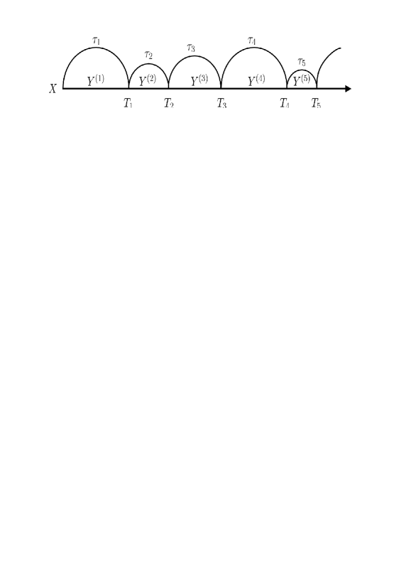
Fix , and satisfying (1.2). Let be i.i.d. -valued random variables with marginal law , and i.i.d. -valued random variables with marginal law . Assume that and are independent, and write to denote their joint law. Cut words out of the letter sequence according to (see Fig. 5), i.e., put
| (2.1) |
and let
| (2.2) |
Under the law , is an i.i.d. sequence of words with marginal distribution on given by
| (2.3) | ||||
The reverse operation of cutting words out of a sequence of letters is glueing words together into a sequence of letters. Formally, this is done by defining a concatenation map from to . This map induces in a natural way a map from to , the sets of probability measures on and (endowed with the topology of weak convergence). The concatenation of equals , as is evident from (2.3).
2.1 Annealed LDP
Let be the set of probability measures on that are invariant under the left-shift acting on . For , let be the periodic extension of the -tuple to an element of . The empirical process of -tuples of words is defined as
| (2.4) |
where the supercript indicates that the words are cut from the latter sequence . For , let be the specific relative entropy of w.r.t. defined by
| (2.5) |
where denotes the projection of onto the first words, denotes relative entropy, and the limit is non-decreasing.
For the applications below we will need the following tilted version of :
| (2.6) |
Note that, for , has a tail that is exponentially bounded. The following result relates the relative entropies with and as reference measures.
Lemma 2.1
[3] For and ,
| (2.7) |
This result shows that, for , whenever , which is a special case of [1], Lemma 7.
The following annealed LDP is standard (see e.g. Dembo and Zeitouni [6], Section 6.5).
Theorem 2.2
For every , the family , , satisfies the LDP on with rate and with rate function given by
| (2.8) |
This rate function is lower semi-continuous, has compact level sets, has a unique zero at , and is affine.
2.2 Quenched LDP
To formulate the quenched analogue of Theorem 2.2, we need some more notation. Let be the set of probability measures on that are invariant under the left-shift acting on . For such that , define
| (2.10) |
Think of as the shift-invariant version of obtained after randomizing the location of the origin. This randomization is necessary because a shift-invariant in general does not give rise to a shift-invariant .
For , let denote the truncation map on words defined by
| (2.11) |
i.e., is the word of length obtained from the word by dropping all the letters with label . This map induces in a natural way a map from to , and from to . Note that if , then is an element of the set
| (2.12) |
Define (w-lim means weak limit)
| (2.13) |
i.e., the set of probability measures in under which the concatenation of words almost surely has the same asymptotic statistics as a typical realization of .
Theorem 2.3
(Birkner [1]; Birkner, Greven and den Hollander [2]) Assume (1.2–1.4). Then, for –a.s. all and all , the family of (regular) conditional probability distributions , , satisfies the LDP on with rate and with deterministic rate function given by
| (2.14) |
and
| (2.15) |
where
| (2.16) |
This rate function is lower semi-continuous, has compact level sets, has a unique zero at , and is affine.
3 Variational formulas for excess free energies
This section uses the LDP of Section 2 to derive variational formulas for the excess free energy of the quenched and the annealed version of the combined model. The quenched version is treated in Section 3.1, the annealed version in Section 3.2. The results in Sections 3.1–3.2 are used in Section 3.3 to prove Theorem 1.1.
In the combined model words are made up of letters from the alphabet , where and are subsets of , and are cut from the letter sequence , where and are i.i.d. sequences of -valued and -valued random variables with joint common law . Let and be the projection maps from onto and , respectively, i.e and for . These maps extend naturally to , , , and . For instance, if , i.e., , then and .
As before, we will write , and for a quantity associated with the copolymer with pinning model, the copolymer model, respectively, the pinning model. For instance, if , and , then the rate functions , , and the sets , , are defined as in (2.13).
The LDPs of the laws of the empirical processes and can be derived from those of via the contraction principle (see e.g. Dembo and Zeutouni [6], Theorem 4.2.1), because the projection maps and are continuous. In particular, for any and
| (3.1) |
where and . Similarly, we may express and in terms of .
3.1 Quenched excess free energy
Abbreviate
| (3.2) |
Theorem 3.1
Assume (1.2) and (1.4). Fix , ,
and .
(i) The quenched excess free energy is given by
| (3.3) |
where
| (3.4) |
with
| (3.5) | |||||
| (3.6) | |||||
| (3.7) |
Here, the map is the projection onto the first
letter of the first word in the sentence consisting of words cut out from , i.e.,
, while the map
is the projection onto the first word in the sentence consisting of words cut out
from , i.e., , and is the length
of the first word.
(ii) An alternative variational formula at is with
| (3.8) |
(iii) The map is lower semi-continuous, convex and non-increasing on , is infinite on , and is finite, continuous and strictly decreasing on .
Proof. The proof is an adaptation of the proof of Theorem 3.1 in [3] and comes in 3 steps.
1. Suppose that has excursions away from the interface. If denote the times at which visits the interface, then the Hamiltonian reads
| (3.9) |
where is the event that the -th excursion is below the interface and . Since each excursion has equal probability to lie below or above the interface, the -th excursion contributes
| (3.10) |
to the partition sum , where is the word in cut out from by the -th excursion interval . Consequently, we have
| (3.11) |
Therefore, summing over , we get
| (3.12) |
with
| (3.13) | ||||
where
| (3.14) |
denotes the empirical process of -tuples of words cut out from by the successive excursions, and are defined in (3.5–3.7).
2. The left-hand side of (3.12) is a power series with radius of convergence (recall (1.8)). Define
| (3.15) |
and note that the limsup exists and is constant (possibly infinity) -a.s. because it is measurable w.r.t. the tail sigma-algebra of (which is trivial). Note from (3.13) and (3.15) that
| (3.16) |
By (1.8), the left-hand side of (3.12) is a power series that converges for and diverges for . Further, it follows from the first equality of (3.13) and (3.16), that the map is non-increasing. In particular, it is strictly decreasing when finite. This we show in Step 3 below. Hence we have
| (3.17) |
3. We claim that, for any and , the map is finite on and infinite on (see Fig. 6), and
| (3.18) |
Note from the contraction principle in (3.1) that and are finite whenever . Therefore, for any , and , it follows from Lemmas A.1 and A.3 in Appendix A that whenever . This implies that the map is convex and lower semi-continuous, since, by (3.4), is the supremum of a family of functions that are finite and linear (and hence continuous) in . Now the fact that is strictly decreasing when finite follows as follows: Suppose that , and . Then it follows from the fact and (3.4) that
| (3.19) |
Further, we will show in Section 6.1 that , for all . This and convexity imply continuity on These prove (iii) of the theorem.
(1)
(2)
(3)
Analogues of Theorem 3.1 also hold for the copolymer model and the pinning model. The copolymer analogue is obtained by putting , which leads to analogous variational formulas for and . In the variational formula for we replace by in (3.4). This replacement is a consequence of the contraction principle in (3.1). Although the contraction principle holds on , it turns out that the play no role in (3.4). Similarly, Theorem 3.1 reduces to the pinning model upon putting . The variational formula for is the same as that in (3.4), with replaced by .
3.2 Annealed excess free energy
We next present the variational formula for the annealed excess free energy. This will serve as an object of comparison in our study of the quenched model. Define
| (3.20) |
(recall (1.4)).
Theorem 3.2
Proof. The proof comes in 3 steps.
Replacing by in (3.12), we obtain from (3.13) that
| (3.23) |
It therefore follows from (3.16) and (3.23) that
| (3.24) |
where
| (3.25) |
Note from (3.20) and (3.25) that the map is non-increasing. Moreover, for any and , we see from (3.12) after replacing by that is the smallest -value at which changes sign, i.e.,
| (3.26) |
The proof of (i) and (ii) will follow once we show that
| (3.27) |
since (3.20), (3.25) and (3.27) show that the map is infinite whenever , and is finite otherwise. Lower semi-continuity and convexity of this map follow from (3.22), because the function under the supremum is linear and finite in , while convexity and finiteness imply continuity. The proof of (3.27) follows from the arguments in [3], Theorem 3.2, as we show in steps 2–3.
2. For the case , note from (3.20) that for all and . To show that for this case, we proceed as in steps (II) and (III) of the proof of [3], Theorem 3.2, by evaluating the functional under the supremum in (3.22) at with
| (3.28) |
where , , , and (recall (1.4))
| (3.29) |
Note from (3.5) that because has zero mean. This leads to a lower bound on that tends to infinity as . To get the desired lower bound, we have to distinguish between the cases and . For use , for with use .
3. For the case , we proceed as in step 1 and 2 of the proof of Theorem 3.2 of [3]. Note that and defined in (3.5–3.7) are functionals of , where is the first-word marginal of . Moreover, by (2.5),
| (3.30) |
with the infimum uniquely attained at , where the right-hand side denotes the relative entropy of w.r.t. . (The uniqueness of the minimum is easily deduced from the strict convexity of relative entropy on finite cylinders.) Consequently, the variational formula in (3.22) becomes
| (3.31) |
where (by an abuse of notation) is the disorder in the first word, is defined in (3.7), , is the length of the word , and
| (3.32) |
Note from (3.20) that . The infimum in the last equality of (3.31) is uniquely attained at . Therefore the variational problem in (3.22) for takes the form
| (3.33) |
The last formula proves (1.15).
As in the quenched model, there are analogous versions of Theorem 3.2 for the annealed copolymer model and the annealed pinning model. These are obtained by putting either or , replacing by and , respectively. The copolymer version of Theorem 3.2 was derived in [3], Theorem 3.2, and the pinning version (for only) in [5], Theorem 1.3.
Putting , we get the copolymer analogue of (3.33):
| (3.34) |
This expression, which was obtained in [3], is plotted in Fig. 7. Putting , we get the pinning analogue:
| (3.35) |
(1)
(2)
(3)
The map has the same qualitative picture as in Fig. 7, with the following changes: the horizontal axis is located at instead of zero, and is replaced by .
Subtracting from (3.34) and (3.35), we get from (3.21) that the excess free energies and take the form given in (1.16) and (1.17), respectively. The following lemma summarizes their relationship.
Lemma 3.3
For every and (recall (1.21))
| (3.36) |
3.3 Proof of Theorem 1.1
Proof.
Throughout the proof , and are fixed.
(i) Use Theorems 3.1(i,iii).
(ii) Recall from (1.11) and (3.3) that
| (3.37) |
Indeed, it follows from (3.3) that is equivalent to saying that the map changes sign at zero. This sign change can happen while is either zero or negative (see Fig. 6(2–3)). The corresponding expression for is obtained in a similar way.
4 Key lemma and proof of Corollary 1.2
The following lemma will be used in the proof of Corollary 1.2.
Lemma 4.1
Fix , and . Then, for ,
| (4.1) |
4.1 Proof of Corollary 1.2
Proof. (ii) Throughout the proof, , and . It follows from (3.36) that .
Note that, for , the map changes sign at some , i.e., for all and (see (3.36)). Hence .
Note from (3.33) and (3.34) that
| (4.2) |
Furthermore, note from Fig. 7(2–3) that, for , the map changes sign at while is either negative or zero. In either case, we need
| (4.3) |
to ensure that the map changes sign at a positive -value. This concludes the proof that .
(i) As we saw in the proof of (ii), for the map to reach zero we need that . Thus, for this range of -values, we know that the map changes sign when it is zero. The proof for follows from Fig. 6.
(iii) We first consider the cases: (a) ; (b) and . In these cases we have that by (ii). It follows from (3.33–3.34) and Fig. 7 that the map changes sign at some while it is either zero or negative. In either case the finiteness of the map on and (4.1) imply that changes sign at a smaller value of than does. This concludes the proof for cases (a–b).
We next consider the case: (c) with , and . We know from (4.1) that for and . If , then the map changes sign at while jumping from to . By the continuity of the map on , this implies that the map changes sign at a -value smaller than . Furthermore, if , then the map changes sign at a -value larger than , while it is zero. Since for , we have that .
(iv) The proof follows from Lemma 3.3.
4.2 Proof of Lemma 4.1
Proof. The proof comes in five steps. Step 1 proves the strict inequality in (4.1), using a claim about the finiteness of at some specific in combination with arguments from Birker [1]. Steps 2-5 are used to prove the claim about the finiteness of . Note that for the claim trivially follows from Theorems 3.1(iii) and 3.2(ii), since and for this range of -values. Thus, what remains to be considered is the case .
1. For , note from (3.32) and the remark below it that there is a unique maximizer for the variational formula for in (3.22), where
| (4.4) |
where
| (4.5) |
Note further that . We claim that, for and under the conditions in (4.1),
| (4.6) |
This will be proved in Step 2. Let be such that . Then the set
| (4.7) |
is compact in the weak topology, and contains in its interior. It follows from Birkner [1], Remark 8, that is a closed subset of . This in turn implies that there exists a such that (the -ball around ) satisfies . Let
| (4.8) |
Then . Therefore, for and under the conditions in (4.1), we get that
| (4.9) |
The strict inequality follows because no maximizing sequence in can have as its limit ( being the unique maximizer of the variational problem in the second inequality).
2. Let us now turn to the proof of the claim in (4.6). For , it follows from (4.4) and (4.5) that
| (4.10) |
where
| (4.11) |
The inequality in (4.10) follows from (4.4) after replacing by 1. It is easy to see that , because for we have that . Furthermore, since has a finite moment generating function, it follows from the Hölder inequality that . We proceed to show that .
3. We first estimate . Note that
| (4.12) |
where
| (4.13) |
The finiteness of will follow once we show that
| (4.14) |
4. We start with the estimation of . Put and, for and , define
| (4.15) |
Then note that
| (4.16) |
The second inequality uses that on and . Estimate
| (4.17) |
The last inequality uses [3], Lemma D.1, where is a positive constant depending on only. Inserting (4.17) into (4.16), we get
| (4.18) |
Furthermore, using that , we get
| (4.19) |
5. We proceed with the estimation of :
| (4.20) |
where . The right-hand side is non-negative because , and so
| (4.21) |
This bound is finite if
-
1.
;
-
2.
and .
This concludes the proof since, if , then and we only want the finiteness for .
For the pinning model, the associated unique maximizer for the variational formula for satisfies for . However, this does not imply separation between and , since we may have for . The separation occurs at as soon as , since this will imply that .
5 Proof of Corollary 1.3
To prove Corollary 1.3 we need some further preparation, formulated as Lemmas 5.1–5.3 below. These lemmas, together with the proof of Corollary 1.3, are given in Section 5.1. Section 5.2 contains the proof of the first two lemmas, and Appendix C the proof of the third lemma.
5.1 Key lemmas and proof of Corollary 1.3
Lemma 5.1
For ,
| (5.1) |
Furthermore, the map is strictly convex and strictly decreasing on .
Lemma 5.2
For every and (see Fig. 8),
| (5.2) |
(a)
(b)
Lemma 5.3
For every and (see Fig. 9),
| (5.3) |
We now give the proof of Corollary 1.3.
Proof. Throughout the proof , and are fixed. Note from (3.7) that the map is strictly decreasing and convex for all . It therefore follows from (3.4) and (3.22) that the maps and are strictly decreasing when finite (because ) and convex (because sums and suprema of convex functions are convex).
Recall from (1.14) and (3.3) that
| (5.4) |
Indeed, it follows from (3.3) that is equivalent to saying that the map changes sign at zero. This change of sign can happen while is either zero or negative (see e.g. Fig. 6(2–3)).
For , it follows from Lemma 5.1 and Fig. 8 that is the smallest value of at which and hence . Furthermore, note from Fig. 8 that the map is strictly decreasing and convex on and has the interval as its range. In particular, and . Therefore, for , the map changes sign at the unique value of at which .
The proof for follows from that of after replacing , and by , and , respectively.
Since both the quenched and the annealed free energies are convex functions of (by Hölder inequality), and are also convex and strictly decreasing.
5.2 Proof of Lemmas 5.1–5.2
Proof of Lemma 5.2:
Proof.
Throughout the proof and are fixed. The proof uses arguments
from [3], Theorem 3.3 and Section 6. Note from (3.16),
(3.18) and Lemma B.1 that
| (5.7) |
where
| (5.8) |
It follows from the fractional-moment argument in [3], Eq. (6.4), that
| (5.9) |
where is chosen such that . Abbreviate the term inside the brackets of (5.9) by and note that
| (5.10) |
Therefore, for , this estimate together with the Borel-Cantelli lemma shows that -a.s. (recall (2.6))
| (5.11) |
This estimate also holds for when . This is the case for any pair and satisfying (recall (1.2)). Therefore we conclude that whenever .
To prove that for , we replace in [3], Eq. (6.8), by
| (5.12) |
where
| (5.13) |
With this choice the rest of the argument in [3], Section 6.2, goes through easily.
Finally, to prove that at we proceed as follows. Adding, respectively, and to the functionals being optimized in [3], Eqs. (6.19–6.20), we get the following analogue of [3], Eq. (6.21),
| (5.14) |
where
| (5.15) |
Note from [3], Eqs. (6.23–6.29), that . Therefore it follows from [3], Steps 1 and 2 in Section 6.3, that
| (5.16) |
6 Proofs of Corollaries 1.4–1.8
6.1 Proof of Corollary 1.4
Proof. Throughout the proof, , , and are fixed. The proof for is trivial, since and . The rest of the proof will follow once we show that for . This is because, for , and is non-increasing. Furthermore, the map is also non-increasing, and so .
For , it follows from Corollary 1.3 that is the unique -value that solves the equation . Note that for , which is the range of -values attainable by , the measure (recall (3.32)) is well-defined and is the unique minimizer of the last variational formula in (3.31), for . Hence, for , is the unique -value that solves the equation
| (6.1) |
Again, it follows from (2.18) that, for any ,
| (6.2) |
Furthermore, it follows from (2.5) and the remark below it that
| (6.3) |
where is the projection onto the first letter and . Moreover, it follows from (2.10) that
| (6.4) |
Since , (6.3–6.4) combine with (3.8) to give
| (6.5) |
where
| (6.6) |
and
| (6.7) |
with the notation
| (6.8) |
and
| (6.9) |
Therefore, for , after combining the first two terms in the supremum in (6.5), as in (3.31), we obtain
| (6.10) |
Hence, for , it follows from (3.31) that
| (6.11) |
The first term in the variational formula achieves its minimal value zero at (or along a minimizing sequence converging to ). However, via some simple computations we obtain
| (6.12) |
where
| (6.13) |
and . Here we use that
| (6.14) |
with
| (6.15) |
Note that , where . Thus for , and so we have
| (6.16) |
Since and since is strictly decreasing on , it follows that for .
6.2 Proof of Corollary 1.5
6.3 Proof of Corollary 1.6
6.4 Proofs of Corollaries 1.7 and 1.8
Proof. The proofs are similar to those of Corollaries 1.6–1.7 in [3], Section 8. For the former, all that is needed is , which holds for .
Appendix A Finiteness of
Lemma A.1
Fix and satisfying (1.4). Then, for all with , there are constants and such that
| (A.1) |
Proof. The proof comes in 3 steps.
1. Abbreviate
| (A.2) |
Fix . For and , define
| (A.3) | ||||
Note that the ’s and the ’s are pairwise disjoint, and that
| (A.4) |
where and denote the set of positive and negative real numbers in . Also note that
| (A.5) | ||||
where
| (A.6) | ||||
The term follows from the restriction of the -integral to the set . The terms and follow from the restrictions to the sets and . The bound on uses that on and on . The bound on follows from the fact that on and on . It follows from (A.6) that
| (A.7) | ||||
where the third inequality uses (1.4). Moreover, use that on , to estimate
| (A.8) |
where the third inequality uses that on , and the second equality that
| (A.9) |
Put
| (A.10) |
2. Similarly, we have
| (A.11) | ||||
where
| (A.12) | ||||
The bounds on and use that on and on . Note that
| (A.13) | ||||
Also use that on , to estimate
| (A.14) |
3. Put . Then the claim follows with .
For the sake of completeness we state the follow finiteness results for that were proved in [3], Appendix A.
Lemma A.2
Fix . Then -a.s. there exists a such that, for all and for all sequences ,
| (A.15) |
where is the word cut out from by the th excursion interval .
Appendix B Application of Varadhan’s lemma
In this appendix we prove (3.18) and the claim above it. This was used in Section 3 to complete the proof of Theorem 3.1.
Lemma B.1
Proof. Throughout the proof , and are fixed. The proof comes in 3 steps, where we establish the equality in (B.1) for the cases , and separately.
Step 1. For the proof of (B.1) is given in two steps.
1a. In this step we show that when . Fix and let , with
| (B.2) |
and It follows from (3.4) that
| (B.3) |
The second inequality uses that , and . Letting and using that has a polynomial tail by (1.2), we get the claim.
1b. In this step we show that when . The proof follows from a moment estimate. We start by showing that, for each ,
| (B.4) |
(recall (1.4)). Indeed, for any , by the Markov inequality,
| (B.5) |
The claim therefore follows from the Borel-Cantelli lemma. Note from (B.5) that (B.4) holds if we replace with ,
Let be the length of the -th word, let , and put
| (B.6) |
For any with and , it follows from (3.13) that
| (B.7) | ||||
where
| (B.8) |
The first inequality in (B.7) uses that , and . The second inequality follows from the reverse Hölder inequality with the above choice of and . Note that is finite for and . It therefore follows from (3.16), (B.4) and (B.7) that
| (B.9) |
Letting , we get from (2.6) that , since for .
Step 2. In this step, which is divided into 2 substeps, we consider the case .
2a. Lower bound: For , define
| (B.10) |
Note that is lower semi-continuous and that
| (B.11) |
Therefore, for any with , it follows from the Hölder inequality that
| (B.12) |
The rest of the proof consists of taking the appropriate limits and showing that the left-hand side of (B.12) is bounded from below by , while the second term in the right-hand side tends to zero and the first term tends to .
Let us start with the second term in the right-hand side of (B.12). Note from (2.6) that
| (B.13) |
The first inequality uses the Cauchy-Schwarz inequality, the second inequality uses (B.4). Note from (1.4) that the above bound tends to zero upon when followed by .
For the first term in the right-hand side of (B.12) we proceed as follows. Note from Lemma A.2 that -a.s.
| (B.14) |
where we use that
| (B.15) |
Therefore, for any , it follows from (B.4) and (B.14) that -a.s.
| (B.16) |
Next, for with , it follows from the argument leading to (B.9) that
| (B.17) |
since . Define
| (B.18) |
By (B.16–B.17), the map is convex and finite on , and hence continuous on . It therefore follows from (3.15) that the left-hand side of (B.16) converges to as . It follows from (B.16–B.17) that this limit is finite, which proves the finiteness of the map on .
Finally, we turn to the left-hand side of the inequality in (B.12). For any and , note from the lower semi-continuity of the map that the set
| (B.19) |
is open. This implies that
| (B.20) |
The second inequality uses Theorem 2.3, the third inequality uses that , the fourth inequality follows from the fact that , while the equality follows from Lemma 2.9. It therefore follows from (B.12–B.13), (B.20) and the comment below (B.18) that, after taking the supremum over followed by , and ,
| (B.21) |
2b. Upper bound: Let . For , define
| (B.22) |
Note that and are upper semi-continuous and
| (B.23) |
Therefore, for any with , the reverse Hölder inequality gives
| (B.24) |
The rest of the proof for the upper bound follows after showing that the left-hand side of (B.24) gives rise to the desired upper bound, while the right-hand side gives rise to after taking appropriate limits.
It follows from [3], Step 2 in the proof of Lemma B.1, that
| (B.25) |
for large enough. Hence, for large enough, it follows from (B.4), (B.25) and that
| (B.26) |
which tends to zero as followed by . Furthermore, it follows from (B.16–B.18) and the remark below (B.18) that
| (B.27) |
Since is upper semi-continuous, it follows from Dembo and Zeitouni [6], Lemma 4.3.6, and Theorem 2.3 that
| (B.28) |
The first equality uses that for (recall (2.14)) and the fact that , the second equality uses (2.9) and the fact that on . (The removal of ’s with again follows from ), the last inequality uses that and . Therefore, combining (B.24–B.28) and letting and in the appropriate order, we conclude the proof of the upper bound.
Step 3. For we show that
| (B.29) |
(recall (3.8)). The first equality follows from Steps 1 and 2 of the proof. The second uses that the map is decreasing and lower semi-continuous on .
Furthermore, note from (3.4) and (3.8) that
| (B.30) |
Here we use that on . The rest of the proof will follow once we show the reverse of (B.30). To do so we proceed as follows:
For and , with , it follows from (3.15) and the reverse Hölder inequality that
| (B.31) |
Here, is defined in (B.10). The second inequality uses Steps 1 and 2 of the proof, particularly (B.4) and the remark below (B.5).
Below we show that, for any and ,
| (B.32) |
Therefore, upon taking limits in the order , and , it follows from (B.31, B.32) and the lower sime-continuity of the map on that
| (B.33) |
Lemma B.2
Suppose that is finite. Then for every there exists a sequence in such that and , where and means weak limit.
In our case .
For the rest of the proof we proceed as in [3], Appendix C. For , let
| (B.34) |
be a grid of spacing in , which represents a finite set of letters approximating . Put and let be the set of finite words drawn from . Furthermore, let and be the letter maps
| (B.35) | ||||
Thus, moves points upwards on , while does the opposite on . Let be such that , for all . This map naturally extends to , and to the sets of probability measures on them. Furthermore, put , ,
| (B.36) | ||||
where
| (B.37) | ||||
Here, is the projection onto the first word in the word sequence formed by the copolymer disorder , and is the projection onto the first letter of the first word in the word sequence formed by the pinning disorder .
Next, note from (B.31) that
| (B.38) |
For the rest of the proof we assume that . Consider a combined model with disorder taking values in instead of , and with and replaced by and , respectively. In this set-up, if in (B.38) we replace and by and respectively, then we obtain
| (B.39) |
Here, is the empirical process of -tuple of words cut out from the i.i.d. sequence of letters drawn from according to the marginal law . Note from (B.10) that
| (B.40) | ||||
It therefore follows from (B.38–B.39) that
| (B.41) |
In the sequel we will write, respectively, , , , associated with and as the analogues of , , , associated with and . It follows from Steps 1 and 2 above that
| (B.42) |
Note from Lemma B.2 that for any with there exists a sequence in such that and , because is finite. Therefore
| (B.43) | ||||
The first equality uses the second equality of (B.29) and the remark below it. The
third equality uses the above remark about Lemma B.2, the boundedness and the
continuity of the map
on , and the fact that
on . Note also that those ’s
with do not contribute to the above supremum. For each
, define Since is a projection map we have that
. It therefore follows from (B.43) that
| (B.44) | ||||
Appendix C Proof of Lemma 5.3
In this Appendix we prove Lemma 5.3. To do so we need another lemma, which we state and prove in Section C.1. In Section C.2 we use this lemma to prove Lemma 5.3.
C.1 A preparatory lemma
Lemma C.1
For every , and ,
| (C.1) |
where
| (C.2) |
and is the word length distribution under .
Proof. Throughout the proof, , and are fixed. Put
| (C.3) |
Note from (B.5) and the Borel-Cantelli lemma that, for every and -a.s., there exists an such that
| (C.4) |
Therefore, -a.s. and for all ,
| (C.5) |
Finiteness follows from (C.4) and the fact that if . Therefore, for every , -a.s. and , we have
| (C.6) |
From the Borel-Cantelli lemma we therefore obtain that -a.s.
| (C.7) |
The equality uses Steps 1 and 2 in the proof of Lemma B.1 and the observation that is independent of (i.e., only pinning disorder is present), and for , where we use (2.15) instead of (2.14). Finally, let .
C.2 Proof of Lemma 5.3
Proof. Throughout the proof, and are fixed and . Note from (3.6) and (3.7) that . Therefore, replacing by in (3.8), we get
| (C.8) |
The fourth equality follows from the proof of Lemma B.1, while the last equality uses [5], Theorem 1.3. Next, note that
| (C.9) |
since the map is non-increasing. For it follows from (C.1) that
| (C.10) |
The third inequality uses that, for , for all . Therefore
| (C.11) |
References
- [1] M. Birkner, Conditional large deviations for a sequence of words, Stoch. Proc. Appl. 118 (2008) 703–729.
- [2] M. Birkner, A. Greven and F. den Hollander, Quenched LDP for words in a letter sequence, Probab. Theory Relat. Fields 148 (2010) 403–456.
- [3] E. Bolthausen, F. den Hollander and A.A. Opoku, A copolymer near a selective interface: variational characterization of the free energy, arXiv:1110.1315.
- [4] F. Caravenna, G. Giacomin and F.L. Toninelli, Copolymers at selective interfaces: settled issues and open problems, in: Probability in Complex Physical Systems, Proceedings in Mathematics, Vol. 11, Springer, Berlin, 2012, pp. 289–310.
- [5] D. Cheliotis and F. den Hollander, Variational characterization of the critical curve for pinning of random polymers, EURANDOM Report 2010–024, arXiv:1005.3661v1, to appear in Ann. Probab.
- [6] A. Dembo and O. Zeitouni, Large Deviations Techniques and Applications (2nd. ed.), Springer, New York, 1998.
- [7] G. Giacomin, Localization phenomena in random polymer models, Preprint 2004. Available online: http://www.proba.jussieu.fr/pageperso/giacomin/pub/publicat.html
- [8] G. Giacomin and F.L. Toninelli, The localized phase of disordered copolymer with adsorption, Alea 1 (2006) 149–180.
- [9] G. Giacomin and F.L. Toninelli, Smoothing of depinning transitions for directed polymers with quenched disorder, Phys. Rev. Lett. 96 (2006) 070602.
- [10] G. Giacomin and F.L. Toninelli, Smoothing effect of quenched disorder on polymer depinning transitions, Commun. Math. Phys. 266 (2006) 1–16.
- [11] G. Giacomin, Random Polymer Models, Imperial College Press, World Scientific, London, 2007.
- [12] F. den Hollander, Random Polymers, Lecture Notes in Mathematics 1974, Springer, Berlin, 2009.
- [13] N. Pétrélis, Copolymer at selective interfaces and pinning potentials: weak coupling limits, Ann. Inst. H. Poincaré 45 (2009) 175–200.
- [14] F.L. Toninelli, Disordered pinning models and copolymers: beyond annealed bounds, Ann. Appl. Probab. 18 (2008) 1569–1587.