Swarming and Pattern Formation due to Selective Attraction and Repulsion
Abstract
We discuss the collective dynamics of self-propelled particles with selective attraction and repulsion interactions. Each particle, or individual, may respond differently to its neighbors depending on the sign of their relative velocity. Thus, it is able to distinguish approaching (coming closer) and moving away individuals. This differentiation of the social response is motivated by the response to looming visual stimuli and may be seen as a generalization of the previously proposed, biologically motivated, escape and pursuit interactions. The model can account for different types of behavior such as pure attraction, pure repulsion, or escape and pursuit depending on the values (signs) of the different response strengths, and provides, in the light of recent experimental results, an interesting alternative to previously proposed models of collective motion with an explicit velocity-alignment interaction. We show the onset of large scale collective motion in a subregion of the parameter space, which corresponds to an effective escape and/or pursuit response. Furthermore, we discuss the observed spatial patterns and show how kinetic description of the dynamics can be derived from the individual based model.
pacs:
05.40.-a,87.16.Uv,87.18.TtI Introduction
Collective motion in biology, as observed for example in flocks of birds, schools of fish or within bacterial colonies, is a fascinating display of natural self-organization. Over the years, it has been the topic of numerous scientific publications addressing it from very different angles and with different questions in mind, both experimentally and theoretically. From a more biological perspective the interesting questions are the evolutionary advantages and the biological and ecological function of collective behavior in various species Couzin et al. (2002); Krause and Ruxton (2002); Yates et al. (2009); Bazazi et al. (2011), whereas physicist addresses rather the question about universal laws and phase-transition behavior in minimal models of collective motion Vicsek et al. (1995); Toner and Tu (1995, 1998); Grégoire and Chaté (2004); Aldana et al. (2007); Chaté et al. (2008); Romanczuk et al. (2009, 2012). The design, control and stability of collective dynamics in multi-agent systems is also a major research topic in engineering Leonard et al. (2007); Sepulchre et al. (2008); Turgut et al. (2008); Ferrante et al. (2011), and the general properties of related mathematical models are under active investigation in mathematics Cucker and Smale (2007); Carrillo et al. (2010).
Most of the mathematical models for collective motion proposed in the literature, contain some sort of explicit velocity-alignment mechanisms, which tends to align the velocity of a focal individual with the velocity of its neighbors Niwa (1994); Vicsek et al. (1995); Couzin et al. (2002, 2005); Romanczuk et al. (2008); Bode et al. (2010). However, recent experimental studies of collective behavior in fish do not find any clear evidence for the existence of an explicit velocity-alignment interaction Herbert-Read et al. (2011); Katz et al. (2011). Only relatively few models, have analyzed the onset of collective motion without an explicit alignment mechanisms based on purely repulsive and attractive interactions (see e.g. Ebeling and Schweitzer (2001); Peruani et al. (2006); Grossman et al. (2008); Strefler et al. (2008); Strömbom (2011)). Recently, motivated by empirical evidence for cannibalism as the driving force of collective migration in certain insect species Simpson et al. (2006); Bazazi et al. (2008), we have proposed a model of collective motion based on escape and pursuit responses Romanczuk et al. (2009); Bazazi et al. (2011). In this escape-pursuit model, individuals are reacting to their neighbors by moving away from others approaching them from behind (escape), and/or increasing their velocity towards those who are moving away in front of them (pursuit). This kind of social response requires individuals to distinguish between approach and movement away as well as between individuals in front and behind them. This previous model can be considered to belong to a broader class of selective attraction-repulsion models, which we believe are very promising for theoretical modelling of collective motion in biology. Here we discuss and analyze a generalization of the original escape-pursuit model to the case where self-propelled agents (or particles) are responding selectively to approaching and moving individuals without taking their relative position into account Guttal et al. (2012). Furthermore, we do not put any restrictions on the sign (direction) of the effective social forces modelling the selective response. This allows to account for different social behavior types, such as pure attraction, pure repulsion and escape and pursuit, in a single model, by the same set of social forces, only by changing the values of the response strengths.
We will start with the definition of the individual based model in terms of stochastic differential equations and continue with the derivation of a kinetic description of the system. Finally, we will discuss simulation results with a particular focus on the emergence of large-scale collective motion.
II Individual Based Model
We consider a system of self-propelled particles in two spatial dimensions, which move with a constant speed in a spatial domain of size with periodic boundary conditions. The interaction between different particles (individuals) is modelled as an effective social force . The evolution of the system is determined by the following equations of motion for the positions and the polar orientation angle , which determines the direction of the heading unit vector :
| (3) | ||||
| (4) |
The temporal evolution of is determined by the turning of the individual due to social interactions and random (angular) fluctuations with the intensity . The (angular) social force is given by the projection of the total social force vector on the angular degree of freedom with . The angular noise is Gaussian white noise with zero mean and vanishing temporal correlations.
The total social force is given by a sum of three components:
| (5) |
The first term represents a short range repulsion responsible for collision avoidance. It reads
| (6) |
with being a constant repulsive turning rate. The Heaviside function ensures that the repulsion takes place only if the distance between the focal individual and the respective neighbor is below the repulsion distance . The total repulsive response is normalized by the number of individuals within the repulsion distance
| (7) |
The other two forces read:
| (8) | ||||
| (9) |
Both forces represent averaged two-individual interactions, which act always along the unit vector pointing towards the center of mass of the neighboring particle . The first one, , represents the response to approaching individuals characterized by a negative relative velocity . The second, , is the corresponding response to moving away (or receding) individuals characterized by positive relative velocity . This differentiation is reflected by the last Heaviside functions . The two other step functions are identical for both interactions and restrict these social responses to neighbors within a sensory range but outside the repulsion zone. The parameters determine the turning rates due to the respective interaction. Both force terms are proportional to the relative velocity, which lead to stronger responses to faster approaching or receding individuals. Furthermore, they are normalized by the respective number of individuals for the corresponding interaction type:
| (10) |
Here, we used for simplicity step-like functions for the spatial dependence of the different interaction. The general results will not be altered by other smooth functions of the distance as long as they decay sufficiently fast in order to ensure local interactions. Please note that the definition of the step-like interaction zones resembles the two-zone model introduced by Couzin and co-workers Couzin et al. (2005, 2011). However, the model discussed here does not contain an explicit velocity-alignment.
A schematic visualization of the interaction scheme with the differentiation between approach and moving away is given in Fig 1.
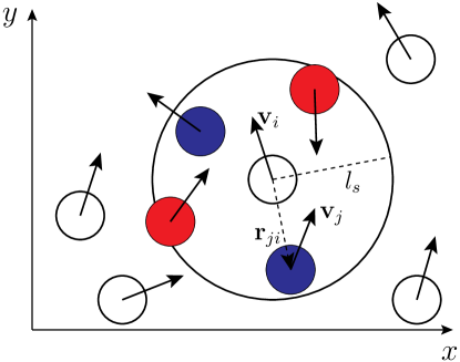
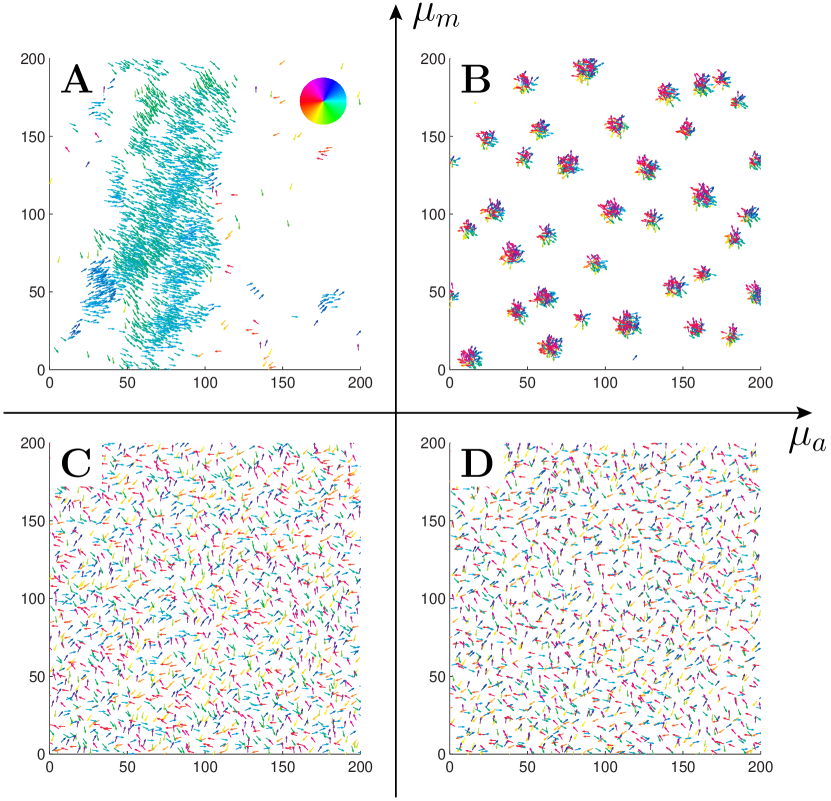
The social forces can lead independently to a repulsive (attractive) response to approaching individuals for () and a repulsion (attraction) to individuals moving away (). In the -parameter space we distinguish the four quadrants corresponding to different behavior types (see also Fig. 2):
-
i.
Pure Repulsion: repulsion from approaching and moving away individuals: and .
-
ii.
Escape and Pursuit: repulsion from approaching individuals , attraction to moving away individuals .
-
iii.
“Head on Head”: attraction to approaching individuals , repulsion from moving away individuals .
-
iv.
Pure Attraction: attraction to approaching and moving away individuals: and .
There exist also the special cases with and (), which correspond to a selective attraction (repulsion) only to approaching/moving away individuals, and the case of particles interacting only via short-range repulsion ().
We refer to the situation and as “Escape and Pursuit”, due similar behavior as in the original Brownian particle model Romanczuk et al. (2009). For and the social forces lead to a preference to move towards other individuals which already are coming closer and therefore favor (in particular at low densities) frontal collisions between individuals. We refer to this regime as “Head on Head”.
III Kinetic Description
In this section we derive a kinetic description for the above individual based model. For this purpose we introduce the -particle probability density function (PDF)
which determines the probability to find a particle (individual) at time , at position , with velocity pointing in direction (). It is normalized with respect to integration over space and over all angles. Further on, for simplicity, we assume that correlations between particles can be neglected. Therefore, the -particle distribution density shall factorize, i.e. . In agreement with (3) and (4), we can write down the Fokker-Planck equation (FPE) for the PDF of the -th particle
| (11) |
with being the unit vector in the heading direction of individual , and being the angular unit vector perpendicular to . The above FPE is nonlinear since the interaction force depends on the probability density for the position and the velocity angle of the particles within their sensory range.
We will now reduce the description to moments of the one-particle PDF, which are the particle density
| (12) |
and the expectation values of the cosine and sine of the velocity angle defined as
| (13) |
where the conditional probability density function of the velocity direction is defined through the relation . Similar approach was previously used in the context of swarming of Active Brownian Particles in Romanczuk and Erdmann (2010); Romanczuk and Schimansky-Geier (2011); Grossmann et al. (2012).
Integrating the Fokker-Planck equation (11) over the velocity-angle yields the continuity equation which reads
| (14) |
Similarly, we derive the equations for the angular moments
| (15) | |||||
| (16) | |||||
Here, we introduced the averaging over the conditional PDF as which are functions of the position and time. The second moments of the trigonometric functions of the direction angle read
| (17) |
The approximation for the second moments indicated on the r.h.s. of the above equation, will be used later on. It neglects higher harmonics in the equation of motion for the angular PDF, which essentially restricts the analysis to the relaxation of the slowest (fundamental) modes of the angular PDF.
In order to obtain an equation for the density, we insert the equations of the angular moments into the continuity equation. For this purpose, we take the temporal derivative of the spatial density for a second time
| (18) | |||
If we introduce in this equations abbreviations for the variances of the second angular moments defined as
| (19) |
the equation for the density becomes
| (20) |
We note, one still needs equations or expressions for the variances which have to be inserted.
Similarly, we separate the density from the angular moments using the continuity equation. After a few steps, one obtains the equation of motion for the mean cosine
| (21) |
and for the mean sine
| (22) |
respectively. We multiply the first equation (III) by the mean cosine and the second one (III) by the mean sine and obtain the equation for the order parameter:
| (23) | |||
The only term, which can induce an instability of the homogeneous, disordered solution in Eqs. (18) and (III) contains the interaction force. The remaining terms, which contain only the zeroth up to second moments of the orientation, are present also in the case of non-interacting particles. They describe the relaxation dynamics of the resulting patterns towards a steady state, but are not the source of an eventual inhomogeneous solutions.
We see that a further analysis needs still the treatment of integrals which contain the interaction forces, which can be very tedious in the general case. Further below, we will consider principal cases where and have the same absolute value and differ only in their sign and derive approximations for the respective integrals.
The force changing the direction of the th-particle can be formulated by introducing an interaction parameter depending of the distance between particles and their relative velocities. We define
| (24) |
where is the distance between from the th to the th particle and again the relative velocity projected on the distance vector. Otherwise, this function vanishes. The have to be specified for positive and negative relative velocities. They read, in agreement with (8) and (9),
| (25) |
The normalizing numbers in denominators can be expressed as integrals over the respective distances and relative velocities. In detail, with the definition of the total number density as , where is the total volume (area in 2d) one gets
| (26) |
where the are the (effective) partial volumes for the different interaction types, respectively. For the integration one can transform to polar coordinates, integrating over the distance and the polar angle , determining the position of particle with respect to the focal particle .
The force in the third term on the r.h.s. of the Fokker-Planck equation (FPE, Eq. 11) can be expressed as an integral over the probability density of the independent other particles. With the new definition of the interaction parameter, this forces reads
| (27) |
Expressed by the probability density of the interacting particles it becomes
| (28) |
Finally, we derive an expression of the projection of the relative velocity. After a few calculations, one obtains the relative velocity as a function of the velocity angles , and the position angle :
| (29) |
which allows a closure of the kinetic description.
By virtue of the assumptions made, the effective force separates in three parts: one coming from the repulsion at short distances, one from “moving away” and the third, from “approaching” individuals. In the following discussion, we will first restrict ourselves to the second and the third interaction type, which corresponds to a limit of a vanishing short-range repulsion length . In general, the short-ranged repulsion increases the pressure and the effective temperature in the system but does not induce instabilities and inhomogeneous steady states as observed in the simulations (see Sect IV). However, it determines the size of the observed structures.
In the following, we investigate the force turning the velocity angle and project on the unit vector . The integral (28) transforms into
| (30) |
where the spatial distance between the -th and the -th particle appears explicitly in the argument of the PDF. The product between the two unit vectors in (III) can be expressed in terms of the different angles as . Further on, we will also not distinguish from the particle number approaching and moving away by setting .
From Eq. (29) we find the two different regions of integration where the relative velocity has a different sign for in the interval :
| (31) |
Hence, a particle, located in the half-sphere in clockwise direction from the mean angle approaches the focal particle, whereas, a particle located in the other half-sphere counterclockwise from the mean angle are moving away. Thus, the support of the interaction integrals for “approach” and “moving away” corresponds to these two different half-spheres (see Fig 3). Please note that for the social force vanishes as (29).
As an approximation, we will replace this integration by averaged values fixing the probability distribution in the centers of the half-spheres, i.e. at a distance from and with the angle for the approaching particles and correspondingly for particles moving away. The corresponding distance vectors are parallel but point in a different direction. They read
| (32) |
These vectors correspond to the center of mass of approaching (moving away) individuals under the assumption of a homogeneous spatial distribution of neighbors with direction .
We separate the spatial PDF from the distribution of the velocity-angles using the conditional angle PDF, i.e. . Assuming that the density depends only weakly on the position within the sensing region, one can take it constant within the range of spatial integration. Consequently, the spatial integration cancels together with the denominator and we get for the projected force
The resulting expression will be taken in a dipole approximation. Subsequently, we develop the difference in small up to the first derivative which yields two contributions . In first order, we get
| (34) | ||||
The second approximation includes the derivatives in direction of the centers of the half-spheres. Inserting the corresponding directional cosines we obtain in second approximation
| (35) |
and the unit vector of (32) still depends of the velocity angles which have to be taken into account if averaging .
Both orders depend qualitatively different of the social force strengths. Whereas the first order, corresponding to a monopole contribution, depends on the difference of the interaction strengths, the second (dipole contribution) contains the sum of both coefficients. Assuming that both coefficients differ only in their sign, the first order describes effectively a perfectly symmetric “escape and pursuit” (or “Head on Head”) situation. In this case , which depends on the local gradients, vanishes. Thus in this special cases, the effective turning rate does not depend, up to second order, on spatial (density) inhomogeneities. On the other hand for social interactions with equal sign, such as “pure attraction” and “pure repulsion”, the vanishes and only the second order contributes. In this case, there is no monopole force driving the local collective dynamics. However, depending on the sign, the social force can lead to an amplification of density inhomogeneities (“pure attraction”), or will stabilize the spatially homogeneous state (“pure repulsion”). We should mention that the short ranged repulsion is described by a similar expression as for the case of pure repulsion but without the factor .
In the general case of arbitrary and , the resulting dynamics will be a combination of both contributions. However, from the analysis of the dependence of the effective turning as a function of the interaction strengths, it can be easily seen that that the main diagonals and separate qualitatively different regions. For example, in the escape and pursuit quadrant, the second order contribution changes its sign at the diagonal with , which indicates that the social interactions tend to amplify density inhomogeneities in the pursuit dominated region , whereas the opposite is the case in the escape dominated region .
Further on, we will focus for simplicity on the monopole term. The averaged force terms in Eqs. (15) become
| (36) |
and
| (37) |
respectively. With these expressions, the term in the evolution equation of the order parameter (Eq. III) containing the forces becomes proportional to and we obtain
| (38) | |||
One sees that this term is determined by the temperature of the particle gas. The r.h.s. of the given expression can become positive for positive . It describes the creation of order if its value is larger then the effective relaxation process which arises from the noise in the velocity angles.
For an estimation of the critical values of the onset of order one might take the approximation in Eq. (III) which yields that the r.h.s. approaches . Hence, a necessary condition for a growing order parameter, thus onset of collective motion, we obtain
| (39) |
In general, for vanishing fluctuations, collective motion can emerge only above the main diagonal with . With increasing noise strength the regime of collective motion, is predicted to recede into the escape-pursuit regime.
The above result, as well as the formulation of a kinetic description in general, not only provide qualitative insights into the impact of the interaction strengths on the large scale system dynamics, but provide also a starting point for a more quantitative analysis of the stability of the inhomogeneous solutions. However, this requires further assumptions on the properties of the involved probability densities which ensure a closure of the descriptions, e.g. assumptions for the temperature, which are beyond the scope of this work.
IV Simulation Results
In order to characterize the behavior of the model, we have performed systematic numerical simulations for varying interactions strengths (), different densities and noise strengths .
In the following we will discuss our results in term of the dimensionless density , rescaled by the sensory range, which is proportional to the average number of individuals per interaction zone for a homogeneous (random) spatial distribution.
We focus in particular on the question what combinations of , lead to large scale collective motion. The degree of collective motion after the system reaches a steady state is measured using the time averaged center-of-mass speed normalized by the preferred speed of individuals , which is the well-known order parameter used in the analysis of Vicsek-type models:
| (40) |
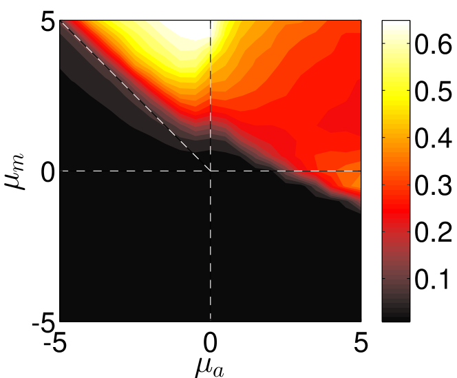
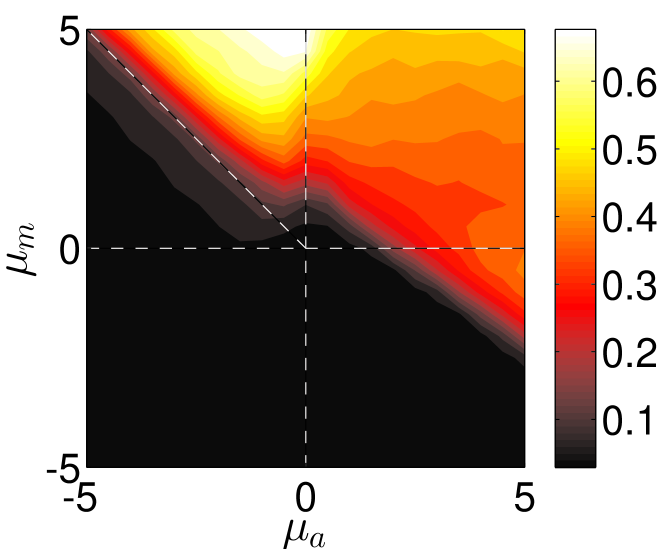
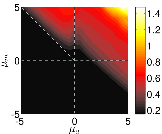
where denotes the temporal average and the ensemble average. In addition, we measure the spatial inhomogeneity (clustering) by the time averaged scaled neighbor number
| (41) |
with being the average number of neighbors within the metric distance given by the sensory range of an individual at a given time . The density-dependent scaling number defines the maximal expectation values for the measured neighbor numbers corresponding to the closest packing of individuals by assuming an impenetrable repulsion zone with a diameter :
| (42) |
Here is the packing fraction for the closest packing of discs in two spatial dimensions. The term in the definition of takes into account that the focal particle is not being counted as its own neighbor. Please note, that as we are considering a soft core interaction, can in principle be larger than one, in particular for high densities and strong attraction.
,
center of mass speed 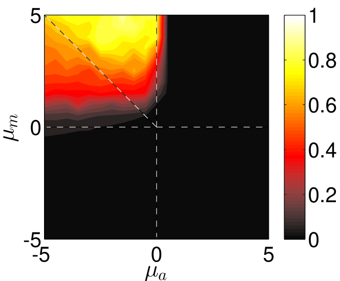 neighbor number
  ,
,
center of mass speed 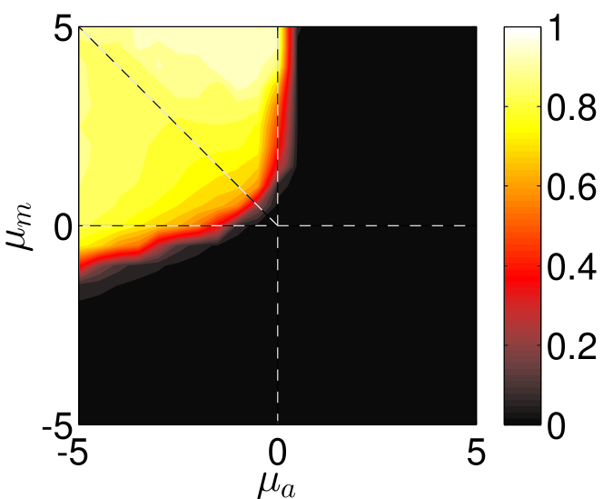 neighbor number
  ,
,
center of mass speed 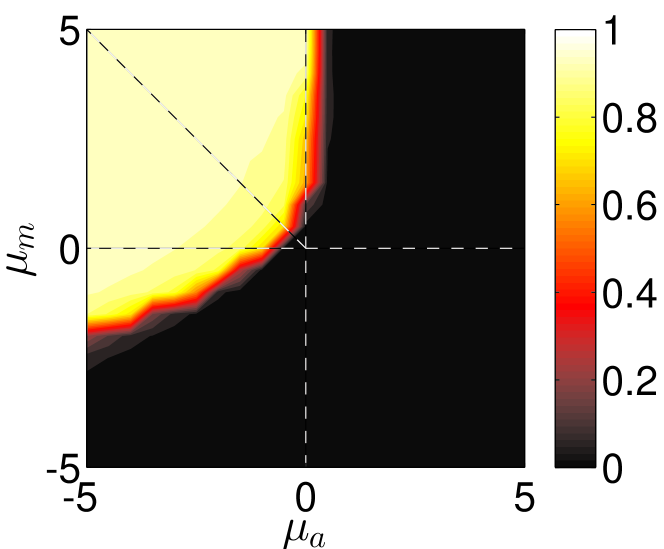 neighbor number
,
center of mass speed 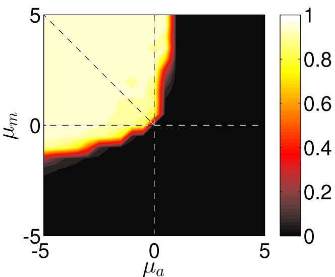 neighbor number
  ,
,
center of mass speed 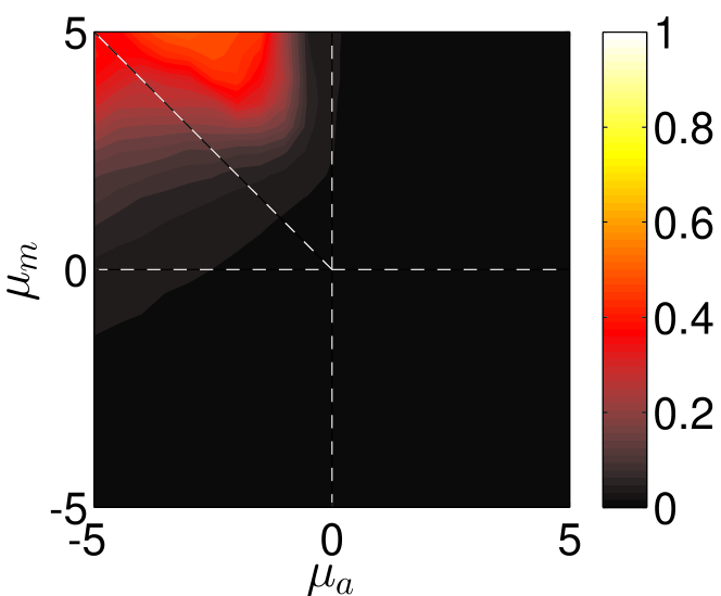 neighbor number
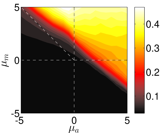
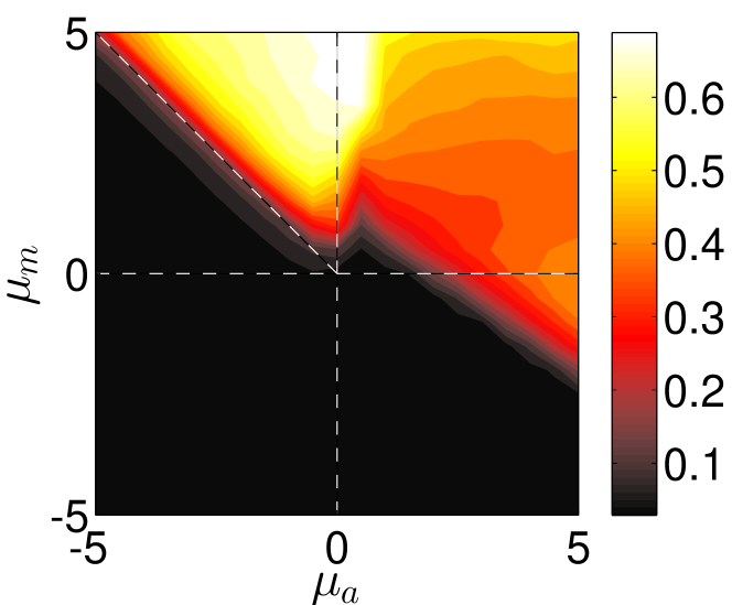
Throughout this work we set , and . Furthermore, we use , which ensures that for binary interactions the short-ranged repulsion is always larger than the sum of the other possibly attracting forces. The particle number is set constant to and the density is varied by changing the system size . The parameter-space diagrams in Figs. 4 and 5 were obtained from interpolating the results for and for () individual, evenly spaced, grid points in the interaction parameter space with . Each such point corresponds to an average over the results of 6 independent simulation runs, whereby for each run a temporal average was taken after the system reached a steady-state.
At sufficiently high densities and sufficiently low (angular) noise, we can observe the onset of collective motion for a wide range of interaction parameters (see Figs. 4 and 5). At low noise and high density, the region of collective motion coincides approximately with the escape and pursuit quadrant of the interaction parameter space with and . It contains the special cases of only attraction to moving away (repulsion from approaching) individuals with and ( and ), and extends also into the pure repulsion region ( and ) and to a much lesser extent into the pure attraction region ( and ). This is agreement with the predictions of the kinetic theory for the monopole approximation the effective social interaction. However, the region of collective motion is smaller in simulations than in the simple theory. This may be due to the impact of density inhomogeneities, finite short-range repulsion, and/or higher order effects.
Within the escape and pursuit regime, where the repulsion to approaching individuals (escape) dominates over the attraction to moving away individuals (pursuit), the neighbor number is low. This corresponds to low degree of clustering and a rather homogeneous spatial distribution of particles throughout the system. The neighbor number increases strongly in the pursuit dominated regime ( with , ) indicating strong density inhomogeneities corresponding to dense collectively moving bands and clusters. This resembles the behavior observed in the original Brownian particle escape & pursuit model.
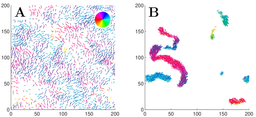
The neighbor number is also high in the pure attraction regime () without collective motion, where clusters with vanishing center of mass velocity can be observed. Interestingly, at moderate densities (, in Figs. 4,5), the maximum of the neighbor number is located in the pursuit-dominated regime with collective motion, and not, as one might expect, in the regime of (strong) overall attraction (). In the ordered state, particles move approximately in the same direction and the relative speed will be close to zero. For low repulsion from approaching individuals the escape response is negligible, whereas the attraction to moving away individual suffices to maintain cohesion, in particular at low noise strengths. Effectively, the density of such collectively moving cluster is limited by the short-range repulsion (see Fig. 6B). In the pure attraction regime, particles on the boundaries of a cluster will be attracted towards the local center of mass. However, due to the self-propelled motion with inertia and scattering with other individuals within the disordered cluster they will eventually move outwards again. As a result we observe disordered aggregates, which resemble mosquito swarms (see Fig. 2B), and are more dilute in comparison to the coherently moving clusters in the pursuit-dominated case.
As might be expected, increased stochasticity in the motion of individuals, inhibits the onset of collective motion. The region of parameter space with significantly larger than reduces strongly with increasing by receding towards the regime of strong escape and pursuit response (see Fig 5) in agreement with the kinetic theory.
For the Head-on-Head regime as well as for pure repulsion (with ) a quasi homogeneous distribution of particles can be observed with no collective motion (see Figs. 2C,D and 4,5 ).
V Discussion
In this work, we have analyzed a model for collective dynamics based on selective attraction and repulsion interactions, which was recently used to model the evolution of phenotypic phase change in locusts Guttal et al. (2012). The modelling of individual dynamics in terms stochastic differential equation (Langevin equations), allows a straight forward derivation of a kinetic description, which may be used for further theoretical analysis based on mean-field considerations and moment expansion of the corresponding probability density function Romanczuk and Schimansky-Geier (2011); Grossmann et al. (2012).
The model is able to account for three types of social responses relevant in the biological context: escape and pursuit, pure avoidance and pure attraction behavior. We have shown that large-scale collective motion of self-propelled particles emerge without any explicit velocity-alignment mechanism in the (generalized) escape and pursuit regime, without the spatial anisotropy in the social interaction in the original escape and pursuit model Romanczuk et al. (2009). Here, we should note that in the original escape-pursuit model, with Brownian dynamics of individual agents, the spatial anisotropy is essential for the emergence of directed collective motion.
In general, the spatial distribution of individuals during collective motion depends strongly on the relative strength of the different social forces. If escape dominates we observe a homogeneous spatial distribution (Fig. 6A), whereas in the pursuit-dominated case compact, coherently moving structures, as for example snake-like clusters, can be observed (Fig. 6B). In between, for comparable escape and pursuit strengths the band like structures perpendicular to the average direction of motion emerge, which appear also in systems with velocity-alignment (Fig. 2A) Grégoire and Chaté (2004); Romanczuk et al. (2012).
The region of collective motion decreases with increasing noise as well as with decreasing density. However, at low densities, the region of collective motion shows a clear shift towards the pursuit-dominated regime (see Fig 4 top), where in a finite system a order parameter is maintained by relatively few moving clusters containing most of the individuals.
These results are not only in agreement with the basic, qualitative predictions, drawn from the kinetic theory in Sect. III, but resemble also the qualitative behavior of the original escape-pursuit model Romanczuk et al. (2009). Interestingly, at intermediate densities and within the interaction range studied, the maximum of the neighbor number – indicating strongest clustering in the system – appears in the pursuit-dominated regime and not for pure attraction. This can be understood from the fact that local order decreases the effective “temperature” associated with absolute deviations of the velocities of single particles from the average velocity of their neighborsRomanczuk and Erdmann (2010); Romanczuk and Schimansky-Geier (2011). As a result we observe a decrease in the active pressure due to the stochastic self-propelled nature of individual motion, which counteracts the concentration of individuals due to attractive forces.
In conclusion, the modelling of collective motion in biology via selective attraction-repulsion interactions appears very promising. The model accounts for various individual behaviors and displays different spatial patterns of collective motion. The response based only on the distinction between approaching and moving away individuals can be directly linked to the response to looming visual stimuli, which has been shown to play an important role in various species Schiff et al. (1962); Rind and Simmons (1992, 1992, 1992); de Vries and Clandinin (2012). Finally, in this context, we should mention a recent work by Lemasson and coworkers Lemasson et al. (2009). They introduce a model for collective motion based on selective interaction of individuals based on explicit, simplified description of visual information available to each individual.
Acknowledgment
PR would like to thank Vishwesha Guttal (Indian Institute of Science) and Iain D. Couzin (Princeton University) for many helpful discussions on the subject. Part of the work was performed during a stay of LSG at IFISC in Palma de Mallorca. LSG thanks for the great hospitality and the fruitful cooperation. Furthermore, LSG acknowledges the support by the DFG via the IRTG 1740.
References
- Couzin et al. (2002) I. D. Couzin, J. Krause, R. James, G. D. Ruxton, and N. R. Franks, Journal of Theoretical Biology, 218, 1 (2002).
- Krause and Ruxton (2002) J. Krause and G. D. Ruxton, Living in groups (Oxford University Press, 2002) ISBN 9780198508182.
- Yates et al. (2009) C. A. Yates, R. Erban, C. Escudero, I. D. Couzin, J. Buhl, I. G. Kevrekidis, P. K. Maini, and D. J. T. Sumpter, Proceedings of the National Academy of Sciences, 106, 5464 (2009).
- Bazazi et al. (2011) S. Bazazi, P. Romanczuk, S. Thomas, L. Schimansky-Geier, J. J. Hale, G. A. Miller, G. A. Sword, S. J. Simpson, and I. D. Couzin, Proceedings of the Royal Society B: Biological Sciences, 278, 356 (2011).
- Vicsek et al. (1995) T. Vicsek, A. Czirók, E. Ben-Jacob, I. Cohen, and O. Shochet, Physical Review Letters, 75, 1226 (1995).
- Toner and Tu (1995) J. Toner and Y. Tu, Physical Review Letters, 75, 4326 (1995).
- Toner and Tu (1998) J. Toner and Y. Tu, Physical Review E, 58, 4828 (1998).
- Grégoire and Chaté (2004) G. Grégoire and H. Chaté, Physical Review Letters, 92, 025702 (2004).
- Aldana et al. (2007) M. Aldana, V. Dossetti, C. Huepe, V. M. Kenkre, and H. Larralde, Physical Review Letters, 98, 095702 (2007).
- Chaté et al. (2008) H. Chaté, F. Ginelli, G. Grégoire, and F. Raynaud, Physical Review E, 77, 046113 (2008).
- Romanczuk et al. (2009) P. Romanczuk, I. D. Couzin, and L. Schimansky-Geier, Physical Review Letters, 102, 010602 (2009).
- Romanczuk et al. (2012) P. Romanczuk, M. Bär, W. Ebeling, B. Lindner, and L. Schimansky-Geier, The European Physical Journal Special Topics, 202, 1 (2012), ISSN 1951-6355, 1951-6401.
- Leonard et al. (2007) N. Leonard, D. Paley, F. Lekien, R. Sepulchre, D. Fratantoni, and R. Davis, Proceedings of the IEEE, 95, 48 (2007), ISSN 0018-9219.
- Sepulchre et al. (2008) R. Sepulchre, D. Paley, and N. Leonard, Automatic Control, IEEE Transactions on, 53, 706 (2008), ISSN 0018-9286.
- Turgut et al. (2008) A. Turgut, H. Çelikkanat, F. Gökçe, and E. Şahin, Swarm Intelligence, 2, 97 (2008), ISSN 1935-3812.
- Ferrante et al. (2011) E. Ferrante, A. Turgut, N. Mathews, M. Birattari, and M. Dorigo, in Parallel Problem Solving from Nature – PPSN XI, Lecture Notes in Computer Science, Vol. 6239, edited by R. Schaefer, C. Cotta, J. Kolodziej, and G. Rudolph (Springer Berlin / Heidelberg, 2011) pp. 331–340, ISBN 978-3-642-15870-4.
- Cucker and Smale (2007) F. Cucker and S. Smale, Automatic Control, IEEE Transactions on, 52, 852 (2007), ISSN 0018-9286.
- Carrillo et al. (2010) J. A. Carrillo, M. Fornasier, G. Toscani, and F. Vecil, in Mathematical Modeling of Collective Behavior in Socio-Economic and Life Sciences, Modeling and Simulation in Science, Engineering and Technology, edited by G. Naldi, L. Pareschi, G. Toscani, and N. Bellomo (Birkhäuser Boston, 2010) pp. 297–336, ISBN 978-0-8176-4946-3.
- Niwa (1994) H. Niwa, Journal of Theoretical Biology, 171, 123 (1994), ISSN 0022-5193.
- Couzin et al. (2005) I. D. Couzin, J. Krause, N. R. Franks, and S. A. Levin, Nature, 433, 513 (2005).
- Romanczuk et al. (2008) P. Romanczuk, U. Erdmann, H. Engel, and L. Schimansky-Geier, The European Physical Journal Special Topics, 157, 61 (2008), ISSN 1951-6355.
- Bode et al. (2010) N. W. F. Bode, D. W. Franks, and J. A. Wood, Journal of Theoretical Biology, 267, 292 (2010), ISSN 0022-5193.
- Herbert-Read et al. (2011) J. E. Herbert-Read, A. Perna, R. P. Mann, T. M. Schaerf, D. J. T. Sumpter, and A. J. W. Ward, Proceedings of the National Academy of Sciences (2011), doi:10.1073/pnas.1109355108.
- Katz et al. (2011) Y. Katz, K. Tunstrøm, C. C. Ioannou, C. Huepe, and I. D. Couzin, Proceedings of the National Academy of Sciences (2011), doi:10.1073/pnas.1107583108.
- Ebeling and Schweitzer (2001) W. Ebeling and F. Schweitzer, Theory in Biosciences, 120, 207–224 (2001), ISSN 1431-7613.
- Peruani et al. (2006) F. Peruani, A. Deutsch, and M. Bär, Physical Review E (Statistical, Nonlinear, and Soft Matter Physics), 74, 030904 (2006).
- Grossman et al. (2008) D. Grossman, I. S. Aranson, and E. B. Jacob, New Journal of Physics, 10, 023036 (2008).
- Strefler et al. (2008) J. Strefler, U. Erdmann, and L. Schimansky-Geier, Physical Review E, 78, 031927 (2008).
- Strömbom (2011) D. Strömbom, Journal of Theoretical Biology, 283, 145 (2011), ISSN 0022-5193.
- Simpson et al. (2006) S. J. Simpson, G. A. Sword, P. D. Lorch, and I. D. Couzin, PNAS, 103, 4152 (2006).
- Bazazi et al. (2008) S. Bazazi, J. Buhl, J. J. Hale, M. L. Anstey, G. A. Sword, S. J. Simpson, and I. D. Couzin, Current Biology, 18, 735 (2008), ISSN 0960-9822.
- Guttal et al. (2012) V. Guttal, P. Romanczuk, S. J. Simpson, G. A. Sword, and I. D. Couzin, submitted (2012).
- Couzin et al. (2011) I. D. Couzin, C. C. Ioannou, G. Demirel, T. Gross, C. J. Torney, A. Hartnett, L. Conradt, S. A. Levin, and N. E. Leonard, Science, 334, 1578 (2011), ISSN 0036-8075, 1095-9203.
- Romanczuk and Erdmann (2010) P. Romanczuk and U. Erdmann, The European Physical Journal Special Topics, 187, 127 (2010), ISSN 1951-6355.
- Romanczuk and Schimansky-Geier (2011) P. Romanczuk and L. Schimansky-Geier, Ecological Complexity (2011), ISSN 1476-945X, doi:10.1016/j.ecocom.2011.07.008.
- Grossmann et al. (2012) R. Grossmann, L. Schimansky-Geier, and P. Romanczuk, arXiv:1204.4304 (2012).
- Schiff et al. (1962) W. Schiff, J. A. Caviness, and J. J. Gibson, Science, 136, 982 (1962), ISSN 0036-8075, 1095-9203.
- Rind and Simmons (1992) F. C. Rind and P. J. Simmons, J Neurophysiol, 68, 1654 (1992).
- de Vries and Clandinin (2012) S. de Vries and T. Clandinin, Current Biology, 22, 353 (2012), ISSN 0960-9822.
- Lemasson et al. (2009) B. Lemasson, J. Anderson, and R. Goodwin, Journal of Theoretical Biology, 261, 501 (2009), ISSN 0022-5193.