Scale dependent halo bias in the excursion set approach

Abstract

If one accounts for correlations between scales, then nonlocal, $k$-dependent halo bias is part and parcel of the excursion set approach, and hence of halo model predictions for galaxy bias. We present an analysis that distinguishes between a number of different effects, each one of which contributes to scale-dependent bias in real space. We show how to isolate these effects and remove the scale dependence, order by order, by cross-correlating the halo field with suitably transformed versions of the mass field. These transformations may be thought of as simple one-point, two-scale measurements that allow one to estimate quantities which are usually constrained using $n$-point statistics. As part of our analysis, we present a simple analytic approximation for the first crossing distribution of walks with correlated steps which are constrained to pass through a specified point, and demonstrate its accuracy. Although we concentrate on nonlinear, nonlocal bias with respect to a Gaussian random field, we show how to generalize our analysis to more general fields.

1 Introduction

Galaxy clustering depends on galaxy type (Zehavi et al. 2011 and references therein). Therefore, not all galaxies are fair tracers of the dark matter distribution. Precise constraints on cosmological models require a good understanding of this galaxy bias (Sefusatti et al. 2006; More et al. 2012). In the simplest models, galaxies are linearly biased tracers (Kaiser 1984), but, even at the linear level, this bias may depend on physical scale or wavenumber $k$ (e.g. Desjacques et al. 2010; Matsubara 2011). This scale-dependence, which is clearly detected in simulations of hierarchical clustering models (Sheth & Tormen 1999; Smith et al. 2007; Manera et al. 2010), contains important information about the statistics of the initial fluctuation field, and the nature of gravity (Parfrey, Hui & Sheth 2011; Lam & Li 2012).

The most common galaxy bias model – the local bias model – assumes that the galaxy overdensity field $\delta_{h}(x)$ is a local, possibly nonlinear, monotonic, deterministic transformation of the dark matter field $\delta(x)$ at the same position (Fry & Gaztañaga 1993; Manera & Gaztañaga 2012; Pollack, Smith & Porciani 2012; Chan & Scoccimarro 2012). Even in this case, there are a number of ways in which scale dependence can arise, even for the simplest case of Gaussian initial conditions and standard gravity. Since the measured bias will generally be a combination of all these effects, we present some ideas on how to disentagle them from one another.

In general, of course, $\delta_{h}$ might depend on the value of $\delta$ at different locations, on its derivatives (Desjacques et al. 2010; Musso & Sheth 2012), on other higher order statistics of the field (e.g. Sheth, Mo & Tormen 2001; Sheth, Chan & Scoccimarro 2012) at the same or at different positions, etc.; the dependence might even not be deterministic (e.g., Sheth & Lemson 1999; Dekel & Lahav 1999). Our final goal is to present methods which are able to pinpoint this relation even when the bias is nonlinear, nonlocal and stochastic.

We study insights which arise from the simplest treatment of halo bias: that based on the excursion set approach (Press & Schechter 1974). This approach maps the problem of counting the number of collapsed halos to that of the first crossing of a suitable threshold (the ‘barrier’) by random walks in density generated by smoothing the initial matter density field using a sequence of filters of decreasing scales (Bond et al. 1991). In addition to depending on the ‘barrier’ shape, the first crossing distribution also depends on how far from the ‘origin’ the walks happen to be for the largest smoothing scale $S_{0}$.

Walks that do not start from the origin have modified first crossing distributions (Lacey & Cole 1993). This introduces a dependence of the abundance of halos $1+\delta_{h}$ on the initial matter density field $\delta$ smoothed on the much larger scale $S_{0}$, and hence leads to a prediction for halo bias (Mo & White 1996).

The excursion set approach greatly simplifies when the smoothing filter is sharp in Fourier space, because in this case the steps in each walk are uncorrelated with each other. Since most analyses to date have relied on this choice, we use it to illustrate many of our key points. E.g., if the bias is deterministic and nonlinear in real-space, it will be stochastic in $k$-space. And, estimates of cross-correlations between the halo and mass fields depend on the assumed form of the probability distribution function of the mass: one must be careful to use the appropriate probability density function (pdf). One of the key insights of this paper is to show that suitably defined real-space cross-correlation measurements allow one to extract the different bias coefficients, order by order.

Recently, however, there has been renewed interest in studying the effects of smoothing with more realistic filters such as the TopHat in real space or the Gaussian. The problem is complicated in this case by the presence of nontrivial correlations between the steps of the random walks (Peacock & Heavens 1990; Bond et al. 1991), and a number of different approximations for the effect on the first crossing distribution have been introduced (Maggiore & Riotto 2010; Paranjape, Lam & Sheth 2012). We show that the most accurate of these, due to Musso & Sheth (2012), can be extended to provide a very accurate model for walks which do not start from the origin.

We then show that correlations between steps generically introduce two additional sources of scale-dependent bias into the predictions. One is relatively benign, and simply arises from the fact that the excursion set prediction is for a real-space quantity, but the halo bias in $N$-body simulations is typically measured in Fourier space, through ratios of power spectra. That this matters reiterates a point first made by Paranjape & Sheth (2012), but it is easily accounted for by using a more appropriate normalization of the bias coefficients. The second is more pernicious and is a genuinely new source of $k$-dependent bias (a point made in Musso & Sheth 2012, but not studied further). Although this complicates discussion of scale-dependent bias, our method of measuring suitably defined real-space cross-correlations between the halo and mass fields can be used to extract the $k$-dependence of halo bias order by order.

This paper is organised as follows. Section 2 briefly summarizes known excursion set results for uncorrelated steps, defines the halo bias factors as a ratio of real space measurements, derives their large scale limiting values, uses these to motivate a real-space cross-correlation measurement at finite scale which returns these limiting values, and quantifies the importance of computing averages over the correct ensemble.

Section 3 extends these results to the case of correlated steps. We first derive the conditional distribution $f(s|\delta_{0},S_{0})$ that a walk crosses the barrier for the first time at scale $s$ having taken up the value $\delta_{0}$ at scale $S_{0}$, and demonstrate its accuracy by comparing with the results of a Monte Carlo treatment of the problem. We then turn to the problem of halo bias, and highlight some important differences from the uncorrelated case: the question of the correct pdf is shown to be much less important, whereas the scale dependence of bias becomes more dramatic. We discuss some of the implications of our analysis and conclude in section 4. Appendix A collects proofs of some results quoted in the text, while Appendix B connects the bias coefficients defined using cross-correlation measurements to other definitions in the literature.

Throughout we will present results for a constant barrier of height $\delta_{\rm c}$. Moving barriers pose no conceptual difficulty for the first crossing distributions we are interested in. Also, while our analytical results are generally valid for any smoothing filter and power spectrum, for ease of implementation, the explicit comparisons with numerical solutions will use the Gaussian filter and a power law power spectrum. Again, we do not expect our final conclusions to depend on this choice.

2 The excursion set approach: Uncorrelated steps

The excursion set ansatz relates the number of halos in a mass range $(m,m+{\rm d}m)$ to the fraction $f(s)$ of walks that first cross the barrier in the scale range $(s,s+{\rm d}s)$ through the relation

$$\frac{m}{\bar{\rho}}\frac{{\rm d}n(m)}{{\rm d}m}{\rm d}m=f(s)\,{\rm d}s,$$ (1)

where $s=s(m)\equiv\left\langle\,\delta^{2}(m)\,\right\rangle$ is the variance of the matter density field smoothed on a Lagrangian length scale corresponding to mass $m$ and linearly extrapolated to present day, and $\bar{\rho}$ is the background density.

In this approach, the influence of the underlying dark matter field on the abundance of halos of mass $m$ (i.e. the bias) can be estimated from the fraction $f(s|\delta_{0},S_{0})$ of walks that first cross the barrier at $s$ starting from some prescribed height $\delta_{0}$ on some prescribed scale $S_{0}$, rather than from the origin (Mo & White 1996; Sheth & Tormen 1999). The mean number overdensity of halos can be defined as

$$\left\langle\,1+\delta_{\rm h}|\delta_{0},S_{0}\,\right\rangle\equiv\frac{f(s|\delta_{0},S_{0})}{f(s)}\,,$$ (2)

which is explicitly a prediction in real space, and valid on scale $S_{0}$ in the Lagrangian initial conditions.

Typically, the bias is characterised by expanding the above expression in powers of $\delta_{0}$. The coefficients of this expansion will in general depend on $S_{0}$ (besides obviously depending on $s$). Moreover, the evaluation of $f(s)$ and $f(s|\delta_{0},S_{0})$ (and therefore of the bias coefficients) is rather different depending on whether or not the steps in the walk are correlated. In what follows, we elucidate the issue of the scale dependence of the bias coefficients in the simpler case of walks with uncorrelated steps. We also argue that the same coefficients can be obtained as the mean value of the product of $\left\langle\,1+\delta_{\rm h}|\delta_{0},S_{0}\,\right\rangle$ and polynomials in $\delta_{0}$, weighted by the probability distribution of $\delta_{0}$. This alternative definition as an expectation value will be more suitable to be extended to the case of correlated steps (section 3), and to make contact with the definition of bias in generic models other than the excursion set approach (Appendix B).

2.1 Large scale Lagrangian bias factors

The conditional first crossing distribution of a constant barrier $\delta_{\rm c}$ for walks with uncorrelated steps is (Bond et al. 1991; Lacey & Cole 1993)

$$f_{\rm u}(s|\delta_{0},S_{0})=\frac{1}{\sqrt{2\pi}}\frac{\delta_{\rm c}-\delta_{0}}{(s-S_{0})^{3/2}}{\rm e}^{-(\delta_{\rm c}-\delta_{0})^{2}/2(s-S_{0})}\,,$$ (3)

(the subscript in $f_{\rm u}$ standing for “uncorrelated”), where $\delta_{\rm c}>\delta_{0}$ and $s>S_{0}$. The corresponding unconditional distribution is $sf_{\rm u}(s)=(2\pi)^{-1/2}\nu{\rm e}^{-\nu^{2}/2}$, where $\nu^{2}\equiv\delta_{\rm c}^{2}/s$. In this case, setting $S_{0}=0$ and expanding around $\delta_{0}=0$ leads to (Mo & White 1996; Mo, Jing & White 1997)

$$\frac{f_{\rm u}(s|\delta_{0},S_{0}=0)}{f_{\rm u}(s)}=1+\sum_{n=1}^{\infty}\frac{\delta_{0}^{n}}{n!}b^{\rm u}_{n}(\nu)\,,$$ (4)

with the bias coefficients given by

$$\delta_{\rm c}^{n}b^{\rm u}_{n}=\nu^{n-1}H_{n+1}(\nu)\,,$$ (5)

where $H_{m}(x)={\rm e}^{x^{2}/2}(-d/dx)^{m}{\rm e}^{-x^{2}/2}$ are the “probabilist’s” Hermite polynomials. For example, $n=1$ returns the familiar expression for the linear halo bias $b^{\rm u}_{1}=(\nu^{2}-1)/\delta_{\rm c}$. Note that these coefficients are pure numbers, independent of wavenumber $k$, and (by definition) of $S_{0}$. It is these scale-independent numbers which are most often used to derive cosmological constraints. (Of course, for non-negligible $S_{0}$, the Taylor series expansion of equation (2) will yield bias coefficients that depend on $S_{0}$, but this dependence is almost never calculated or used.) Since the $S_{0}\to 0$ limit of equation (3) corresponds to setting $\delta_{\rm c}\to\delta_{\rm c}-\delta_{0}$ in the unconditional crossing distribution, these $b_{n}$ are simply related to the $n$th derivative of $sf_{\rm u}(s)$ with respect to $\delta_{\rm c}$. This makes it easy to see why the Hermite polynomials feature so prominently in much of what follows.

2.2 A weighted-average definition of bias

If we ignore the fact that the conditional distribution in equation (3) should really have $\delta_{0}<\delta_{\rm c}$, then it is easy to check that

$$f_{\rm u}(s)=\int_{-\infty}^{\infty}{\rm d}\delta_{0}\,f_{\rm u}(s|\delta_{0},S_{0})\,p_{\rm G}(\delta_{0};S_{0}).$$ (6)

where $p_{\rm G}(\delta_{0};S_{0})$ is a Gaussian distribution with zero mean and variance $S_{0}$. Although this result is formally correct, we argue in the next subsection that the appropriate distribution over which to average should not be a Gaussian (nor even a Gaussian chopped at $\delta_{0}>\delta_{\rm c}$). But if we continue to ignore this detail, then we find

$$\int_{-\infty}^{\infty}{\rm d}\delta_{0}\,p_{\rm G}(\delta_{0};S_{0})\frac{f_{\rm u}(s|\delta_{0},S_{0})}{f_{\rm u}(s)}\delta_{0}\,=b^{\rm u}_{1}\,S_{0}$$

(Desjacques et al. 2010), and more generally, the orthogonality of the Hermite polynomials implies (Appendix A.1) that

$$\frac{\delta_{\rm c}^{n}}{S_{0}^{n/2}}\left\langle\,\frac{f_{\rm u}(s|\delta_{0},S_{0})}{f_{\rm u}(s)}\,H_{n}\left(\frac{\delta_{0}}{\sqrt{S_{0}}}\right)\,\right\rangle=\delta_{\rm c}^{n}b^{\rm u}_{n}.$$ (7)

This exact result is remarkable because the left hand side involves quantities for an arbitrary $S_{0}$, whereas the right hand side, which is independent of $S_{0}$, is simply the $S_{0}\to 0$ limit of the appropriate bias coefficient. This is not at all obvious if one had viewed the local bias expansion as a formal Taylor series: one would naively have thought that, at the very least, the cross correlation $\left\langle\,(1+\delta_{\rm h})\delta_{0}\,\right\rangle$ should involve the bias coefficients of all (odd) orders (for a further discussion, see Frusciante & Sheth 2012).

Strictly speaking, this is only a mathematical curiousity, since the conditional distribution $f_{\rm u}(s|\delta_{0},S_{0})$ is formally zero for $\delta_{0}>\delta_{\rm c}$, but the identity above holds only when (incorrectly) averaging the expression in (3) over the full (Gaussian) distribution of $\delta_{0}$. However, if we forget for the moment about how the bias factors in equation (5) were determined, then the analysis above shows that the $S_{0}\to 0$ limit of the bias coefficients can be recovered by cross-correlating the halo overdensity field with a suitably transformed version of the mass field (the transformation uses Hermite polynomials). In particular, our cross-correlation method works for any smoothing scale $S_{0}$; there is no requirement that this scale be large (although, strictly speaking, one does require that $S_{0}<s$, i.e., that the smoothing scale be larger than that used for defining the halos in the first place).

There are two important lessons here. First, treating the $S_{0}\to 0$ limit of the bias coefficients as though they are arbitrary is risky: one must be careful to ensure that the implied conditional distribution function is sensible (e.g. positive definite). Except for the coefficients which come from the more physically motivated excursion set approach, this is rarely ever done. We return to this point in the next subsection. The second lesson is that cross-correlating with appropriate transformations of the mass field may be an efficient way of isolating the different large scale bias coefficients from one another. One view of this second lesson is to contrast it with the usual probe of higher order bias factors: 2-point statistics constrain $b_{1}$, 3-point statistics constraint both $b_{1}$ and $b_{2}$, and so on (Sefusatti & Scoccimarro 2005; Smith et al. 2007; Pollack et al. 2012). Since the Hermite polynomials here are polynomials, one may think of the transformation as picking out that combination of $n$-point functions which isolates the dependence on $b_{n}$. The analysis above suggests that, once the appropriate transformation has been made, $b_{n}$ can be determined by a real-space cross-correlation measurement alone, and this cross-correlation be made on any smoothing scale $S_{0}$; there is no requirement that this scale be large.

2.3 Scale dependence from appropriate averaging

The previous subsection noted that a naive averaging of $\left\langle\,1+\delta_{\rm h}|\delta_{0}\,\right\rangle$ over a Gaussian distribution appeared to return the large-scale $S_{0}\to 0$ bias factors. However, the correct distribution over which to average is not a Gaussian, but

$$q_{\rm u}(\delta_{0},S_{0};\delta_{\rm c})=\frac{1}{\sqrt{2\pi S_{0}}}\left[{\rm e}^{-\delta_{0}^{2}/2S_{0}}-{\rm e}^{-(2\delta_{\rm c}-\delta_{0})^{2}/2S_{0}}\right]\,,$$ (8)

where $\delta_{0}<\delta_{\rm c}$ (Sheth & Lemson 1999). This is because $q_{\rm u}(\delta_{0},S_{0};\delta_{\rm c})$ gives the probability that the walk had height $\delta_{0}$ at scale $S_{0}$, and remained below the barrier $\delta_{\rm c}$ on all scales $S<S_{0}$ (Chandrasekhar 1943). It is easy to check that

$$f_{\rm u}(s)=\int_{-\infty}^{\delta_{\rm c}}{\rm d}\delta_{0}\,f_{\rm u}(s|\delta_{0},S_{0})\,q_{\rm u}(\delta_{0},S_{0};\delta_{\rm c})\,,$$ (9)

as it should.

For similar reasons, whenever one deals with the conditional mean $\left\langle\,1+\delta_{\rm h}|\delta_{0}\,\right\rangle$, the appropriate way to compute cross correlations between the halo overdensity field and the mass is by averaging over $q$ and not $p$, and this generically makes the measured coefficients depend on scale $S_{0}$ as we discuss below. For $n=1$, this yields

$$\frac{\delta_{\rm c}}{S_{0}}\left\langle\,\delta_{0}\left\langle\,1+\delta_{h}|\delta_{0}\,\right\rangle\,\right\rangle_{q} =H_{2}(\nu)+(\nu_{10}^{2}+1){\rm erfc}\left(\nu_{10}/\sqrt{2}\right)$$

$$\phantom{H_{2}(\nu)}\qquad-\sqrt{2\nu_{10}^{2}/\pi}\,e^{-\nu_{10}^{2}/2}$$ (10)

where $\nu_{10}^{2}=\nu^{2}\,(s/S_{0}-1)$ (equation 17 in Sheth & Lemson 1999). Note that, in contrast to the previous calculation, this quantity yields $H_{2}(\nu)$ only in the limit $S_{0}\to 0$. Similarly, averaging $(1+\delta_{\rm h})H_{n}$ over $q_{\rm u}$ yields a more complicated function of $S_{0}$.

Figure 1: Monte-Carlo measurement of the cross-correlation between $\delta_{\rm h}$ and $\delta_{0}$ (top) and $H_{2}$ (bottom), for walks with uncorrelated steps. See the main text for a description of the measurement. Solid curves show the prediction associated with averaging over a Gaussian distribution, as is commonly done, and which the main text argued was inappropriate, and dashed curves show the result of averaging using $q$ of equation (8).

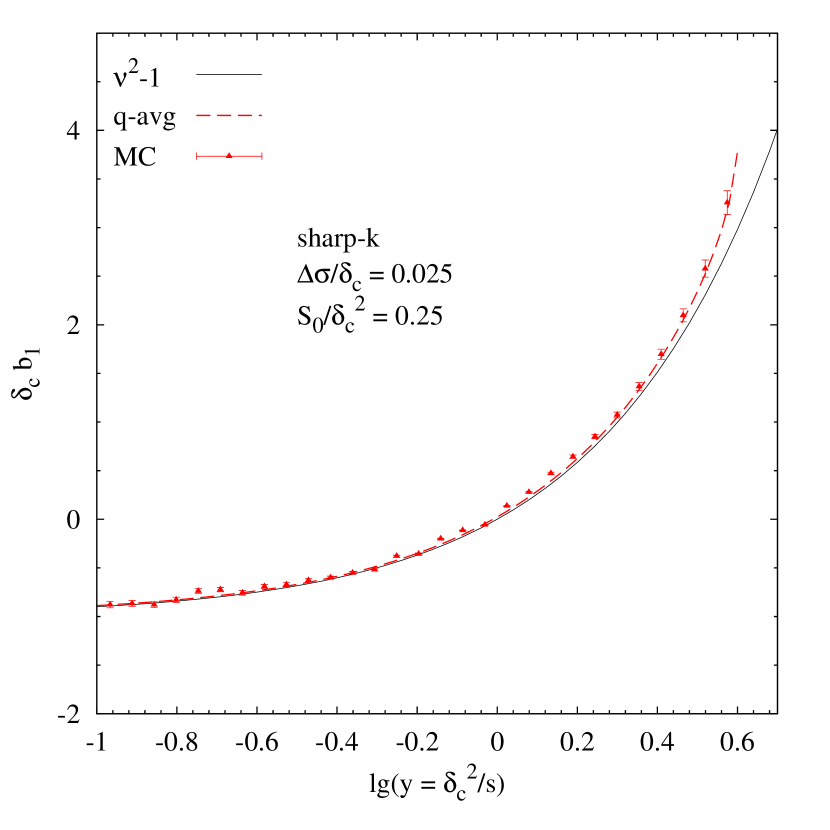
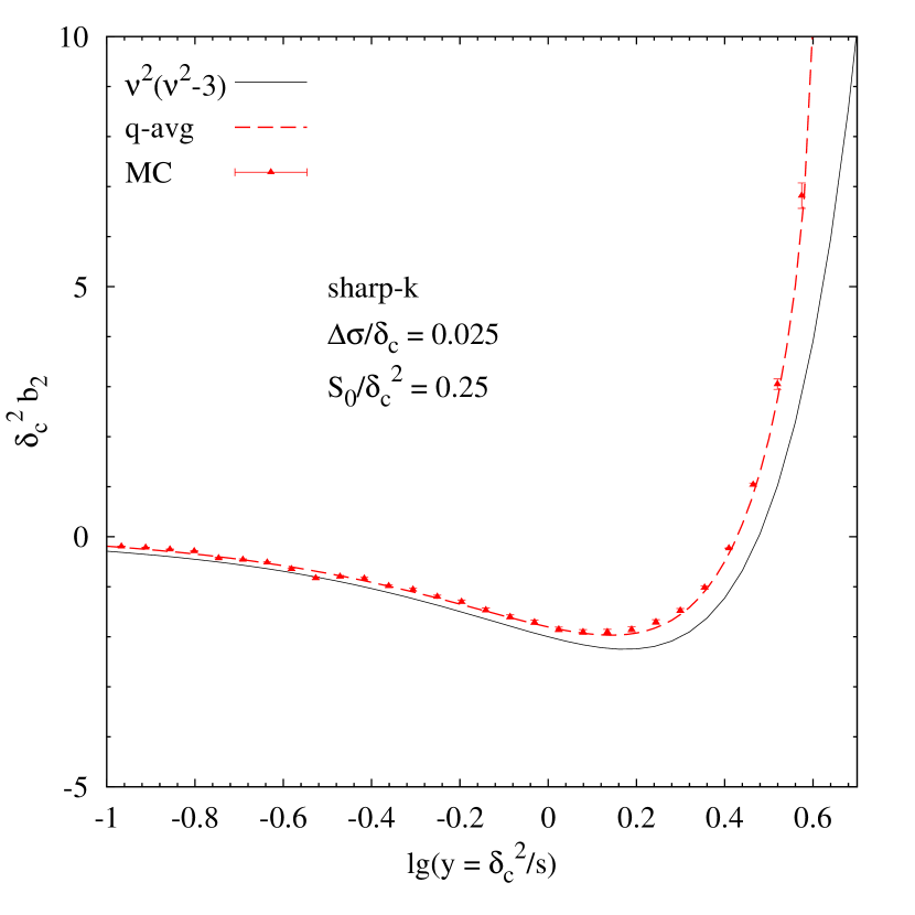
We have verified these analytical arguments in a comparison with numerical results. The symbols in Figure 1 show a measurement of the cross-correlation between $\delta_{0}$ and $(1+\delta_{\rm h})$ in a Monte Carlo simulation of random walks with uncorrelated steps. We generate these walks by accumulating independent Gaussian draws, each with zero mean and variance $(\Delta\sigma)^{2}$. For each such walk, we note the scale $s$ at which it first crossed a constant barrier $\delta_{\rm c}$, as well as its height $\delta_{0}$ at a chosen scale $S_{0}$. The Figure shows results for $\Delta\sigma/\delta_{\rm c}=0.025$ and $S_{0}/\delta_{\rm c}^{2}=0.25$. To measure the correlation in a given bin in $y=\delta_{\rm c}^{2}/s$, we identify those walks that first cross $\delta_{\rm c}$ in this bin. If these are $N_{y}$ in number, we compute the mean $\sum_{j=1}^{N_{y}}H_{n}(\delta_{0j}/\sqrt{S_{0}})/N_{y}$ where $\delta_{0j}$ is the height at $S_{0}$ of the $j^{\rm th}$ such walk. Dividing this mean by $S_{0}^{n/2}$ gives the numerical estimate of $b_{n}$. Since the first-crossing of $\delta_{\rm c}$ for these walks is at $s>S_{0}$ by construction, this measurement is a $q$-averaged one.

The two panels show the measurements for $n=1$ and $2$, and the solid and dashed curves show the analytic result of averaging using $p$ and $q$, respectively. The solid curve remains the same for all $S_{0}$ (equation 7) but the dashed one does not (e.g. equation 10). Therefore, the difference between the solid and dashed predictions depends on $S_{0}$; we have checked that averaging over $q_{\rm u}$ always yields the correct, scale-dependent value.

While this agreement demonstrates that we have a good understanding of just what it is that the excursion set returns, and of the $S_{0}$ scale-dependence of the bias coefficients returned by a cross-correlation measurement – it has also shown that averaging equation (3) over a Gaussian distribution (rather than $q_{\rm u}$) will lead to incorrect estimates of the bias factors and their scale dependence.

The fact that $q\neq p$ leads to measureable differences suggests that unless one has a good model of how both $f$ and $q$ depend on scale, one must use large survey volumes (to ensure one is safely in the $S_{0}\to 0$ limit) if halo bias (e.g. equation 4) is to constrain parameters. At the moment, this understanding exists only for the special case of predictions based on walks with uncorrelated steps. Unfortunately, for the $q$-averaging which we have argued is the more appropriate, it is not straightforward to separate out the scale independent terms $H_{n}(\nu)$ from those which depend on $S_{0}$ (e.g., through $\nu_{10}$). If it were, we would be able to derive cosmological constraints from smaller volumes. As it stands, if walks with uncorrelated steps were a realistic model, then for halos with $\nu\sim 1.3$ (mass $m\sim 10^{13}h^{-1}M_{\odot}$ or Lagrangian scales $R\sim 3h^{-1}$Mpc), in order to achieve percent level accuracy in predicting the scale-independent $b_{1}$ ($b_{2}$), one would need to work at scales $S_{0}/\delta_{\rm c}^{2}\simeq 0.155$ ($0.115$) or Lagrangian scales $R_{0}\sim 10h^{-1}$Mpc ($14h^{-1}$Mpc). We now turn to a study of these issues for the more realistic case of walks with correlated steps.

3 The excursion set approach with correlated steps

We would like to extend the analysis of the previous section to include the effects of correlated steps. To do so, we must first set up some notation.

3.1 Notation

Let us recall some standard results regarding Gaussian distributions, which we will use frequently. If the joint distribution $p(x_{1},x_{2})$ for two variables is the bivariate Gaussian with zero mean, then

$$p(x_{1},x_{2}) =p_{\rm G}(\mathbf{x};\mathbf{C})\equiv\frac{{\rm e}^{-\frac{1}{2}\mathbf{x}^{\rm T}\mathbf{C}^{-1}\,\mathbf{x}}}{\sqrt{(2\pi)^{2}\mathrm{Det}[\mathbf{C}]}}\,,$$ (11)

where $\mathbf{C}$ is the covariance matrix $\mathbf{C}_{ij}=\left\langle\,x_{i}x_{j}\,\right\rangle$.

If the joint distribution $p(x_{1},x_{2},x_{3})$ for three variables is a trivariate Gaussian, then the conditional distribution $p(x_{1},x_{2}|x_{3})$ is also a bivariate Gaussian:

$$p(x_{1},x_{2}|x_{3}) =p_{\rm G}(\mathbf{x}-\bar{}\mathbf{x};\mathbf{C}-\tilde{}\mathbf{c})\,,$$ (12)

where the conditional mean $\bar{}\mathbf{x}$ is proportional to $x_{3}$,

$$\bar{}\mathbf{x} =x_{3}\bigg{(}\frac{\left\langle\,x_{1}x_{3}\,\right\rangle}{\left\langle\,x_{3}^{2}\,\right\rangle},\frac{\left\langle\,x_{2}x_{3}\,\right\rangle}{\left\langle\,x_{3}^{2}\,\right\rangle}\bigg{)}\,.$$ (13)

The “correction” to the covariance matrix $\tilde{}\mathbf{c}$ accounts for that part of the correlation between $x_{1}$ and $x_{2}$ which is due to a correlation with $x_{3}$. Its components are $\tilde{}\mathbf{c}_{11}=\left\langle\,x_{1}x_{3}\,\right\rangle^{2}/\left\langle\,x_{3}^{2}\,\right\rangle$, $\tilde{}\mathbf{c}_{22}=\left\langle\,x_{2}x_{3}\,\right\rangle^{2}/\left\langle\,x_{3}^{2}\,\right\rangle$ and $\tilde{}\mathbf{c}_{12}=\left\langle\,x_{1}x_{3}\,\right\rangle\left\langle\,x_{3}x_{2}\,\right\rangle/\left\langle\,x_{3}^{2}\,\right\rangle$.

In the excursion set framework one is interested in $p(\delta,\delta^{\prime})$ and $p(\delta,\delta^{\prime}|\delta_{0})$, where $\delta^{\prime}$ is the “curvature” of the walk at scale $s$, $\delta^{\prime}={\rm d}\delta/{\rm d}s$. Since all three quantities $\delta$, $\delta^{\prime}$ and $\delta_{0}$ are essentially linear combinations of the underlying Gaussian-distributed Fourier modes, both these distributions are also Gaussian. In this case $\left\langle\,\delta^{2}\,\right\rangle=s$, $\left\langle\,\delta\delta^{\prime}\,\right\rangle=(1/2)({\rm d}/{\rm d}s)\left\langle\,\delta^{2}\,\right\rangle=1/2$ and $\left\langle\,\delta_{0}^{2}\,\right\rangle=S_{0}$, and the relevant quantities read

$$\mathbf{C}=\left[\!\begin{array}[]{cc}s&1/2\\ 1/2&\left\langle\,\!\delta^{\prime 2}\!\,\right\rangle\end{array}\!\right],\quad\tilde{}\mathbf{c}=\frac{S_{\times}^{2}}{S_{0}^{2}}\frac{S_{0}}{s}\!\left[\!\begin{array}[]{cc}s&\epsilon_{\times}/2\\ \epsilon_{\times}/2&\epsilon_{\times}^{2}/4s\end{array}\!\right]$$ (14)

and

$$\bar{}\mathbf{x}=\delta_{0}\frac{S_{\times}}{S_{0}}\left(1,\frac{\epsilon_{\times}}{2s}\right)\,,$$ (15)

where

$$S_{\times}\equiv\left\langle\,\delta\delta_{0}\,\right\rangle\quad\textrm{and}\quad\epsilon_{\times}\equiv 2s\frac{\left\langle\,\delta^{\prime}\delta_{0}\,\right\rangle}{\left\langle\,\delta\delta_{0}\,\right\rangle}\,.$$ (16)

For a Gaussian filter, $W(kR)=\exp(-k^{2}R^{2}/2)$, one has $S_{\times}=\sigma_{0\times}^{2}$ and $\epsilon_{\times}=\sigma_{1\times}^{2}\sigma_{0}^{2}/\sigma_{0\times}^{2}\sigma_{1}^{2}$, where

$$\sigma_{j\times}^{2} =\int\frac{{\rm d}k}{k}\frac{k^{3}P(k)}{2\pi^{2}}k^{2j}W(kR)W(kR_{0})\,,$$ (17)

$$\sigma_{j}^{2} =\int\frac{{\rm d}k}{k}\frac{k^{3}P(k)}{2\pi^{2}}k^{2j}W^{2}(kR)\,.$$ (18)

If, in addition, $P(k)\propto k^{n}$, then

$$\frac{S_{\times}}{S_{0}} =2^{(n+3)/2}\left(1+\left(S_{0}/s\right)^{2/(n+3)}\right)^{-(n+3)/2}\,,$$ (19)

$$\epsilon_{\times} =2(S_{0}/s)\left(1+\left(S_{0}/s\right)^{2/(n+3)}\right)^{-1}\,.$$ (20)

We will also use the same notation $p_{\rm G}(z;\sigma^{2})$ to denote a one-dimensional Gaussian distribution when there is no scope for confusion.

3.2 The unconditional distribution

Although our goal is to write down the analogue of equation (3) for the first crossing distribution associated with walks which are conditioned to pass through $\delta_{0}$ on scale $S_{0}$, our first step is to write down the unconstrained distribution. As shown by Musso & Sheth (2012), for a constant barrier of height $\delta_{\rm c}$ the latter is well-approximated by

$$f(s)=\int_{0}^{\infty}{\rm d}\delta^{\prime}\delta^{\prime}p(\delta_{\rm c},\delta^{\prime})\,,$$ (21)

where $p(\delta_{\rm c},\delta^{\prime})$ is the bivariate Gaussian $p_{\rm G}(\delta_{\rm c},\delta^{\prime};\mathbf{C})$ with covariance matrix given in equation (14).

The integral in equation (21) can be performed analytically and leads to

$$sf(s)=\frac{\nu{\rm e}^{-\nu^{2}/2}}{2\,\sqrt{2\pi}}\bigg{[}\frac{1+{\rm erf}\left(\Gamma\nu/\sqrt{2}\right)}{2}+\frac{{\rm e}^{-\Gamma^{2}\nu^{2}/2}}{\sqrt{2\pi}\Gamma\nu}\bigg{]},$$ (22)

with

$$\Gamma^{2}\equiv\frac{\gamma^{2}}{(1-\gamma^{2})}\quad{\rm and}\quad\gamma^{2}\equiv\frac{\left\langle\,\delta\delta^{\prime}\!\,\right\rangle^{2}}{\left\langle\,\delta^{2}\,\right\rangle\!\left\langle\,\delta^{\prime 2}\!\,\right\rangle}\,.$$ (23)

(Equation 22 corrects a typo in equation 6 of the published version of Musso & Sheth 2012.) For later convenience, the same can also be written as

$$sf(s)=\frac{{\rm e}^{-\nu^{2}(1+\Gamma^{2})/2}}{(2\pi)(2\Gamma)}\left(1+A\right)\,,$$ (24)

where

$$A\equiv A(\nu)=\frac{1}{2}\left[1+{\rm erf}\left(\frac{\Gamma\nu}{\sqrt{2}}\right)\right]\sqrt{2\pi}\,\Gamma\nu\,{\rm e}^{\Gamma^{2}\nu^{2}/2}\,.$$ (25)

Musso & Sheth (2012) showed that this approximation (as well as its generalisation to moving barriers) works extremely well over a large range of scales for a range of choices of power spectra and filters (including TopHat filtered LCDM) when compared with Monte Carlo solutions of the first crossing problem. (It breaks down in the limit in which the walks must have taken many steps to cross the barrier.) Our final analytic results in this paper will be valid for arbitrary power spectra and filters for a constant barrier. However, since explicit expressions for various quantities greatly simplify for the choice of Gaussian smoothing of power law power spectra, we will show comparisons with Monte Carlo solutions for the latter. For Gaussian smoothing, $\gamma=\sigma_{1}^{2}/\sigma_{0}\sigma_{2}$.

Figure 2: First crossing distribution of a barrier of height $\delta_{\rm c}$ by the subset of walks which are conditioned to pass through $(\delta_{0},S_{0})$, for a few choices of $\delta_{0}$ (as labelled). Short dashed, solid and long-dashed curves show the analytic prediction from equation (28) for Gaussian smoothing of a Gaussian field with $P(k)\propto k^{-1.2}$.

3.3 The conditional distribution

Musso & Sheth (2012) argued that the conditional distribution corresponding to (21) is simply

$$f(s|\delta_{0},S_{0})=\int_{0}^{\infty}{\rm d}\delta^{\prime}\delta^{\prime}p(\delta_{\rm c},\delta^{\prime}|\delta_{0})\,,$$ (26)

where $p(\delta_{\rm c},\delta^{\prime}|\delta_{0})$ is the probability that the walk had a height $\delta_{\rm c}$ and curvature $\delta^{\prime}$ at scale $s$, given that it passed through $\delta_{0}$ at scale $S_{0}<s$. In principle, one is really interested in imposing the stronger condition that the walk must have passed through $(\delta_{0},S_{0})$ without having crossed $\delta_{\rm c}$ before $S_{0}$. We will return to this point later and argue that the effects of ignoring this stronger requirement are small.

The conditional distribution $p(\delta_{\rm c},\delta^{\prime}|\delta_{0})$ is the bivariate Gaussian

$$p(\delta_{\rm c},\delta^{\prime}|\delta_{0})=p_{\rm G}(\Delta-\bar{}\mathbf{x};\mathbf{C}-\tilde{}\mathbf{c})\,,$$ (27)

with $\Delta\equiv(\delta_{\rm c},\delta^{\prime})$, $\mathbf{C}$ and $\tilde{}\mathbf{c}$ given by equation (14) and the conditional mean $\bar{}\mathbf{x}$ given by equation (15). For generic power spectra and filters, the integral in equation (26) can be performed analytically, exactly as in the case of equation (21), and expressed in terms of $S_{\times}/S_{0}$ and $\epsilon_{\times}$. The result is

$$f(s|\delta_{0},S_{0}) =\frac{{\bar{\delta}^{\prime}}\,{\rm e}^{-\delta_{{\rm c}\times}^{2}/2sQ}}{\sqrt{2\pi sQ}}$$

$$\times\left[\frac{1+{\rm erf}\left({\bar{\delta}^{\prime}}/\sqrt{2}\bar{\sigma}\right)}{2}+\frac{{\rm e}^{-{\bar{\delta}^{\prime 2}}/2\bar{\sigma}^{2}}}{\sqrt{2\pi}({\bar{\delta}^{\prime}}/\bar{\sigma})}\right]\,,$$ (28)

where

$$\delta_{{\rm c}\times}\equiv\delta_{\rm c}-\delta_{0}\frac{S_{\times}}{S_{0}}~{}~{};~{}~{}Q\equiv 1-\left(\frac{S_{\times}}{S_{0}}\right)^{2}\frac{S_{0}}{s}\,,$$ (29)

$${\bar{\delta}^{\prime}}\equiv\left\langle\,\!\delta^{\prime}|\delta_{\rm c},\delta_{0}\!\,\right\rangle=\frac{1}{2sQ}\!\left[\delta_{{\rm c}\times}+\epsilon_{\times}\frac{S_{\times}}{S_{0}}\bigg{(}\delta_{0}-\delta_{\rm c}\frac{S_{\times}}{S_{0}}\frac{S_{0}}{s}\bigg{)}\right]\,,$$ (30)

and

$$\bar{\sigma}^{2}\equiv{\rm Var}(\delta^{\prime}|\delta_{\rm c},\delta_{0})=\frac{1}{4\Gamma^{2}s}\!\left[1-\frac{\Gamma^{2}S_{0}}{Qs}\frac{S_{\times}^{2}(1-\epsilon_{\times})^{2}}{S_{0}^{2}}\right]\,.$$ (31)

Note that, in contrast to equation (3), this expression for the conditional distribution remains positive definite even when $\delta_{0}>\delta_{\rm c}$, although it is understood that only $\delta_{0}\leq\delta_{\rm c}$ is sensible. For future reference, the sharp $k$-space filter has $S_{\times}/S_{0}=1$ and $\epsilon_{\times}=0$; its conditional crossing distribution, equation (24), corresponds to inserting these values in equation (28) and replacing the term in square brackets with a factor of 2.

3.4 Comparison with Monte Carlo solution

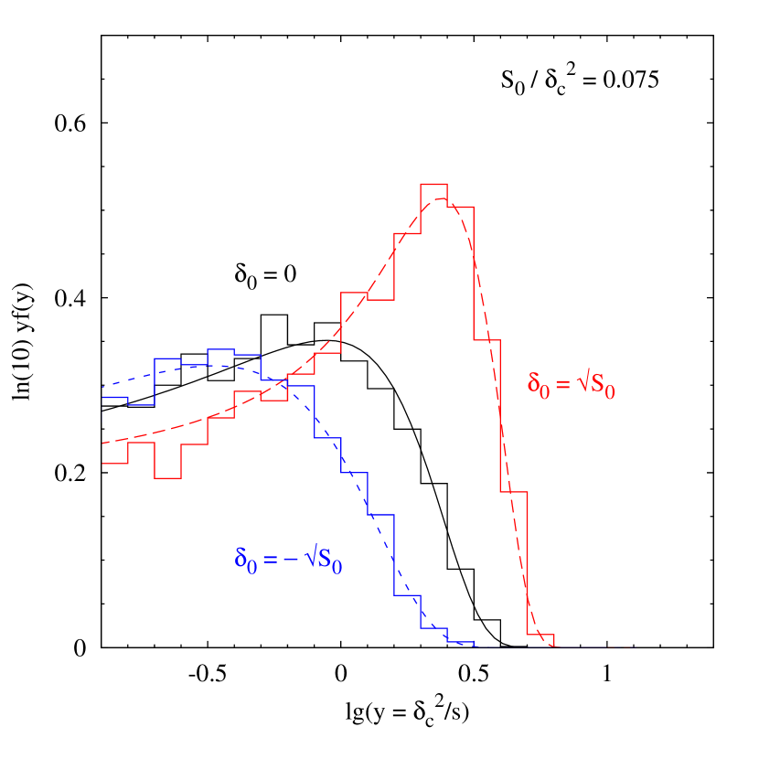
Figure 2 compares the prediction in equation (28) with a Monte Carlo solution of the conditional first crossing distribution. The comparison is for Gaussian filtered random walks using a power spectrum $P(k)\propto k^{-1.2}$. The numerical treatment uses the algorithm of Bond et al. (1991) and was described in Paranjape et al. (2012). The histograms are the same as in Figure 6 of Paranjape et al. and show the distribution of first crossing scales for a constant barrier, for walks that were required to pass through the indicated values of $\delta_{0}$ at scale $S_{0}$, for two choices of $S_{0}$. We see that the analytic prediction works very well in describing the numerical solution.

Figure 3: Same as lower panel of Figure 2, but for a larger value of $|\delta_{0}|$, and note that now the $y$-axis is on a log scale. The analytic prediction equation (28) for $\delta_{0}=0.9\delta_{\rm c}$ describes the sharp peak in the numerical solution remarkably accurately. It begins overestimating the numerical solution around ${\rm log}_{10}\nu^{2}\simeq 0.4$, at which point about 75% of the probability has been accounted for (see text for why this happens).

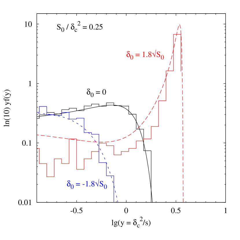
This good agreement is despite the fact that equation (26) formally ignores walks which might have crossed the barrier prior to $S_{0}$. This can be understood by the fact that the values of $\delta_{0}$ being considered in Figure 2 are significantly smaller than $\delta_{\rm c}$, so that very few of the walks would have reached the barrier prior to $S_{0}$ and then returned to pass through $\delta_{0}$ at $S_{0}$. One can then ask whether the expression in equation (28) would continue to be accurate even for $\delta_{0}\lesssim\delta_{\rm c}$, since this is the regime of interest for calculations of merger rates.

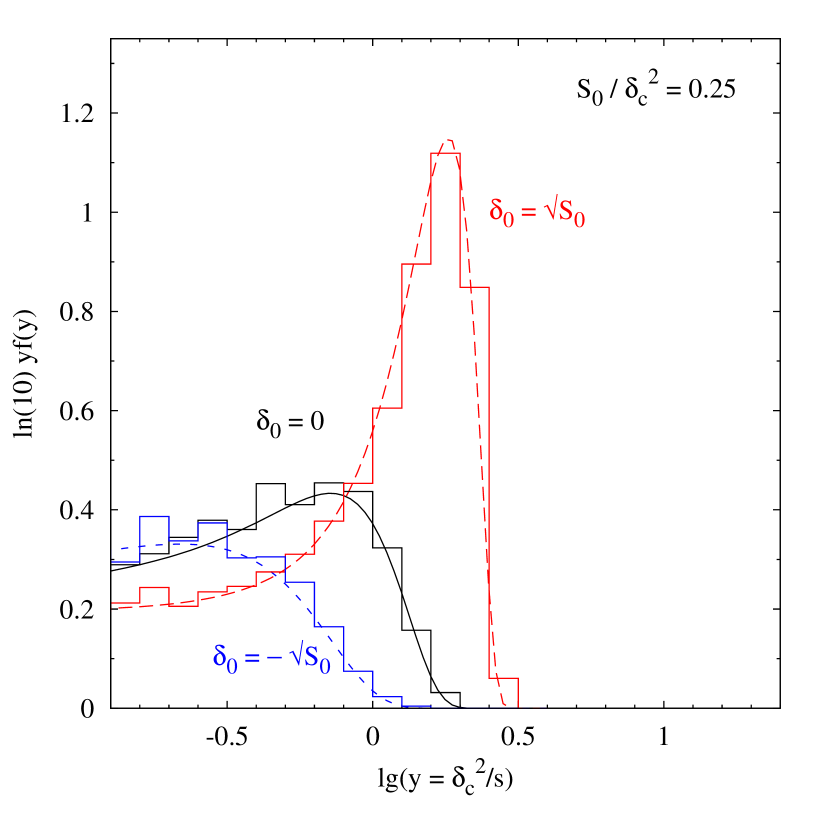
We test this in Figure 3, which compares equation (28) with the Monte Carlo solution for the same choice of conditioning scale $S_{0}$ as in the lower panel of Figure 2, but with a larger magnitude for $\delta_{0}$ which is now $|\delta_{0}|=0.9\delta_{\rm c}$. We see that for $\delta_{0}=+0.9\delta_{\rm c}$, the numerical solution has a sharp peak which is very well described by equation (28). The latter starts overestimating the numerical answer around ${\rm log}_{10}\nu^{2}\simeq 0.4$, which can be understood as follows.

Paranjape et al. (2012) demonstrated in their Figure 7 that the numerical conditional distributions are, to a good approximation, related to the corresponding unconditional one by a simple scaling relation which sends $\nu\to\nu_{10}=\delta_{{\rm c}\times}/\sqrt{sQ}$ in the unconditional distribution. This is also approximately true of the analytic expression in equation (28). Since equation (24) is not a good approximation to the unconditional first crossing distribution at small values of $\nu$ (Musso & Sheth 2012), it follows that the corresponding analytic conditional distribution will not be a good approximation at small $\nu_{10}$. One can check that, for the choices of $S_{0}$ and $\delta_{0}$ in Figure 3, $\nu_{10}$ actually passes through zero and becomes negative around ${\rm log}_{10}\nu^{2}\simeq 0.5$. So the mismatch between the analytic prediction and the numerical solution is not surprising. In practice, $\int_{0.4\ln 10}^{-\ln S_{0}}d\ln y\,yf(y|S_{0})=0.75$, indicating that the prediction is inaccurate only for the 25% which cross at the largest values of $s$ (smallest values of $y$).

3.5 Halo bias with correlated steps

Now that we have in hand a good approximation to the conditional first crossing distribution, we can turn to the associated description of halo bias.

Figure 4: Distribution of the height $\delta_{0}$ on scale $S_{0}$  of walks which have not crossed $\delta_{\rm c}$ prior to $S_{0}$, for a range of choices of $S_{0}$ (histograms), measured in the same Monte-Carlo simulations which were used to make the Figures 2 and 3. Dashed curves show that a Gaussian, truncated at $\delta_{0}=\delta_{\rm c}$, provides a good approximation. Note that $S_{0}/\delta_{c}^{2}=300\times 0.05^{2}=3/4$ corresponds to smoothing scales which are of order that associated with a typical halo: therefore, if one restricts attention to smaller $S_{0}$, then ignoring the truncation of the Gaussian should be a good approximation.

The first issue that we would like to address is if Hermite polynomials of the smoothed matter density field are still special. Appendix B suggests that they are, as long as the underlying matter density field is Gaussian. More formally, we show there that the rôle of the Hermite polynomial $H_{n}(\delta_{0}/\sqrt{S_{0}})$ in the average is that of removing from it all the disconnected parts, so that only the connected part of the expectation value of $\delta_{0}^{n}$ remains.

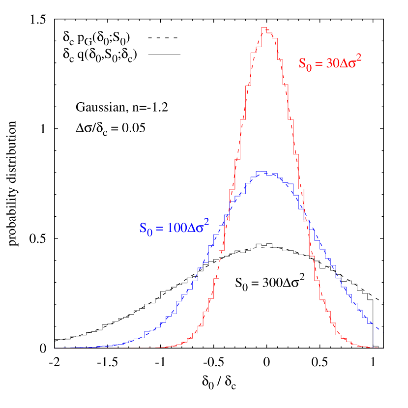
Secondly, for reasons discussed in section 2.3, in principle we must specify the probability distribution $q(\delta_{0},S_{0};\delta_{\rm c})$ to be used in the average. In the present case, $q$ is not known analytically. However, in the spirit of Musso & Sheth (2012), we can argue that the error in ignoring the difference between $p$ and $q$ is of the same order as that already included in $f(s|\delta_{0},S_{0})$. Indeed, the fact that the conditional distributions shown in Figure 2 are such an accurate description of the numerical solution means that, in this case, the approximation is consistent. This is a consequence of the fact that for correlated steps zig-zags are exponentially rare at small $S_{0}$; in this limit, $p\approx q$. We can test this explicitly by looking directly at the distribution of $q$ in our Monte-Carlos. Figure 4 shows that, for $S_{0}$ values which are smaller than those associated with typical halos, the difference between $q$ and the Gaussian is almost negligible.

Motivated by this simplification, let us define the real-space bias coefficients associated with the conditional distribution $f(s|\delta_{0},S_{0})$ using

$$b_{n} \equiv\frac{1}{S_{0}^{n/2}}\left\langle\,(1+\delta_{\rm h})H_{n}(\delta_{0}/\sqrt{S_{0}})\,\right\rangle$$

$$=\int_{-\infty}^{\infty}{\rm d}\delta_{0}\,p_{\rm G}(\delta_{0};S_{0})\left\langle\,1+\delta_{\rm h}|\delta_{0},S_{0}\,\right\rangle H_{n}(\delta_{0}/\sqrt{S_{0}})\,,$$ (32)

with $\left\langle\,1+\delta_{\rm h}|\delta_{0},S_{0}\,\right\rangle$ given in equation (2). Below we will show comparisons between numerical measurements of these quantities ($q$-averaged by construction) with analytic results using the $p$-averaged expression in the second line of (32). From the discussion above, we expect these to match well at least for the smallest $S_{0}$ shown in Figure 4.

For $f(s|\delta_{0},S_{0})$ given by equation (26), some algebra brings these into the form (see Appendix A.2)

$$b_{n}=\frac{(-S_{\times}/S_{0})^{n}}{f(s)}\int_{0}^{\infty}{\rm d}\delta^{\prime}\delta^{\prime}\left(\frac{\partial}{\partial\delta_{\rm c}}+\frac{\epsilon_{\times}}{2s}\frac{\partial}{\partial\delta^{\prime}}\right)^{\!n}\!p(\delta_{\rm c},\delta^{\prime})\,,$$ (33)

with $f(s)$ given in equation (21). Appendix A.3 shows that

$$f(s|\delta_{0},S_{0}) =\sum_{n=0}^{\infty}\frac{\delta_{0}^{n}}{n!}\left(-\frac{S_{\times}}{S_{0}}\right)^{n}\int_{0}^{\infty}{\rm d}\delta^{\prime}\delta^{\prime}$$

$$\phantom{\sum}\times\left(\frac{\partial}{\partial\delta_{\rm c}}+\frac{\epsilon_{\times}}{2s}\frac{\partial}{\partial\delta^{\prime}}\right)^{\!n}\!p_{\rm G}(\Delta;\mathbf{C}-\tilde{}\mathbf{c})\,,$$ (34)

holds exactly for the distribution (26), where $\Delta=(\delta_{\rm c},\delta^{\prime})$ and the matrices $\mathbf{C}$ and $\tilde{}\mathbf{c}$ were defined in equation (14). Since the bivariate Gaussian $p_{\rm G}(\Delta;\mathbf{C})$ is precisely the distribution $p(\delta_{\rm c},\delta^{\prime})$ that appears in equation (33), we clearly have

$$\frac{f(s|\delta_{0},\tilde{}\mathbf{c}=0)}{f(s)}=1+\sum_{n=1}^{\infty}\frac{\delta_{0}^{n}}{n!}b_{n}\,.$$ (35)

Setting $\tilde{}\mathbf{c}=0$ corresponds to the following assignments in equation (28):

$$Q\to 1~{}~{};\qquad\bar{\sigma}\sqrt{s}\to(2\Gamma)^{-1}\,;$$

$${\bar{\delta}^{\prime}}/\bar{\sigma}\to\Gamma\nu\left[1-(\delta_{0}/\delta_{\rm c})(S_{\times}/S_{0})(1-\epsilon_{\times})\right].$$ (36)

As a result (see Appendix A.4) the bias coefficients can be reduced to:

$$\delta_{\rm c}^{n}b_{n}=\left(\frac{S_{\times}}{S_{0}}\right)^{n}(\alpha_{n}+\beta_{n}+\gamma_{n})\,,$$ (37)

where

$$\alpha_{n} =\nu^{n}H_{n}(\nu)\,,~{}~{}n\geq 1\,,$$ (38)

$$\beta_{n} =\frac{1}{1+A}\begin{cases}-A\left(1-\epsilon_{\times}\right)&,\,n=1\\ \left(1-\epsilon_{\times}\right)^{n}(\Gamma\nu)^{n}H_{n-2}(\Gamma\nu)&,\,n\geq 2\end{cases}$$ (39)

$$\gamma_{n} =\begin{cases}0&,~{}~{}n=1\\ \sum_{k=1}^{n-1}\binom{n}{k}\alpha_{k}\beta_{n-k}&,~{}~{}n\geq 2\,,\end{cases}$$ (40)

where $A$ was defined in equation (25).

Figure 5: Comparison of bias coefficients $b_{1}$ and $b_{2}$ of equation (37) (smooth curves) with corresponding measurements (points with Poisson errors) in the same Monte Carlo simulations used in Figures 2 and 3, for a range of $S_{0}$ values. The measurements were performed as described in section 2.3. The analytic prediction clearly tracks both the $s$- and $S_{0}$-dependence fairly accurately. There are small systematic differences, especially at large $s$, which arise because $q\neq p$ at large $S_{0}$, and our analytic approximation to $f(s|\delta_{0},S_{0})$ stops being a good approximation when $s\gg S_{0}$.

There are some interesting parallels with the calculation for sharp-$k$ walks, and some important differences. There is obviously a close analogy between the $S_{0}\to 0$ limit of sharp-$k$ walks and the $\tilde{}\mathbf{c}\to 0$ limit for correlated steps, especially since the matrix $\tilde{}\mathbf{c}$ is proportional to $S_{0}$ (c.f. equation 14, noting that the factor $S_{\times}/S_{0}$ becomes constant as $S_{0}\to 0$). However, in the present case one is not throwing away all the dependence on $S_{0}$, since factors of $\epsilon_{\times}$ explicitly appear in the expression for the $b_{n}$. In particular, these factors of $\epsilon_{\times}$ would not have appeared if we had simply taken derivatives of the unconditional distribution (equation 24) with respect to $\delta_{\rm c}$. This has an important consequence: for sharp-$k$ filtering, the quantities $b_{n}$ were independent of $S_{0}$, whereas here they depend explicitly on $S_{0}$. If we write equation (37) as

$$b_{n}\sim(S_{\times}/S_{0})^{n}\sum_{k=0}^{n}b_{nk}\,\epsilon_{\times}^{k},$$ (41)

then it is the quantities $b_{nk}$ (rather than $b_{n}$) which are scale-independent. This will be important below when interpreting our results in terms of Fourier-space bias. Note that the $b_{n0}$ are the peak-background split parameters $f^{-1}(-\partial/\partial\delta_{\rm c})^{n}f$ which are of most interest in cosmological applications. This is obvious upon setting $\epsilon_{\times}\to 0$ in equation (33).

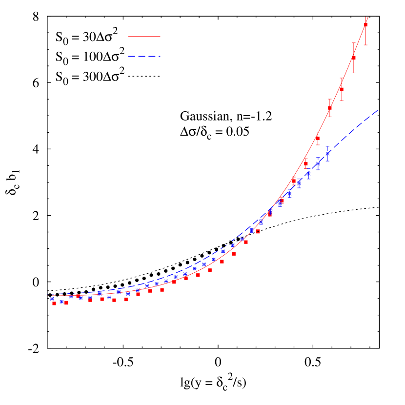
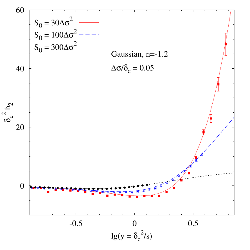
Since $p\approx q$, in contrast to when steps are uncorrelated, one might expect equation (33) to be quite accurate. We test this explicitly in Figure 5 by comparing the results of evaluating the r.h.s. of equation (33) for $n=1$ and $n=2$ with corresponding measurements (performed as described in section 2.3) using the same Monte Carlo simulations that were used in Figures 2 and 3. By construction, the numerically estimated quantity is $q$-averaged, whereas the analytic curves show the Gaussian-averaged coefficients in equation (32). The analytic predictions closely track the measurements over a range of $s$-values for several choices of $S_{0}$. There are small systematic deviations which are likely due to a combination of the facts that $q\neq p$ at large $S_{0}$ and that the analytic prediction fails to be a good approximation at large $s$.

Since ignoring the difference between $p$ and $q$ is a good approximation, one might wonder if the effect of $\epsilon_{\times}$ can also be ignored; naively one expects the $q$-averaging to be irrelevant at small $S_{0}/s$ where $\epsilon_{\times}$ is also likely to be small. Figure 6 shows the results for $b_{1}$ and $b_{2}$ for one of the choices of $S_{0}$ from Figure 5, comparing the same measurements as in that figure with analytic expressions in which $\epsilon_{\times}$ is retained as per equations (39) and (40) (solid curves) or set to zero by hand (dashed curves). We see that the terms involving $\epsilon_{\times}$ contribute significantly and must be retained to get an accurate description of the bias.

3.6 Recovery of scale-independent bias factors

The bias coefficients in Figure 5 show a strong dependence on the scale $S_{0}$. This is rather different from the case of sharp-$k$ filtering, for which the $b_{n}$ recovered from $p$-averaging (equation 7) were independent of $S_{0}$. Indeed, the scale-independence of the recovered $b_{n}$ was one of our motivations for cross-correlating with the Hermite-transformed field in the first place, so it is interesting to ask if the dependence on $S_{0}$ can be removed.

Figure 6: Same as Figure 5 for one choice of $S_{0}$, but comparing the numerical answer for $b_{1}$ and $b_{2}$ with the analytic prediction equation (37) when the dependence on $\epsilon_{\times}$ is retained (solid red) or set to zero by hand (dashed blue). Clearly, retaining the dependence on $\epsilon_{\times}$ is important, indicating that our method is sensitive to the $k$-dependence of bias (see text). Black triangles show the result of implementing the recursive procedure described in the text for reconstructing the usual ($k$-independent) peak-background split parameters $b_{10}$ and $b_{20}$ (dotted curves) from these measurements. Although defined at finite $S_{0}$, the procedure works well in reproducing the $S_{0}$-independent $b_{n0}$.

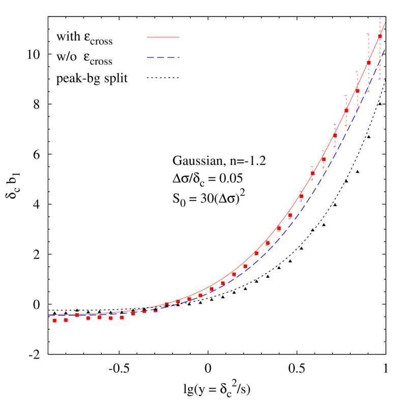
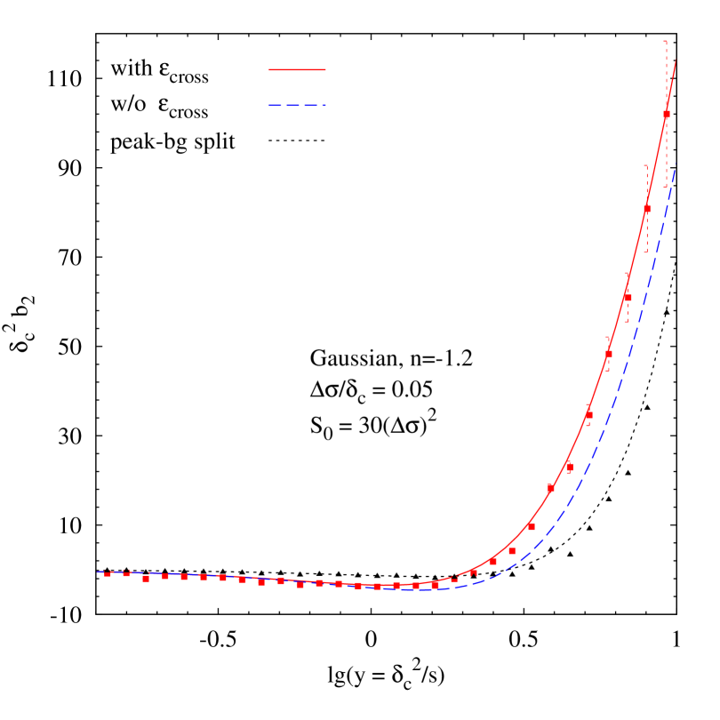
This turns out to be possible because of the following. First, the scale dependence of $b_{n}$ is almost entirely due to the factors of $S_{\times}$ and $\epsilon_{\times}$ (the other effect comes from the small difference between $p$ and $q$ averaging). And secondly, equation (37) shows that the scale-independent $b_{nk}$ are linearly related to each other in such a way that measuring $b_{1},\ldots,b_{n}$ is sufficient to recover all the $b_{1k},\ldots b_{nk}$.

We demonstrate this explicitly for $n=1$ and $2$. For $n=1$, we can write

$$b_{1} =\frac{1}{\delta_{\rm c}}\frac{S_{\times}}{S_{0}}\left[\left(\nu^{2}-\frac{A}{1+A}\right)+\epsilon_{\times}\frac{A}{1+A}\right]$$

$$\equiv\frac{S_{\times}}{S_{0}}(b_{10}+\epsilon_{\times}b_{11})\,.$$ (42)

Since

$$\delta_{\rm c}\,b_{11}=\nu^{2}-\delta_{\rm c}b_{10}\,,$$ (43)

we can estimate

$$\delta_{\rm c}\,b_{10}=\frac{\delta_{\rm c}\,(S_{0}/S_{\times})b_{1}-\epsilon_{\times}\nu^{2}}{1-\epsilon_{\times}}.$$ (44)

Similarly,

$$b_{2}=\left(\frac{S_{\times}}{S_{0}}\right)^{2}\left(b_{20}+2\epsilon_{\times}\,b_{21}+\epsilon_{\times}^{2}b_{22}\right)\,,$$ (45)

where the excursion set predictions for the coefficients $b_{2j}$ can be read off from equation (37). For example, $\delta_{\rm c}^{2}\,b_{21}=\nu^{2}(A-\Gamma^{2})/(1+A)$. But, more relevant to the present discussion, we find

$$\delta_{\rm c}^{2}b_{21} =\nu^{2}(\delta_{\rm c}b_{10}-1)-\delta_{\rm c}^{2}b_{20}$$

$$\delta_{\rm c}^{2}b_{22} =\delta_{\rm c}^{2}b_{20}+\nu^{2}(\nu^{2}-2\delta_{\rm c}b_{10}+1)\,.$$ (46)

Hence,

$$\delta_{\rm c}^{2}\,b_{20}= \frac{1}{\left(1-\epsilon_{\times}\right)^{2}}\bigg{[}\delta_{\rm c}^{2}\bigg{(}\frac{S_{0}}{S_{\times}}\bigg{)}^{\!2}b_{2}$$

$$-\epsilon_{\times}\nu^{2}\,\bigg{(}2\delta_{\rm c}\frac{S_{0}}{S_{\times}}b_{1}-\epsilon_{\times}(\nu^{2}-1)-2\bigg{)}\bigg{]}\,.$$ (47)

We have deliberately isolated the peak-background split parameters $b_{n0}$ above. From the structure of the coefficients in equation (37) it is clear that this reconstruction can be extended to the higher order coefficients as well.

The dotted curves in Figure 6 show the analytic predictions for $b_{10}$ and $b_{20}$ from equation (37), while the triangular symbols show the numerical estimates using equations (44), (47) and the corresponding measurements of $b_{1}$ and $b_{2}$. Clearly, the reconstruction works well. Moreover, since we are working at finite $S_{0}$, our procedure has allowed a simple and direct estimate of the peak-background split parameters $b_{n0}$ from a measurement of scale-dependent bias, without having to access very large scales. E.g., the Figure shows results for $S_{0}=0.075\,\delta_{\rm c}^{2}$, which corresponds to the scale associated with a $\nu\approx 3.7$ halo and a Lagrangian length scale of $R_{0}\sim 17h^{-1}$Mpc; most other analyses of halo bias are restricted to length scales which are several times larger.

Another way to see this is to notice that, in the expressions above, $b_{n}\to b_{n0}$ when $\epsilon_{\times}\to 0$. Since $\epsilon_{\times}\to 0$ on large scales, the analysis above shows explicitly that our method for reconstructing $b_{n0}$ works even on the smaller scales where $\epsilon_{\times}\neq 0$. Indeed, although we have concentrated on isolating $b_{n0}$, the analysis above shows that we can isolate the other $b_{nk}$ as well. For example, having measured $b_{1}$ and $b_{2}$ using our Hermite-weighting scheme, and having used equations (44) and (47) to estimate $b_{10}$ and $b_{20}$, equation (46) furnishes estimates of $b_{21}$ and $b_{22}$.

The expressions above show that our method will break if $\epsilon_{\times}=1$, which happens when $s\to S_{0}$. This is not surprising since this is the limit in which the large scale environment is the same as that on which the halo was defined, so our expressions for the conditional distribution are becoming ill-defined. Since this regime is substantially smaller than the one of most interest in cosmology, we conclude that our method allows a substantial range of interesting scales to provide estimates of the bias factors $b_{nk}$.

3.7 Real and Fourier-space bias

The appearance of $\epsilon_{\times}$ in the real-space expressions for $b_{n}$ generically indicates that the bias in Fourier space must be $k$-dependent. This is most easily seen with $b_{1}$ using a Gaussian filter $W(kR)={\rm e}^{-k^{2}R^{2}/2}$.

Suppose that

$$\delta_{0}(\mathbf{k})=\delta(\mathbf{k})W(kR_{0})$$ (48)

and

$$\delta_{\rm h}(\mathbf{k})=b_{1}(\mathbf{k})\delta(\mathbf{k})W(kR)\,,$$ (49)

so that in real space $\left\langle\,\delta_{\rm h}|\delta_{0}\,\right\rangle=\delta_{0}\left\langle\,\delta_{\rm h}\delta_{0}\,\right\rangle/S_{0}$. Then equation (42) implies that

$$b_{1}(\mathbf{k})=b_{10}+\frac{k^{2}s}{\sigma_{1}^{2}}b_{11}\,.$$ (50)

This shows that the excursion set analysis makes a prediction for how the Fourier-space coefficients $b_{10}$ and $b_{11}$ should depend on $\nu=\delta_{c}/\sigma$ and $\Gamma$.

It is remarkable that peaks theory predicts this same structure (constant plus $k^{2}$) for the linear Fourier space bias factor (Desjacques et al. 2010). Although the coefficients $b_{10}$ and $b_{11}$ for peaks differ from that for the excursion set halos studied here, the relation (43) between these coefficients is the same. We have checked explicitly that peaks also satisfy the relationships between the second order bias coefficients as shown in equation (47) (although the actual values of $b_{20}$, $b_{21}$ and $b_{22}$ are different), and so we expect this correspondence between the $k$-dependence of peak and halo-bias will hold for all $n$. Because this correspondence is seen in two very different analyses (excursion sets and peaks), there is likely to be a deeper reason for its existence.

We explore this further in Appendix B where we discuss the relation between our analysis and the work of Matsubara (2011) who has argued that $k$-dependent bias factors are generically associated with nonlocal biasing schemes. He provides a number of generic results for such nonlocal bias, noting that the Fourier-space structure at order $n$ which can be written in terms of what he calls renormalized bias coefficients $c_{n}(\mathbf{k}_{1},\ldots,\mathbf{k}_{n})$. For peaks theory,

$$c_{n}(\mathbf{k}_{1},\ldots,\mathbf{k}_{n}) =b_{n0}+b_{n1}\sum_{i}k_{i}^{2}+b_{n2}\sum_{i<j}k_{i}^{2}k_{j}^{2}+\ldots.$$ (51)

In this case, for Gaussian initial conditions, the Hermite-weighted averages (with a Gaussian filter as per equation 62) show a structure that is identical to our excursion set predictions of (41). More generally, our Hermite-weighting scheme provides a practical way of measuring integrals of Matsubara’s renormalized bias coefficients $c_{n}$.

We therefore conclude that our real-space Hermite-weighted prescription for measuring halo bias can allow us to separate the scale-dependent contribution to bias as well as isolate the scale-independent (peak-background split) part arising from each order $n$, which traditional Fourier-space measurements cannot do. The specific results of our excursion set analysis (e.g., the relations between the $b_{nk}$) are then predictions that can be tested in more realistic settings such as $N$-body simulations. But this is beyond the scope of the present work.

4 Conclusions and discussion

We provided an analytic approximation for the first crossing distribution for walks with correlated steps which are constrained to pass through a specified position (equation 28), and showed that it was accurate (Figure 2). Although this is interesting in its own right, we did not explore this further. Rather, we used it to provide a simple analytic expression for the large scale halo bias factors (equation 37), showing that, as a result of correlations between scales, real space measures of halo bias are scale dependent (equation 41 and Figure 5), but this scale dependence is best thought of as arising from $k$-dependent bias in Fourier space (Section 3.7). Although we presented comparisons with numerical results for a specific choice of filter (Gaussian) and power spectrum ($P(k)\propto k^{-1.2}$), the results of Musso & Sheth (2012) lead us to expect that our analytical results will be equally accurate for other filters and power spectra, including TopHat filtered $\Lambda$CDM.

For correlations which arise because of a Gaussian smoothing filter, the linear bias factor $b_{1}$ is a constant plus a term which is proportional to $k^{2}$. This is a consequence of the fact that our analysis is based on the approximation of Musso & Sheth (2012), which associates halos with places where the height of the smoothed field and its first derivative with respect to smoothing scale satisfy certain constraints. If constraining the second derivative as well leads to an even more accurate model of the first crossing distribution, then this would give rise to $k^{4}$-dependence in the bias. It is in this sense that $k$-dependent halo bias is part and parcel of the excursion set approach. Such $k$-dependence will lead to stochasticity in real space measures of bias (Desjacques & Sheth 2010); we have not pursued this further.

We also provided an algorithm for estimating the scale-independent coefficients of the $k$-dependent bias factors from real space measurements (Section 3.6). Although the method uses cross-correlations between the halo field and suitably transformed versions of the smoothed mass field at the same spatial position (equation 32), the bias factors it returns are independent of the scale on which this transformation is done (Figure 6). In particular, the coefficient of the $k$-independent part of the bias which our algorithm returns equals that associated with the peak-background split argument, even though our algorithm can be applied on scales for which the usual formulation of the peak-background split argument does not apply.

For Gaussian fields, the transformation we advocate uses the Hermite polynomials. Therefore, our work has an interesting connection to Szalay (1988) who noted that, instead of defining bias coefficients by writing $\delta_{\rm h}$ as a Taylor series in $\delta_{0}$ as is usually done, one could have chosen to expand the mass field in Hermite polynomials. Our analysis shows that this is indeed a fruitful way to proceed, even when the bias factors are $k$-dependent.

There are two reasons why this is remarkable. First, our analysis shows that, for the excursion set model, the coefficients of the expansion in $\delta_{0}$ are the same as those for the expansion in Hermite polynomials (equations 32 and 35). There is no reason why this should be true in general. And second, Szalay explicitly assumed that halo bias was ‘local’: $\delta_{\rm h}$ was a function of $\delta_{0}$ only. For local bias, the bias factors are $k$-independent; $k$-dependent bias factors are a signature that the bias is nonlocal (Matsubara 2011, with the $k$-dependence of peak bias discussed in Desjacques et al. 2010 being a specific example), so it is not a priori obvious that an expansion in Hermite polynomials would have been useful.

In Appendix B we showed why, even for nonlocally biased tracers of a Gaussian field, the Hermites are so special. For completeness, we also provided an analysis of the general case, in which the underlying field is not necessarily Gaussian (equation 78). This more general analysis may prove useful should it turn out that the primordial fluctuation field was non-Gaussian, or if one wishes to describe halo bias with respect to the nonlinear Eulerian field rather than with respect to the initial one.

In the former case, primordial non-Gaussianity is expected to be sufficiently weak that the Edgeworth expansion can be used to provide insight into the expected modifications to halo abundances. Since Hermites play an important role in the Edgeworth expansion, it is likely that our Hermite-based algorithm for halo bias will be useful for constraining $f_{\rm NL}$.

Recent work has emphasized the advantages of using cross- rather than auto-correlations to estimate halo bias (Smith et al. 2007; Pollack et al. 2012). Since $H_{n}$ is an $n$-th order polynomial in the mass field, one may think of our algorithm as an extension of this program: it uses two-scale halo-mass cross-correlations at the same real-space position to extract information which is usually obtained from $n$-point statistics. However, in addition to being simpler, our algorithm is able to estimate the bias coefficients on smaller scales than those on which the more traditional analyses $n$-point (Fourier or real-space) analyses are performed. So we expect it to find use in analyses of halo bias in simulations, and galaxy bias in real datasets.

For example, one can compare our prescription with traditional methods of estimating bias in real space, e.g. Manera & Gaztañaga (2012). Here, instead of computing averages of the matter field centered at locations of halos (as is natural in the excursion set approach), one explicitly defines a halo field $\delta_{\rm h}(\mathbf{x})$ smoothed on a grid of cell-size $R_{0}$ and uses the matter field $\delta_{0}(\mathbf{x})$ smoothed on the same grid. One then fits a polynomial of the type $\delta_{\rm h}=b_{0}+b_{1}\delta_{0}+b_{2}\delta_{0}^{2}/2$ to a scatter plot of $\delta_{\rm h}$ vs. $\delta_{0}$ using a least squares prescription. This is conceptually the same as approximating the function $\left\langle\,\delta_{\rm h}|\delta_{0}\,\right\rangle$ (which is most easily seen by considering linear biasing of a Gaussian field, for which the statement is exact). This can be compared with the excursion set prediction $\left\langle\,1+\delta_{\rm h}|\delta_{0}\,\right\rangle=f(s|\delta_{0},S_{0})/f(s)$, and we see that the coefficients obtained from the fit will generically depend on $S_{0}$. As Manera & Gaztañaga show, one needs to define a grid on very large scales ($R_{0}\gtrsim 40h^{-1}$Mpc) in order to recover scale independent bias coefficients. On the other hand, our prescription can in principle operate at much smaller scales (c.f. section 3.6) and remove this scale dependence by basically computing weighted integrals of the mean relation in the $\delta_{\rm h}$-$\delta_{0}$ scatter plot. A more detailed comparison with traditional techniques is complicated by the fact that we have made predictions for Lagrangian bias whereas analyses such as Manera & Gaztañaga’s typically work in the final, Eulerian field. We leave such a comparison to future work.

In this context, it is worth noting that our algorithm is more than just a simple way of estimating the nonlinear bias coefficients $b_{n}$. For example, there has been recent interest in reducing the stochasticity between the underlying mass field and that defined by the biased tracers (Hamaus et al. 2010; Cai et al. 2011). Some of this stochasticity is due to the nonlinear nature of the bias (Hamaus et al. 2011). Our demonstration that the nonlinear bias factors measure the amplitude of the cross-correlation function between the halo field and the Hermite-transformed mass field will simplify such analyses.

Appendix A Details of calculations

In this Appendix we sketch the proofs of various identities stated in the main text.

A.1 Proof of equation (7)

To prove equation (7) for sharp-$k$ walks, it is useful to consider the following Fourier transform relations involving the Hermite polynomials, which follow from the definition of the $H_{n}$:

$$\frac{{\rm e}^{-x^{2}/2}}{\sqrt{2\pi}}H_{n}(x) =\int_{-\infty}^{\infty}\frac{{\rm d}k}{(2\pi)}{\rm e}^{ikx}(-ik)^{n}{\rm e}^{-k^{2}/2}$$

$$(-ik)^{n}{\rm e}^{-k^{2}/2} =\int_{-\infty}^{\infty}\frac{{\rm d}x}{\sqrt{2\pi}}{\rm e}^{-ikx}{\rm e}^{-x^{2}/2}H_{n}(x)\,.$$ (52)

For the conditional first crossing distribution of equation (3), we use the relation

$$sf_{\rm u}(s|\delta_{0},S_{0}) =s\left(-\frac{\partial}{\partial\delta_{\rm c}}\right)p_{\rm G}(\delta_{0}-\delta_{\rm c};s-S_{0})\,.$$ (53)

Using $y_{0}\equiv\delta_{0}/\sqrt{S_{0}}$ and $\nu=\delta_{\rm c}/\sqrt{s}$ one can write

$$\left\langle\,sf_{\rm u}(s|\delta_{0},S_{0})H_{n}(\delta_{0}/\sqrt{S_{0}})\,\right\rangle$$

$$\phantom{sf(s)}=-\frac{\partial}{\partial\nu}\int_{-\infty}^{\infty}\frac{{\rm d}y_{0}}{2\pi}\frac{{\rm e}^{-y_{0}^{2}/2}H_{n}(y_{0})}{\sqrt{1-S_{0}/s}}{\rm e}^{-\frac{(y_{0}-\nu\sqrt{s/S_{0}})^{2}}{2(s/S_{0}-1)}}$$

$$\phantom{sf(s)}=-\left(\frac{S_{0}}{s}\right)^{n/2}\frac{\partial}{\partial\nu}\int_{-\infty}^{\infty}\frac{{\rm d}k}{2\pi}(-ik)^{n}{\rm e}^{ik\nu-k^{2}/2}$$

$$\phantom{sf(s)}=\left(\frac{S_{0}}{s}\right)^{n/2}\frac{1}{\sqrt{2\pi}}{\rm e}^{-\nu^{2}/2}H_{n+1}(\nu)\,,$$ (54)

where the second equality follows from writing the Fourier integrals corresponding to the Hermite polynomial and the Gaussian in $(y_{0}-\nu\sqrt{s/S_{0}})$, doing the integral over $y_{0}$ to give a Dirac delta and using this to perform one Fourier-space integral. The third equality then follows from equation (52). Together with $sf_{\rm u}(s)=(2\pi)^{-1/2}\nu\,{\rm e}^{-\nu^{2}/2}$, this gives the result.

A.2 Form of bias coefficients in equation (33)

The weighted average of the distribution (26) is

$$\left\langle\,f(s|\delta_{0},S_{0})H_{n}(\delta_{0}/\sqrt{S_{0}})\,\right\rangle$$

$$=\int_{0}^{\infty}\!\!{\rm d}\delta^{\prime}\delta^{\prime}\!\int{\rm d}\delta_{0}\,p_{\rm G}(\delta_{0};S_{0})H_{n}\!\!\left(\frac{\delta_{0}}{\sqrt{S_{0}}}\right)p(\delta_{\rm c},\delta^{\prime}|\delta_{0})\,.$$ (55)

The product $p_{\rm G}(\delta_{0};S_{0})H_{n}(\delta_{0}/\sqrt{S_{0}})$ and the bivariate Gaussian $p(\delta_{\rm c},\delta^{\prime}|\delta_{0})$ (equation 27) can be expressed in terms of their Fourier transforms: i.e., we use equation (52) and

$$p(\delta_{\rm c},\delta^{\prime}|\delta_{0}) =\int\frac{{\rm d}^{2}k}{(2\pi)^{2}}{\rm e}^{i\mathbf{k}^{\rm T}(\Delta-\bar{}\mathbf{x})}{\rm e}^{-\frac{1}{2}\mathbf{k}^{\rm T}(\mathbf{C}-\tilde{}\mathbf{c})\mathbf{k}}\,,$$ (56)

with $\Delta=(\delta_{\rm c},\delta^{\prime})$ and $\bar{}\mathbf{x}$, $\mathbf{C}$ and $\tilde{}\mathbf{c}$ given by equation (15) and (14), respectively. The integral over $\delta_{0}$ then gives a one-dimensional Dirac delta $\delta_{\rm D}\left(k_{0}-kS_{\times}/S_{0}-k^{\prime}\epsilon_{\times}S_{\times}/2sS_{0}\right)$ where $k_{0}$, $k$ and $k^{\prime}$ are the Fourier variables corresponding to $\delta_{0}$, $\delta_{\rm c}$ and $\delta^{\prime}$, respectively. Performing the $k_{0}$ integral gives an expression in which the contribution of the “correction” matrix $\tilde{}\mathbf{c}$ exactly cancels. The result can be expressed as

$$\frac{1}{S_{0}^{n/2}}\left\langle\,f(s|\delta_{0},S_{0})H_{n}(\delta_{0}/\sqrt{S_{0}})\,\right\rangle$$

$$=\left(-\frac{S_{\times}}{S_{0}}\right)^{\!n}\!\int_{0}^{\infty}\!{\rm d}\delta^{\prime}\delta^{\prime}\left(\frac{\partial}{\partial\delta_{\rm c}}+\frac{\epsilon_{\times}}{2s}\frac{\partial}{\partial\delta^{\prime}}\right)^{\!n}p(\delta_{\rm c},\delta^{\prime})\,,$$ (57)

and using $\left\langle\,1+\delta_{\rm h}|\delta_{0},S_{0}\,\right\rangle\equiv f(s|\delta_{0},S_{0})/f(s)$ gives the result (33).

A.3 Taylor expansion of the conditional first crossing distribution in equation (34)

Using equation (27) and the shorthand notation $p_{\rm G}$ for $p_{\rm G}(\Delta;\mathbf{C}-\tilde{}\mathbf{c})$ where $\Delta=(\delta_{\rm c},\delta^{\prime})$ and the matrices $\mathbf{C}$ and $\tilde{}\mathbf{c}$ were defined in equation (14), straightforward algebra shows that

$$p(\delta_{\rm c},\delta^{\prime}|\delta_{0})$$

$$=\sum_{m,n=0}^{\infty}\frac{(-\delta_{0}S_{\times}/S_{0})^{m+n}}{m!n!}\left(\frac{\partial}{\partial\delta_{\rm c}}\right)^{m}\!\left(\frac{\epsilon_{\times}}{2s}\frac{\partial}{\partial\delta^{\prime}}\right)^{\!n}p_{\rm G}$$

$$=\sum_{k=0}^{\infty}\frac{\delta_{0}^{k}}{k!}\left(-\frac{S_{\times}}{S_{0}}\right)^{\!k}\sum_{n=0}^{k}\binom{k}{n}\left(\frac{\partial}{\partial\delta_{\rm c}}\right)^{\!n}\!\left(\frac{\epsilon_{\times}}{2s}\frac{\partial}{\partial\delta^{\prime}}\right)^{\!k-n}p_{\rm G}$$

$$=\sum_{k=0}^{\infty}\frac{\delta_{0}^{k}}{k!}\left(-\frac{S_{\times}}{S_{0}}\right)^{\!k}\left(\frac{\partial}{\partial\delta_{\rm c}}+\frac{\epsilon_{\times}}{2s}\frac{\partial}{\partial\delta^{\prime}}\right)^{k}p_{\rm G}(\Delta;\mathbf{C}-\tilde{}\mathbf{c})\,.$$ (58)

Using this in the definition (26) proves equation (34).

A.4 Explicit expressions for the bias coefficients in equation (37)

The explicit form of the conditional distribution (26) in the limit $\tilde{}\mathbf{c}\to 0$ allows for a more convenient calculation of the bias coefficients than computing the derivatives in equation (33). Using the relations (36) in equation (28) brings the conditional first crossing distribution to the form

$$sf(s|\delta_{0},\tilde{}\mathbf{c}=0) =\frac{{\rm e}^{-\nu^{2}(1-\bar{}\delta_{0}S_{\times}\!/S_{0})^{2}\!/2}}{2\Gamma\sqrt{2\pi}}$$

$$\phantom{2\pi}\times\int_{0}^{\infty}\frac{{\rm d}y\,y}{\sqrt{2\pi}}{\rm e}^{-\left(y-\Gamma\nu+\bar{}\delta_{0}\nu_{1}\right)^{2}/2}\,,$$ (59)

where $\bar{}\delta_{0}=\delta_{0}/\delta_{\rm c}$ and $\nu_{1}=\Gamma\nu(S_{\times}/S_{0})(1-\epsilon_{\times})$. The Taylor expansion of this expression in powers of $\bar{}\delta_{0}$ can now be used to read off the bias coefficients $b_{n}$ using equation (35). The Gaussian multiplying the integral can be expanded using the definition of the Hermite polynomials $H_{n}(\nu)$. The following relations are useful in simplifying the integral:

$$\int_{0}^{\infty}{\rm d}z\,z\,p_{\rm G}(z-\Gamma\nu;1) =\frac{{\rm e}^{-\frac{1}{2}\Gamma^{2}\nu^{2}}}{\sqrt{2\pi}}\left(1+A\right)\,,$$

$$\int_{0}^{\infty}{\rm d}z\,p_{\rm G}(z-\Gamma\nu;1) =\frac{{\rm e}^{-\frac{1}{2}\Gamma^{2}\nu^{2}}}{\sqrt{2\pi}}\,\frac{A}{\Gamma\nu}\,,$$

$$\left.\frac{\partial^{n}}{\partial z^{n}}[z\,p_{\rm G}(z-\Gamma\nu;1)]\right|_{z=0} =\frac{{\rm e}^{-\frac{1}{2}\Gamma^{2}\nu^{2}}}{\sqrt{2\pi}}nH_{n-1}(\Gamma\nu)\,,$$

$$\left.\frac{\partial^{n}}{\partial z^{n}}p_{\rm G}(z-\Gamma\nu;1)\right|_{z=0} =\frac{{\rm e}^{-\frac{1}{2}\Gamma^{2}\nu^{2}}}{\sqrt{2\pi}}H_{n}(\Gamma\nu)\,,$$ (60)

where $A$ was defined in equation (25). Some manipulation then leads to the result quoted in equation (37).

Appendix B Relation between Matsubara’s renormalised coefficients and weighted averages of the matter density

Matsubara (2011) has argued that $k$-dependent bias factors are generically associated with nonlocal biasing schemes and has provided a number of generic results for such nonlocal bias. In this appendix we show the connection between the “renormalised” coefficients $c_{n}(\mathbf{k}_{1},\ldots,\mathbf{k}_{n})$ defined by him in terms of functional derivatives of the Fourier-space halo field $\delta_{\rm h}(\mathbf{k})$ with respect to the matter field $\delta_{\mathbf{k}}$,

$$c_{n}(\mathbf{k}_{1},\ldots,\mathbf{k}_{n})=(2\pi)^{3n}\int\frac{{\rm d}^{3}k}{(2\pi)^{3}}\left\langle\,\frac{\delta^{n}\delta_{\rm h}(\mathbf{k})}{\delta\delta_{\mathbf{k}_{1}}\ldots\delta\delta_{\mathbf{k}_{n}}}\,\right\rangle\,,$$ (61)

and the real-space weighted averages of the matter density field which we discuss in the main text. In particular, for Gaussian initial conditions, we show that the Hermite-weighted bias coefficients $b_{n}$ of equation (32) are just the integrals of the $c_{n}$, provided one formally uses the quantity $\rho_{\rm h}(\mathbf{k})$ rather than $\delta_{\rm h}(\mathbf{k})$ in defining the $c_{n}$, where $\rho_{\rm h}(\mathbf{x})\equiv 1+\delta_{\rm h}(\mathbf{x})$. In this case,

$$b_{n} =\frac{1}{S_{0}^{n/2}}\left\langle\,(1+\delta_{\rm h})H_{n}(\delta_{0}/\sqrt{S_{0}})\,\right\rangle$$

$$=\frac{1}{S_{0}^{n}}\int\frac{{\rm d}^{3}k_{1}}{(2\pi)^{3}}\ldots\frac{{\rm d}^{3}k_{n}}{(2\pi)^{3}}P_{1}\ldots P_{n}W_{1}\ldots W_{n}$$

$$\phantom{\int\frac{{\rm d}^{3}k_{1}}{(2\pi)^{3}}\ldots\frac{{\rm d}^{3}k_{n}}{(2\pi)^{3}}}\times c_{n}(\mathbf{k}_{1},\ldots,\mathbf{k}_{n})\,,$$ (62)

where $P_{i}=P(k_{i})$, $W_{i}=W(k_{i}R_{0})$ and $S_{0}=(2\pi)^{-3}\int{\rm d}^{3}kP(k)W(kR_{0})^{2}$.

We demonstrate this in section B.1 by working in Fourier space and explicitly evaluating the integral in the second line of equation (62). In section B.2 we work in real space, repeating the calculation in field theoretic language and showing that the bias coefficients can be interpreted as connected expectation values. This real-space calculation also shows how one might generalise our results to the case when the distribution of the matter field is not Gaussian.

B.1 Fourier space calculation

To prove equation (62), note that in the definition (61), the functional derivatives can be transferred to the probability density functional (which we denote as $\mathcal{P}[\delta_{\mathbf{k}}]$),

$$\left\langle\,\frac{\delta^{n}\rho_{\rm h}(\mathbf{k})}{\delta\delta_{\mathbf{k}_{1}}\ldots\delta\delta_{\mathbf{k}_{n}}}\,\right\rangle$$

$$=\int\mathcal{D}[\delta_{\mathbf{k}}]\mathcal{P}[\delta_{\mathbf{k}}]\frac{\delta^{n}\rho_{\rm h}(\mathbf{k})}{\delta\delta_{\mathbf{k}_{1}}\ldots\delta\delta_{\mathbf{k}_{n}}}$$

$$=(-1)^{n}\int\mathcal{D}[\delta_{\mathbf{k}}]\frac{\delta^{n}\mathcal{P}[\delta_{\mathbf{k}}]}{\delta\delta_{\mathbf{k}_{1}}\ldots\delta\delta_{\mathbf{k}_{n}}}\rho_{\rm h}(\mathbf{k})\,,$$ (63)

where $\int\mathcal{D}[\delta_{\mathbf{k}}]$ denotes a functional integral. Also, statistical homogeneity allows us to introduce $1={\rm e}^{i(\mathbf{k}+\mathbf{k}_{1\ldots n})\cdot\mathbf{x}}$ where $\mathbf{k}_{1\ldots n}=\mathbf{k}_{1}+\ldots+\mathbf{k}_{n}$ and hence write the second line of (62) as

$$\int\mathcal{D}[\delta_{\mathbf{k}}]\int\frac{{\rm d}^{3}k}{(2\pi)^{3}}{\rm e}^{i\mathbf{k}\cdot\mathbf{x}}\rho_{\rm h}(\mathbf{k})\int\frac{{\rm d}^{3}k_{1}}{(2\pi)^{3}}\ldots\frac{{\rm d}^{3}k_{n}}{(2\pi)^{3}}{\rm e}^{i\mathbf{k}_{1\ldots n}\cdot\mathbf{x}}$$

$$\times\frac{W_{1}\ldots W_{n}}{S_{0}^{n}}\,(-1)^{n}(2\pi)^{3n}P_{1}\ldots P_{n}\frac{\delta^{n}\mathcal{P}[\delta_{\mathbf{k}}]}{\delta\delta_{\mathbf{k}_{1}}\ldots\delta\delta_{\mathbf{k}_{n}}}\,.$$ (64)

For Gaussian initial conditions, $\mathcal{P}[\delta_{\mathbf{k}}]\propto\exp\left[-(1/2)\int{\rm d}^{3}k\,\delta_{\mathbf{k}}\delta^{\ast}_{\mathbf{k}}/((2\pi)^{3}P(k))\right]$. The functional derivative of $\mathcal{P}[\delta_{\mathbf{k}}]$ can then be understood as follows (see also Matsubara 1995). Consider the action of a single functional derivative $\delta/\delta\delta_{\mathbf{k}_{i}}$. When this acts on the distribution $\mathcal{P}[\delta_{\mathbf{k}}]$, it brings down a factor $(-1)\delta^{\ast}_{\mathbf{k}_{i}}(2\pi)^{-3}P(k_{i})^{-1}$. On the other hand, when it acts on an existing factor of $\delta^{\ast}_{\mathbf{k}_{j}}$, it gives a Dirac delta $\delta_{\rm D}(\mathbf{k}_{i}+\mathbf{k}_{j})$ (since $\delta^{\ast}_{\mathbf{k}_{j}}=\delta_{-\mathbf{k}_{j}}$). The result of $n$ derivatives on $\mathcal{P}[\delta_{\mathbf{k}}]$ can be organised as an alternating sum over terms containing an increasing number of Dirac deltas or connections between pairs of vectors $\mathbf{k}_{i}$, $\mathbf{k}_{j}$. The alternation arises because each connected pair carries a minus sign. For the $n$-th derivative, the term containing $p$ connected pairs (when multiplied by $(-1)^{n}(2\pi)^{3n}P_{1}\ldots P_{n}$) looks like

$$(-1)^{p}\bigg{[} \delta_{\mathbf{k}_{1}}\ldots\delta_{\mathbf{k}_{n-2p}}(2\pi)^{3p}$$

$$\times P_{n-2p+2}\,\delta_{\rm D}(\mathbf{k}_{n-2p+1}+\mathbf{k}_{n-2p+2})\ldots$$

$$\times P_{n}\,\delta_{\rm D}(\mathbf{k}_{n-1}+\mathbf{k}_{n})+{\rm perms.}\bigg{]}\,,$$ (65)

where “perms.” indicates all permutations of the vectors $\mathbf{k}_{j}$. Since we integrate over all the $\mathbf{k}_{j}$ with a totally symmetric prefactor ${\rm e}^{i\mathbf{k}_{1\ldots n}\cdot\mathbf{x}}(W_{1}\ldots W_{n})$, all these permutations lead to identical contributions.

The product of $(2\pi)^{3n}P_{1}\ldots P_{n}$ with the $n^{\rm th}$ derivative of $\mathcal{P}[\delta_{\mathbf{k}}]$ therefore equals $\mathcal{P}[\delta_{\mathbf{k}}]$ multiplied by

$$\sum_{p=0}^{[n/2]} (-1)^{p}\binom{n}{n-2p}(2p-1)!!\,(2\pi)^{3p}\,\delta_{\mathbf{k}_{1}}\ldots\delta_{\mathbf{k}_{n-2p}}$$

$$\times\prod_{j=0}^{p-1}P_{n-2j}\,\delta_{\rm D}(\mathbf{k}_{n-2j-1}+\mathbf{k}_{n-2j})\,,$$ (66)

where $[n/2]$ is the floor of $n/2$ and the combinatorial factor counts the number of partitions of $n$ distinct objects into $(n-2p)$ singletons and $p$ pairs, which is precisely the coefficient of $x^{n-2p}$ in the Hermite polynomial $H_{n}(x)$.

On performing the integrals over $\mathbf{k}_{i}$ in the term with $p$ connected pairs, the factors of $\delta_{\mathbf{k}_{i}}$ will contribute $(n-2p)$ powers of $\delta_{0}(\mathbf{x})$ and the Dirac deltas will contribute $p$ powers of $S_{0}$. Further identifying the inverse Fourier transform of $\rho_{\rm h}(\mathbf{k})$ in the first line of (64), we can write the expression in (64) as

$$\int\mathcal{D}[\delta_{\mathbf{k}}]\mathcal{P}[\delta_{\mathbf{k}}]\,\rho_{\rm h}(\mathbf{x})$$

$$\phantom{\int}\times\frac{1}{S_{0}^{n/2}}\sum_{p=0}^{[n/2]}(-1)^{p}\binom{n}{n-2p}(2p-1)!!\left(\frac{\delta_{0}}{\sqrt{S_{0}}}\right)^{n-2p}$$

$$=\frac{1}{S_{0}^{n/2}}\left\langle\,(1+\delta_{\rm h})H_{n}(\delta_{0}/\sqrt{S_{0}})\,\right\rangle\,,$$ (67)

which completes the proof.

B.2 Real space calculation: bias as connected expectation values

In real space, the statement that $\rho_{\rm h}(\mathbf{k})$ can be expressed in terms of the modes $\delta_{\mathbf{k}}$ of the matter field translates to the generic expansion

$$\rho_{\rm h}(\mathbf{x}) =\sum_{k=0}^{\infty}\frac{1}{k!}\int{\rm d}^{3}y_{1}\dots{\rm d}^{3}y_{k}\,b_{k}(\mathbf{x}-\mathbf{y}_{1},\dots,\mathbf{x}-\mathbf{y}_{k})$$

$$\phantom{\int{\rm d}^{3}y_{1}\dots{\rm d}^{3}y_{k}}\times\delta(\mathbf{y}_{1})\dots\delta(\mathbf{y}_{k})\,,$$ (68)

where the $b_{k}$ are the coefficients of the Taylor expansion of $\rho_{\rm h}$ in powers of $\delta$,

$$b_{k}(\mathbf{x}-\mathbf{y}_{1},\dots,\mathbf{x}-\mathbf{y}_{k})\equiv\frac{\delta^{k}\rho_{\rm h}(\mathbf{x})}{\delta\delta(\mathbf{y}_{1})\dots\delta\delta(\mathbf{y}_{k})}\bigg{|}_{\delta(\mathbf{y}_{i})=0}\,,$$ (69)

which are totally symmetric in their arguments.

Each term of Equation (68) can be considered as a vertex with $k$ legs. The correlation function $\left\langle\,\rho_{\rm h}(\mathbf{x})\delta_{0}(\mathbf{z})\,\right\rangle$ can be computed using Wick’s theorem to isolate the two-point correlation functions connecting $\delta_{0}(\mathbf{z})$ to any of the $\delta(\mathbf{y}_{j})$’s in the sum, and get

$$\sum_{k=1}^{\infty}\frac{1}{(k-1)!}\int{\rm d}^{3}y_{1}\dots{\rm d}^{3}y_{k}\,b_{k}(\mathbf{x}-\mathbf{y}_{1},\dots,\mathbf{x}-\mathbf{y}_{k})$$

$$\phantom{\sum_{k=1}^{\infty}\frac{1}{(k-1)!}}\times\left\langle\,\delta(\mathbf{y}_{1})\dots\delta(\mathbf{y}_{k-1})\,\right\rangle\left\langle\,\delta(\mathbf{y}_{k})\delta_{0}(\mathbf{z})\,\right\rangle\,.$$ (70)

Since one also has

$$\frac{\delta\rho_{\rm h}(\mathbf{x})}{\delta\delta(\mathbf{y})} =\sum_{k=1}^{\infty}\frac{1}{(k-1)!}\int{\rm d}^{3}y_{1}\dots{\rm d}^{3}y_{k-1}$$

$$\phantom{\sum_{k=1}^{\infty}}\times b_{k}(\mathbf{x}-\mathbf{y}_{1},\dots,\mathbf{x}-\mathbf{y}_{k-1},\mathbf{x}-\mathbf{y})$$

$$\phantom{\sum_{k=1}^{\infty}b_{k}(\mathbf{x}-\mathbf{y}_{1})}\times\delta(\mathbf{y}_{1})\dots\delta(\mathbf{y}_{k-1})\,,$$ (71)

then one obtains

$$\left\langle\,\rho_{\rm h}(\mathbf{x})\delta_{0}(\mathbf{z})\,\right\rangle=\int{\rm d}^{3}y\left\langle\,\frac{\delta\rho_{\rm h}(\mathbf{x})}{\delta\delta(\mathbf{y})}\,\right\rangle\left\langle\,\delta(\mathbf{y})\delta_{0}(\mathbf{z})\,\right\rangle.$$ (72)

Similarly, in order to compute any “connected” correlation function $\left\langle\,\rho_{\rm h}(\mathbf{x})\delta_{0}(\mathbf{z}_{1})\dots\delta_{0}(\mathbf{z}_{n})\,\right\rangle_{\rm c}$ one should retain only those terms where each of the $n$ external field is connected to any of the internal fields of Equation (68). Since the combinatorial factors generated by the action of Wick’s theorem are the same as those obtained from differentiation, one gets

$$\left\langle\,\rho_{\rm h}(\mathbf{x})\delta_{0}(\mathbf{z}_{1})\dots\delta_{0}(\mathbf{z}_{n})\,\right\rangle_{\rm c}$$

$$\phantom{\left\langle\,\rho_{\rm h}\,\right\rangle}=\int{\rm d}^{3}y_{1}\dots{\rm d}^{3}y_{n}\left\langle\,\frac{\delta^{n}\rho_{\rm h}(\mathbf{x})}{\delta\delta(\mathbf{y}_{1})\dots\delta(\mathbf{y}_{n})}\,\right\rangle$$

$$\phantom{\left\langle\,\rho_{\rm h}\,\right\rangle\int{\rm d}^{3}\mathbf{y}_{1}\dots{\rm d}^{3}\mathbf{y}_{n}}\times\prod_{j=1}^{n}\left\langle\,\delta(\mathbf{y}_{j})\delta_{0}(\mathbf{z}_{j})\,\right\rangle\,.$$ (73)

Going to Fourier space one has $\left\langle\,\delta(\mathbf{y})\delta_{0}(\mathbf{z})\,\right\rangle=(2\pi)^{-3}\int{\rm d}^{3}k\,e^{i\mathbf{k}\cdot(\mathbf{y}-\mathbf{z})}P(k)W(kR_{0})$ and $\delta/\delta\delta_{\mathbf{k}}=(2\pi)^{-3}\int{\rm d}^{3}y\,e^{i\mathbf{k}\cdot\mathbf{y}}(\delta/\delta\delta(\mathbf{y}))$, so that

$$\left\langle\,\rho_{\rm h}(\mathbf{x})\delta_{0}(\mathbf{z}_{1})\dots\delta_{0}(\mathbf{z}_{n})\,\right\rangle_{\rm c}$$

$$\phantom{\left\langle\,\delta_{h}\,\right\rangle}=\int{\rm d}^{3}k_{1}\dots{\rm d}^{3}k_{n}\,\prod_{j=1}^{n}\Big{[}e^{-i\mathbf{k}_{j}\cdot\mathbf{z}_{j}}P(k_{j})W(k_{j}R_{0})\Big{]}$$

$$\phantom{\left\langle\,\delta_{h}\,\right\rangle\int{\rm d}^{3}k_{1}\dots{\rm d}^{3}k_{n}}\times\left\langle\,\frac{\delta^{n}\rho_{\rm h}(\mathbf{x})}{\delta\delta_{\mathbf{k}_{1}}\dots\delta_{\mathbf{k}_{n}}}\,\right\rangle\,.$$ (74)

If we write

$$\left\langle\,\frac{\delta^{n}\rho_{\rm h}(\mathbf{x})}{\delta\delta_{\mathbf{k}_{1}}\dots\delta_{\mathbf{k}_{n}}}\,\right\rangle\equiv\frac{e^{i(\mathbf{k}_{1}+\dots+\mathbf{k}_{n})\cdot\mathbf{x}}}{(2\pi)^{3n}}c_{n}(\mathbf{k}_{1},\dots,\mathbf{k}_{n})\,,$$ (75)

then it is not hard to see that the $c_{n}$ above agrees with Matsubara’s definition (equation 61, with $\delta_{\rm h}\to\rho_{\rm h}$) upon requiring statistical homogeneity, and moreover,

$$\left\langle\,\rho_{\rm h}(\mathbf{x})\delta_{0}(\mathbf{z}_{1})\dots\delta_{0}(\mathbf{z}_{n})\,\right\rangle_{\rm c}$$

$$\phantom{\left\langle\,\,\right\rangle}=\int\frac{{\rm d}^{3}k_{1}}{(2\pi)^{3}}\dots\frac{{\rm d}^{3}k_{n}}{(2\pi)^{3}}\,\prod_{j=1}^{n}\Big{[}e^{i\mathbf{k}_{j}\cdot(\mathbf{x}-\mathbf{z}_{j})}P(k_{j})W(k_{j}R_{0})\Big{]}$$

$$\phantom{\int\frac{{\rm d}^{3}k_{1}}{(2\pi)^{3}}\dots}\times c_{n}(\mathbf{k}_{1},\dots,\mathbf{k}_{n}).$$ (76)

In other words, the second line of equation (62) corresponds to the quantity $\left\langle\,\rho_{\rm h}(\mathbf{x})\delta_{0}^{n}(\mathbf{x})\,\right\rangle_{\rm c}/S_{0}^{n}$, where $S_{0}=\left\langle\,\delta_{0}^{2}(\mathbf{x})\,\right\rangle$.

The connected $n$-point expectation value can be recursively obtained using

$$\left\langle\,\rho_{\rm h}\delta_{0}\,\right\rangle =\left\langle\,\rho_{\rm h}\delta_{0}\,\right\rangle_{\rm c}+\left\langle\,\rho_{\rm h}\,\right\rangle\left\langle\,\delta_{0}\,\right\rangle$$

$$\left\langle\,\rho_{\rm h}\delta_{0}^{2}\,\right\rangle =\left\langle\,\rho_{\rm h}\delta_{0}^{2}\,\right\rangle_{\rm c}+2\left\langle\,\rho_{\rm h}\delta_{0}\,\right\rangle_{\rm c}\left\langle\,\delta_{0}\,\right\rangle+\left\langle\,\rho_{\rm h}\,\right\rangle\left\langle\,\delta_{0}^{2}\,\right\rangle$$

$$\left\langle\,\rho_{\rm h}\delta_{0}^{3}\,\right\rangle =\left\langle\,\rho_{\rm h}\delta_{0}^{3}\,\right\rangle_{\rm c}+3\left\langle\,\rho_{\rm h}\delta_{0}^{2}\,\right\rangle_{\rm c}\left\langle\,\delta_{0}\,\right\rangle$$

$$\phantom{\left\langle\,\rho_{\rm h}\delta_{0}^{3}\,\right\rangle_{\rm c}}+3\left\langle\,\rho_{\rm h}\delta_{0}\,\right\rangle_{\rm c}\left\langle\,\delta_{0}^{2}\,\right\rangle+\left\langle\,\rho_{\rm h}\,\right\rangle\left\langle\,\delta_{0}^{3}\,\right\rangle,$$ (77)

and in general

$$\left\langle\,\rho_{\rm h}\delta_{0}^{n}\,\right\rangle_{\rm c}=\left\langle\,\rho_{\rm h}\delta_{0}^{n}\,\right\rangle-\sum_{m=0}^{n-1}\binom{n}{m}\!\left\langle\,\rho_{\rm h}\delta_{0}^{m}\,\right\rangle_{\rm c}\!\left\langle\,\delta_{0}^{n-m}\,\right\rangle,$$ (78)

to remove the disconnected contributions from the average. Since $\delta_{0}$ is Gaussian-distributed, one has $\left\langle\,\delta_{0}^{r}\,\right\rangle=(r-1)!!S_{0}^{r/2}$ for $r$ even and $\left\langle\,\delta_{0}^{r}\,\right\rangle=0$ for $r$ odd; writing back $\left\langle\,\rho_{\rm h}\delta_{0}^{m}\,\right\rangle_{c}$ in terms of $\left\langle\,\rho_{\rm h}\delta_{0}^{m}\,\right\rangle$ in the above expression for $m<n$, one recovers

$$\frac{\left\langle\,\rho_{\rm h}\delta_{0}^{n}\,\right\rangle_{\rm c}}{S_{0}^{n/2}}=\left\langle\,\rho_{\rm h}H_{n}(\delta_{0}/\sqrt{S_{0}})\,\right\rangle.$$ (79)

This therefore justifies the interpretation of the bias factors $b_{n}$ as the connected parts of the $n$-point expectation values.

Moreover, it is clear that the scale dependence of $\left\langle\,\rho_{\rm h}\delta_{0}^{n}\,\right\rangle_{\rm c}$ comes from the presence of the $n$ mixed correlation functions $\left\langle\,\delta(\mathbf{y}_{j})\delta_{0}(\mathbf{z}_{j})\,\right\rangle$ in Equation (73), introducing $n$ occurrences of the filter $W(k_{j}R_{0})$ in Equation (74). Therefore one can expect the ratio $\left\langle\,\rho_{\rm h}\delta_{0}^{n}\,\right\rangle_{\rm c}/S_{\times}^{n}$ to be approximately scale invariant.

Similar considerations hold when the distribution of the matter field $\delta$ is non-Gaussian. This would include both the presence of non-Gaussian initial conditions and non-linear gravitational evolution. In this case, each external field $\delta_{0}(\mathbf{z_{i}})$ is connected to $\rho_{h}(\mathbf{x})$ by the full non-Gaussian renormalized propagator, while the coefficients $c_{n}(\mathbf{k}_{1},\dots,\mathbf{k}_{n})$ should be defined in terms of what in quantum field theory is usually called the 1-PI correlation function (that is, the sum of all the diagrams that cannot be split in two pieces by cutting one single line) amputated of the external legs. The bias coefficients in this case will not, in general, correspond to Hermite-weighted averages, but must be recursively constructed using equation (78) (which still involves only 2-point measurements).

References

- [1] Bond J. R., Cole S., Efstathiou G., Kaiser N., 1991, ApJ, 379, 440
- [2] Cai Y.-C., Bernstein G., Sheth R. K., 2011, MNRAS, 412, 995
- [3] Chan K. C., Scoccimarro R., 2012, arXiv:1204.5770
- [4] Chandrasekhar S., 1943, Rev. Mod. Phys., 15, 1
- [5] Dekel A., Lahav O., 1999, ApJ, 520, 24
- [6] Desjacques V., Crocce M., Scoccimarro R., Sheth R. K., 2010, PRD, 82, 103529
- [7] Desjacques V., Sheth R. K., 2010, PRD, 81, 023526
- [8] Frusciante N., Sheth R. K., 2012, JCAP, submitted (arXiv:1208.0229)
- [9] Fry J., Gaztañaga E., 1993, ApJ, 413, 447
- [10] Hamaus N., Seljak U., Desjacques V., Smith R. E., Baldauf T., 2010, PRD, 82, 043515
- [11] Hamaus N., Seljak U., Desjacques V., 2011, PRD, 84, 083509
- [12] Kaiser N., 1984, ApJ, 284, L9
- [13] Lacey C., Cole S., 1993, MNRAS, 262, 627
- [14] Lam T. Y., Li B., 2012, MNRAS, submitted, arXiv:1205.0059
- [15] Maggiore M., Riotto A., 2010, ApJ, 711, 907
- [16] Manera M., Scoccimarro R., Sheth R. K., 2010, MNRAS, 402, 589
- [17] Manera M., Gaztañaga E., 2012, MNRAS (to appear), arXiv:0912.0446
- [18] Matsubara T., 1995, ApJS, 101, 1
- [19] Matsubara T., 2011, PRD, 83, 083518
- [20] Mo H. J, Jing Y. P., White S. D. M., 1997, MNRAS, 284, 189
- [21] Mo H. J., White S. D. M., 1996, MNRAS, 282, 347
- [22] More S., van den Bosch F., Cacciato M., More A., Mo H., Yang X., 2012, arXiv:1204.0786
- [23] Musso M., Sheth R. K., 2012, MNRAS, 423, L102
- [24] Paranjape A., Lam. T. Y., Sheth R. K., 2012, MNRAS, 420, 1429
- [25] Paranjape A., Sheth R. K., 2012, MNRAS, 419, 132
- [26] Parfrey K., Hui L., Sheth R. K., 2011, PRD, 83, 063511
- [27] Peacock J. A., Heavens A. F., 1990, MNRAS, 243, 133
- [28] Pollack J. E., Smith R. E., Porciani C., 2012, MNRAS, 420, 3469
- [29] Press W. H., Schechter P., 1974, ApJ, 187, 425
- [30] Sefusatti E., Crocce M., Pueblas S., Scoccimarro R., 2006, PRD, 74, 023522
- [31] Sefusatti E., Scoccimarro R., 2005, PRD, 71, 063001
- [32] Sheth R. K., Lemson G., 1999, MNRAS, 304, 767
- [33] Sheth R. K., Mo H. J., Tormen G., 2001, MNRAS, 323, 1
- [34] Sheth R. K., Tormen G., 1999, MNRAS, 308, 119
- [35] Sheth R. K., Chan K.-C., Scoccimarro R., 2012, PRD, submitted (arXiv:1207.7117)
- [36] Smith R. E., Scoccimarro R., Sheth R. K., 2007, PRD, 75, 063512
- [37] Szalay A. S., 1988, ApJ, 333, 21
- [38] Zehavi I., et al., 2011, ApJ, 736, 59