Microstructural Degeneracy associated with a Two-Point Correlation Function
and its Information Content
Abstract
A two-point correlation function provides a crucial yet an incomplete characterization of a microstructure because distinctly different microstructures may have the same correlation function. In an earlier Letter [Gommes, Jiao and Torquato, Phys. Rev. Lett. 108, 080601 (2012)], we addressed the microstructural degeneracy question: What is the number of microstructures compatible with a specified correlation function? We computed this degeneracy, i.e., configurational entropy, in the framework of reconstruction methods, which enabled us to map the problem to the determination of ground-state degeneracies. Here, we provide a more comprehensive presentation of the methodology and analyses, as well as additional results. Since the configuration space of a reconstruction problem is a hypercube on which a Hamming distance is defined, we can calculate analytically the energy profile of any reconstruction problem, corresponding to the average energy of all microstructures at a given Hamming distance from a ground state. The steepness of the energy profile is a measure of the roughness of the energy landscape associated with the reconstruction problem, which can be used as a proxy for the ground-state degeneracy. The relationship between this roughness metric and the ground-state degeneracy is calibrated using a Monte Carlo algorithm for determining the ground-state degeneracy of a variety of microstructures, including realizations of hard disks and Poisson point processes at various densities as well as those with known degeneracies (e.g., single disks of various sizes and a particular crystalline microstructure). We show that our results can be expressed in terms of the information content of the two-point correlation functions. From this perspective, the a priori condition for a reconstruction to be accurate is that the information content, expressed in bits, should be comparable to the number of pixels in the unknown microstructure. We provide a formula to calculate the information content of any two-point correlation function, which makes our results broadly applicable to any field in which correlation functions are employed.
pacs:
05.20.-y, 61.43.-jI Introduction
Correlation functions are important structural descriptors that arise in a variety of disciplines such as solid state physics Zallen (1983), signal processing Proakis and Manolakis (2006), computer visionSerra (1982), statistical physicsChandler (1987), geostatisticsChilès and Delfiner (1999), and materials science Matheron (1967); Torquato (2000); Sahimi (2003). Many techniques for structural characterization of materials over a wide range of length scales provide data in the form of correlation functions including, but not limited to, scattering methods Glatter and Kratky (1982); Feigin and Svergun (1987). Other examples are absorption spectroscopy Filipponi et al. (1995), energy transfer analysis Drake et al. (1991), nuclear magnetic resonance Barral et al. (1992), and also grey-scale image analysis Gommes et al. (2007, 2010). Moreover, in the case of in situ studies with a nanometer resolution Svergun (1999); Svergun et al. (2001); Beale et al. (2006); Gommes and Roberts (2008), correlation functions are often the only data available experimentally.
Despite the widespread use of correlation functions, the nature of the structural information they contain remains an open area of active research Patterson (1944); Yeong and Torquato (1998); Aubert and Jeulin (2000); Sheehan and Torquato (2001); Hansen et al. (2005); Fullwood et al. (2008); Jiao et al. (2010a, b); Berthier and Tarjus (2011). The central question of the present paper can be put as follows: how accurately is a microstructure known when the only data available is a two-point correlation function? We shall focus our analysis on two-phase microstructures and the two-point correlation function , which is defined to be the probability that two random points at a distance from one another both belong to the same phase Torquato (2000).
Two-point statistics are not sufficient to determine unambiguously a microstructure. The specification of a given two-point function is equivalent to defining a macrostate of the system, the degeneracy of which can be expressed as a configurational entropy. In particular, all space transformations that preserve distances - translation, rigid rotation and inversion - lead to microstructures with identical two-point statistics. Following previous work, we will call such degeneracies trivial Jiao et al. (2010a, b). The focus of the present paper is on non-trivially degenerate microstructures, which cannot be obtained from each other through any of the aforementioned trivial transformations.
Examples of non-trivially degenerate microstructures are Poisson polyhedra tesselations of three-dimensional space Serra (1982) and Debye random media Debye et al. (1957); Ciccariello (1983); Yeong and Torquato (1998), which although having distinct microstructures, have identical . Non-trivial degeneracy is not limited to infinite systems. Examples of finite point patterns having the same two-point statistics have been given as early as 1939, and Patterson coined the word “homometric” to qualify them Patterson (1939, 1944). Very recently, general equations have been derived that can in principle be solved analytically to obtain homometric microstructures Jiao et al. (2010a, b). In the context of crystallography, the degeneracy of the structural information contained in correlation functions is referred to as the phase problem.
The phase problem, however, is not universally applicable. A spectacular counterexample is the so-called direct method of crystallography Hauptman (1986), for which Hauptman and Karle received the 1985 Nobel prize for chemistry. In the field of computer vision, it has been shown that finite textures are completely characterized by their orientation-dependent correlation functions Chubb and Yellott (2000). Many theoretical examples of microstructures with a low degeneracy can be accurately reconstructed from their correlation function alone Rozman and Utz (2001, 2002); Hansen et al. (2005); Fullwood et al. (2008). All these examples have in common that they incorporate orientation information 111In the case of the direct method of crystallography, the absolute orientation is generally lost through the measurement of a powder scattering pattern. The orientation with respect to the unit cell, however, is known from the indexing of the Bragg peaks.. The focus of the present work is on radial correlation functions in which orientation information is averaged out. This simplification is relevant to many experimental contexts, notably small-angle scattering Glatter and Kratky (1982); Feigin and Svergun (1987), where the correlation function is generally rotationally averaged through the measurement of powder scattering patterns, as well as to isotropic disordered systems in general Torquato (2000).
The understanding of the structural information in radial correlation functions has been considerably advanced through the use of reconstruction algorithms, which aim at producing microstructures with a specified correlation function via the minimization of a prescribed energy functional Gagalowicz (1981); Rintoul and Torquato (1997); Yeong and Torquato (1998); Aubert and Jeulin (2000); Jiao et al. (2009). In the case of a reconstruction based on two-point correlation functions, a natural choice for the energy functional is Rintoul and Torquato (1997); Yeong and Torquato (1998)
| (1) |
where is the target two-point correlation function, is the correlation function of the microstructure, i.e., the configuration being optimized, and the sum is over all measurable distances. This definition of the energy is equivalent to a norm-2 error: it is non-negative and it vanishes only for those configurations that satisfy . In this context, the question of the degeneracy associated with a given correlation function is equivalent to determining the number of microstructures having zero energy, i.e., the ground-state degeneracy of the energy functional Gommes et al. (2012).
The minimization of Eq. (1) is generally done by discretizing the microstructure on a grid with periodic boundary conditions, and by using either a steepest descent Gagalowicz (1981); Rozman and Utz (2001) or a simulated annealing Yeong and Torquato (1998) algorithm. In the case of a two-phase microstructure, which can be thought of as an image with black and white pixels, the simulated annealing reconstruction proceeds as follows. Starting from any configuration, with value of the energy functional Eq. (1), a black pixel is chosen randomly and moved to any available white position. The function is updated and the new energy is calculated. The move is accepted with probability
| (2) |
where is a temperature parameter Kirkpatrick et al. (1983). All energy-decreasing moves are therefore accepted but some energy-increasing moves are accepted as well, depending on the chosen temperature. The latter moves are necessary to ensure that the entire configuration space be explored in principle, and that the system is not trapped in a local minimum of . Simulated annealing algorithms consist in starting at a high temperature, and progressively decreasing the temperature until convergence is reached (). This type of approach has been widely used for microstructure reconstruction, in the context of both applications Alexander et al. (2009); Kim and Pitsch (2009); Schlueter and Vogel (2011); Grew and Chiu (2012) and theoretical investigations Yeong and Torquato (1998); Sheehan and Torquato (2001); Rozman and Utz (2002); Jiao et al. (2007). The latter include generalizations to other types of statistical microstructure descriptors besides Rintoul and Torquato (1997), most notably to higher-order correlation functions Aubert and Jeulin (2000); Jiao et al. (2009) as well as to cluster correlation functions Jiao et al. (2009); Zachary and Torquato (2011).
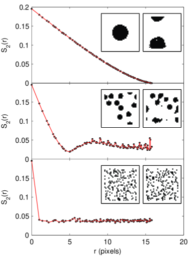
Examples of reconstructions of two-phase microstructures under periodic boundary conditions are given in Fig. 1. In the case of the single disk, the reconstructed microstructure is almost identical to the target, except for a translation (top portion of Fig. 1). In the case of the reconstruction of the hard disks (middle portion of Fig. 1), the characteristic size of the disks as well as the average distance between them is recovered. However, an exact reconstruction of the target configuration is not possible; spurious objects are also formed through the partial merging of neighboring disks. In the case of a realization of a Poisson point process (randomly coloring a pixel black according to a prescribed volume fraction), the reconstructed and the target microstructures might look superficially similar because they both appear to be random distributions of black pixels (bottom portion of Fig. 1). However, the two microstructures have very little in common if one is interested in the exact configurations of the pixels, although an excellent match is obtained between and . This illustrates the concept of non-trivial degeneracy Patterson (1939); Jiao et al. (2010a, b).
In a recent Letter Gommes et al. (2012), we presented a general theoretical framework for estimating quantitatively the structural degeneracy corresponding to any specified correlation function. This was achieved by mapping the problem to the estimation of a ground-state degeneracy through the use of Eq. (1). Here we provide a more comprehensive presentation of the methodology and analyses, including a quantitative characterization of the energy landscape associated with the reconstruction as well as a detailed derivation of the degeneracy metric. Moreover, we show that our results can be expressed in terms of the information content of the two-point correlation functions. Although the present work focuses on two-dimensional media in Euclidean space, our procedure can be applied in any space dimension and generalized to non-Euclidean spaces (e.g., compact and hyperbolic spaces).
The remainder of the paper is organized as follows. In Sec. II, we discuss the degeneracy of the two-point statistics for a variety of microstructures that are used as benchmarks throughout the rest of the paper. We consider successively small systems - for which all the configurations can be enumerated - intermediate systems - for which the degeneracy can be determined via a Monte Carlo method we presented elsewhere Gommes et al. (2012) - and large systems for which neither of the aforementioned two methods apply and one needs to use the reconstruction method. In Sec. III, we devise an analytical method, based on a random walk in configuration space, to characterize the energy landscape associated with reconstruction. In particular, we determine a characteristic energy profile for the basin of each ground state. In Sec. IV, we show that the ground-state degeneracy of reconstruction problems is related to the roughness of the energy landscape. We introduce a roughness metric that can be calculated from alone, and we show definitively that it is correlated with the microstructure degeneracy. In Sec. V, the degeneracy is expressed in terms of the information content of , and a formula is proposed relating the roughness metric to this information content. The practical usefulness of our results is discussed.
II The degeneracy of two-point statistics
II.1 Small-system-size microstructures: countable examples
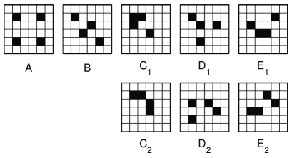
The present paper is restricted to two-phase digitized microstructures, which can be thought of as images with black pixels and white pixels. However, our analysis can be easily generalized to multiphase microstructures. We shall first consider the very small microstructures of Fig. 2 with . They will be analyzed in some detail and will serve as a benchmark for analytical methods applicable to larger and more complex microstructures.
For any finite microstructure it is always possible to refer to the pixels through a linear index, to , independently of the actual dimensionality. A finite microstructure is therefore completely characterized by a -dimensional vector, with components equal to when point is a black pixel, and otherwise. The two-point correlation function of the black phase is defined as the probability that two random pixels at a distance from one another are both black Torquato (2000). This can be written formally as
| (3) |
where takes the value if the distance between pixels and is , and otherwise. The quantity is defined as . In Eq. (3) the double sum counts the pairs of black pixels separated by a distance , and the pre-factor normalizes that count by the total number of pixel pairs at a distance from one another. The periodic boundary conditions are incorporated in the definition of the operator . We assume in the rest of the paper that the discretizing grid is uniform in the sense that is independent of .
The use of a discrete pixel grid is equivalent to a “quantizer” problem Torquato (2010), in which every point of the microstructure is quantized to the centroid of its closest pixel. The distances between pairs of points are therefore approximated by distances that are compatible with the grid. A square grid is used throughout the present paper. For finite-size systems, the quantization naturally introduces some grid-specific artifacts Jiao et al. (2008). However, the quantization error decreases and becomes zero in the limit of infinitely large microstructures.
The two-point correlation functions of the microstructures of Fig. 2 are given in Table 1 under the form . The quantity is equal to the number of pairs of points at distance from one another. Note that although configurations and are different, they have identical two-point characteristics. The same applies to and , as well as to and . A complete enumeration of all microstructures with shows that there is no other configuration with the same .
| 1 | 2 | 3 | |||||||
|---|---|---|---|---|---|---|---|---|---|
| 0 | 0 | 0 | 0 | 0 | 4 | 0 | 0 | 2 | |
| 0 | 1 | 0 | 4 | 0 | 0 | 0 | 0 | 1 | |
| 2 | 1 | 0 | 2 | 1 | 0 | 0 | 0 | 0 | |
| 0 | 1 | 2 | 0 | 1 | 0 | 2 | 0 | 0 | |
| 1 | 1 | 0 | 2 | 1 | 0 | 1 | 0 | 0 |
Configuration in Fig. 2 is uniquely defined by its two-point function, and therefore is only trivially degenerate. On grids with points the total number of translations is ; the number of rotations is , or , depending on the rotational symmetry of the configuration; and the number of mirror configurations is or , depending on its chirality. Due to the symmetry and chirality of configuration A, only translation contributes to its degeneracy, which is therefore . In the case of configuration , the two possible orientations contribute an extra factor 2, i.e. .
Configurations and are the ”Kite & Trapezoid” examples discussed in Refs. Patterson (1944); Jiao et al. (2010a, b), which are non-trivially degenerate. In this case, , where the factor 2 is the non-trivial contribution, and the factor 4 accounts for the possible orientations.
Configurations and are also non-trivially degenerate. Configuration is, however, chiral so it has to be counted twice. This leads to . Finally, non-trivially degenerate configurations and are both chiral. This leads to .
II.2 Intermediate-system-size microstructures: Monte Carlo analysis
The complete enumeration of degenerate microstructures is intractable for systems even barely larger than those represented in Fig. 2. In the present section, we discuss a Monte Carlo (MC) algorithm for estimating , which we introduced previously Gommes et al. (2012). It can be applied to larger systems.
The approach is based on a general MC algorithm for estimating the density of states (DOS) developed by Wang and Landau Wang and Landau (2001a, b) and further improved and analyzed by others Dayal et al. (2004); Zhou and Bhatt (2005); Belardinelli and Pereyra (2007). The algorithm has been applied to a host of problems in condensed matter physics Yamaguchi and Okabe (2001), in biophysics Rathore and de Pablo (2002), and in logic Ermon et al. . The DOS is defined as the number of states having energy equal to . The logarithm of is equal to the entropy calculated in the microcanonical ensemble associated with Eq. (1). The ground-state degeneracy is the value taken by for .
A canonical Monte Carlo simulation with transition probability given by Eq. (2) leads the system to visit any energy with a probability Metropolis et al. (1953). The algorithm of Wang and Landau is based on the observation that a transition probability of the form
| (4) |
would lead the system to visit all energies with equal probability. The density of states is, however, unknown so the algorithm is iterative.
The starting value is set to for all energies, and the system is let evolve according to Eq. (4), while updating an histogram . Each time an energy is visited the corresponding bin is updated, , and the estimated density of states is updated according to where is a numerical factor larger than 1. The evolution continues according to Eq. (4) with the updated value of . The evolution is stopped when a flat histogram is obtained. At this point, the histogram is reset to , is reduced to a value closer to 1, and the evolution starts over again. The entire procedure is repeated until becomes lower than a prescribed accuracy. Algorithmic details are provided in the Supplementary Material Sup .
The accuracy of the MC algorithm was tested by applying it to the microstructures of Fig. 2. The results are plotted in Fig. 3 in the form of cumulative DOS
| (5) |
The MC algorithm provides only to within an unknown multiplicative constant, which is determined by imposing to be equal to the total number of configurations . The latter is equal to the number of different ways in which black pixels can be chosen among a total of possible pixels, i.e.
| (6) |
The cumulative DOS plotted in Fig. 3 satisfies and .
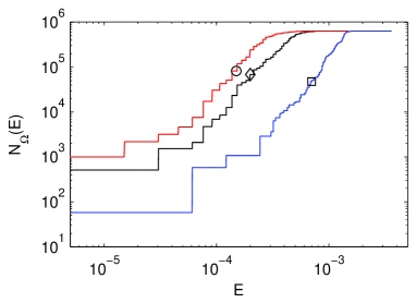
Three independent MC estimations have been calculated for each microstructure in Fig. 2, yielding three independent estimates of . The results are: for configuration A compared to the exact value ; for configuration B compared to ; for configuration C compared to ; for configuration D compared to ; and for configuration compared to . The exact values are those calculated in Sec. II.1 with . The agreement with the MC estimates is excellent.
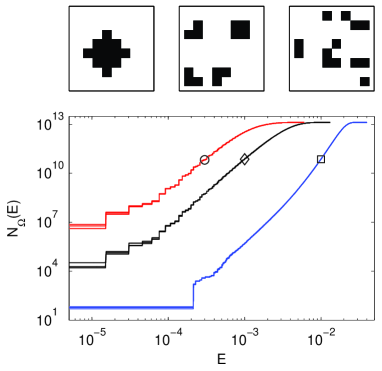
Figure 4 shows MC estimates of the density of states for larger microstructures, with on a grid. The microstructures are qualitatively similar to those of Fig. 1, namely a single disk, hard disks, and a Poisson point process, all under periodic boundary conditions. In the case of a single disk, the MC estimation provides the value , corresponding to the possible translations. This confirms that the disk is only trivially degenerate. By contrast, the value found for the Poisson point process is , which is orders of magnitude larger than any possible trivial contribution from translation and rotation. In the case of the hard disks, we find .
II.3 Large-system-size microstructures
The MC algorithm does not converge for systems larger than about pixels. With larger systems the criterion for flat histograms is rarely reached, even with as many as MC steps. Moreover, when flat histograms are indeed obtained, the estimated value of is much smaller than 1, which shows that the algorithm explores only a small fraction of the complete configuration space. These numerical difficulties are consistent with previous observations that flat-histogram algorithms have a convergence time that increases exponentially with system size Dayal et al. (2004).
It is therefore difficult to estimate the -degeneracy of systems as large as the one shown in Fig. 1, except in the particular case where the microstructure is only trivially degenerate. It has to be stressed that reconstructing exactly a degenerate microstructure is very unlikely. Therefore, whenever a reconstruction leads to a translated, rotated, and inverterted version of the target, this can be considered as very strong evidence that the microstructure is only trivially degenerate. In the remainder of the paper, we shall refer to a microstructure as being non-degenerate, whenever it has only a trivial degeneracy.
In continuous Euclidean space under periodic boundary conditions, an example of non-degenerate microstructure is provided by the single sphere (composed of a large number of pixels). This results from the observation that is equal to volume fraction of the solid phase and that the negative slope of for is proportional to its surface area Debye et al. (1957). A sphere is non-degenerate because it is the microstructure that realizes the lowest possible surface area for a given volume fraction: the two-point correlation function of any microstructure other than a single sphere would have a larger slope at the origin, which would result in a positive energy according to Eq. (1).
This observation can be expressed in a way that generalizes to discrete microstructures: for a given number of black pixels , a single sphere is non-degenerate because it is the microstructure that realizes the largest value of , where is a very small distance. Similarly, any configuration with other than the disk of Fig. 4 has a smaller value of , where it is to be recalled that is the number of pairs of points with distance . The same applies to configuration of Fig. 2, which is not a disk: that particular microstructure is non-degenerate because any other configuration with has a smaller value of . The origin of the degeneracy of hard-disk systems is touched on in Sec. VI.
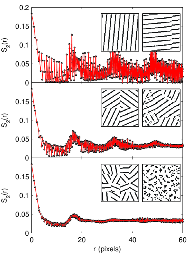
The analysis of non-degeneracy in terms of extremal values of leads to non-intuitive results. When microstructures are defined on a grid, distances and orientations are not independent: for instance, a pair of points at a distance from one another is necessarily oriented at 45° with respect to both axes. A very anisotropic microstructure such as the crystal on the top of Fig. 5 minimizes for a set of distances corresponding to orientations orthogonal to the stripes. The figure clearly shows that vanishes for a set of well-defined distances. It should therefore not be surprising that such a highly anisotropic microstructure is non-degenerate. The non-degeneracy of the crystal is confirmed by the fact that the reconstructed microstructure in Fig. 5 is a translated and rotated copy of the target. The vertical discontinuity in the middle of the reconstruction results simply from the target not having the same periodicity as the box.
When a large crystal in a periodic box is split into a collection of randomly oriented smaller crystallites (Fig. 5 middle and bottom rows), its anisotropy is reduced and there are no longer values of at which is extremal. Accordingly the reconstruction becomes less accurate, which means that the microstructure becomes more degenerate. A more quantitative analysis of this issue is provided in Sec. V.
III Characterization of the Energy Landscape
III.1 The Structure of Configuration Space
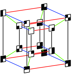
The complete configuration space of two-phase microstructures with pixels is the set of vertices of an -dimensional hypercube Gommes et al. (2012). This results from the properties of the indicator vector, , which can take only values and . Moving along a given -dimensional direction (along an edge of the hypercube) is equivalent to interchanging a white (black) with a black (white) pixel. In the example of Fig. 6, any movement along the fourth dimension (joining the outer and inner cubes) corresponds to changing the upper-left pixel.
In the situation relevant to reconstruction, not all the vertices of the hypercube are accessible because the number of black pixels is kept constant, i.e.
| (7) |
which means that all realizable microstructures lie on the intersection of the hypercube with a hyperplane. Once a target correlation function is specified, each vertex is assigned an energy through Eq. (1).
What we refer to as the energy landscape is the set of values taken by the energy functional on the vertices of the -dimensional hyperplane. A reconstruction consists in exploring the energy landscape until a vertex is found with . The DOS determined in section II.2 is the number of vertices having a given energy . The problem we address in this section is that of the spatial variability of in configuration space . This analysis is motivated by the observation, in many fields of physics, that systems with large ground-state degeneracies generally have a rough energy landscape Wales et al. (1998); Debenedetti and Stillinger (2001). If we can characterize the roughness of the energy landscape in terms of we can estimate the ground-state degeneracy .
In order to characterize the spatial variability of in configuration space, it is necessary to define a distance. A natural choice is the Hamming distance, which counts the number of edges between any two vertices. The Hamming distance within the hyperplane defined by Eq. (7) takes only even values. The distance between two microstructures and is therefore defined as half the Hamming distance
| (8) |
where and are the indicator vectors. In real space, this distance is the smallest number of Monte-Carlo-like black pixel displacements that are required to pass from to . The largest possible distance is when the two microstructures have no pixel in common 222We assume throughout the paper that black pixels are fewer than white pixels, which does not limit the generality of the analysis..
III.2 Exploring the Energy Landscape with a Random Walk
The energy landscape can be characterized analytically through a random walk in configuration space. This is illustrated in Fig. 7. Starting from a ground state of a reconstruction problem, with , the system moves randomly to any configuration at Hamming distance from the current configuration. This is equivalent to a standard Metropolis Monte Carlo with [see Eq. (2)]. When the number of moves increases, the random walk explores the configuration space over increasingly large Hamming distances from the starting ground state.
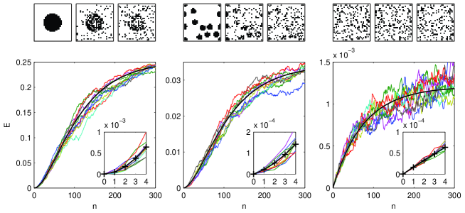
The rate at which the average energy visited by the random walk increases with the number of moves characterizes the energy landscape of a given reconstruction problem. In the examples of Fig. 7, the energy curve of the Poisson point process is steeper than that of the single disk, which suggests smaller basins. We now proceed to analytically calculate the values of as a function of the characteristics of the starting ground state.
The only a priori information about the ground states of a given reconstruction problem is their one-point and two-point characteristics: and . The other characteristics, in particular the higher-order correlation functions, may differ significantly from one ground state to another. Let us assume for now that the starting ground state of the random walk is perfectly known through its indicator vector .
Instead of using , it is convenient to use the equivalent autocovariance defined as
| (9) |
where is the fraction of black pixels. The average energy after random moves can be written in terms of as
| (10) |
where we have used the notations , which is associated with the ground state, and for any average value at step . At each step of the random walk there are possible moves, so that the total number of possible walks of length is : the averages are calculated over all these possible paths. We now calculate successively and , which are required to calculate and through Eq. (10).
When a black pixel is moved to position previously occupied by a white pixel, the indicator vector becomes
| (11) |
where is the Kronecker delta function. Using the definition of , Eq. (3), the autocovariance is then found to become
| (12) |
for that particular move. The average value of is then simply calculated as
| (13) |
where the factor accounts for the fact that and are uniformly distributed over the black and white phases, respectively.
Combining Eqs. (III.2) and (13), the average autocovariance after a single random move is found to be
| (14) |
with . In Eq. (14) a term of the order of has been neglected, which is justified for large values of . The complete equation can be found in the Supplementary Material Sup . Equation (14) is valid only for . The value for depends only on the fraction of black pixels , , and it is therefore a constant during the random walk.
Because each random move is independent from the previous one, the analysis leading to Eq. (14) can be repeated in an iterative way. Taking into account that the starting two-point function is , this leads to the following simple result
| (15) |
In the course of the random walk, the average two-point function therefore converges towards that of a Poisson point process Serra (1982); Torquato (2000) with for all . The convergence is exponential in the number of random moves and it occurs in about moves.
The determination of proceeds along the same lines, but it is more involved; the details can be found in the Supplementary Material Sup . When the expression obtained for is introduced in Eq. (10), the value of the average energy takes eventually the form
| (16) |
where , , and are constants that characterize the starting ground state. The constants and depend only on and
| (17) |
and has the same meaning as in Eq. (14).
The constants and depend only on two-point characteristics of the ground states. They are written as
| (18) |
and
| (19) |
where the sum is over all the distances that are used in the definition of the energy. As a consequence of Eq. (III.2), is the value towards which converges for large values of . Since the random walk is ergodic, any configuration has the same probability of being visited in the long run. Therefore, is the average energy calculated over the entire configuration space, which we refer to hereafter simply as .
The main contribution to is , which is small for disordered microstructures. This term vanishes in the extreme case of a Poisson point process for which the only contribution left is of order , according to Eq. (19). The shifting of the average energy towards lower values with increasing disorder is clear in Figs. 4 and 7.
The other two constants, and , in the expression of depend on more than the two-point function of the ground state. They are given by
| (20) | |||||
and
| (21) | |||||
where the functions and are defined as
| (22) |
and
| (23) |
We postpone to Sec. IV the detailed discussion of the structural meaning of and . We should only mention here that can be expressed in terms of and that it is therefore common to all ground states (see the Supplementary Material Sup ). By contrast, depends on three-point statistics and may differ from one ground state to another.
The black lines in Fig. 7 have been obtained from Eq. (III.2) with the constants to evaluated at the starting ground state. The analysis captures the essential features of the random walk, in particular the steepness of the versus curves.
An important quantity for the rest of the analysis is the average energy of all configurations at Hamming distance from the ground state. Setting in Eq. (III.2) and neglecting terms of the order of , leads to
| (24) |
The first two contributions are global characteristics of the configuration space, which depend only on and are therefore common to all ground states. By contrast, the contribution from may a priori differ significantly from one ground state to another. We discuss this point in detail in Sec. IV.
III.3 The Energy Profiles of Individual Basins
The average energies visited after exactly random moves is strictly a property of the random walk, not only of the energy landscape. The aim of the present section is to use Eq. (III.2) to calculate the average energy of all microstructures at a given Hamming distance from a given ground state.
A random walk of length can reach any microstructure at Hamming distance from the ground state. Let us call a -state a microstructure at distance from the ground state, and the fraction of all the random walks of length that end on a -state. The average energy of all -states is related to through
| (25) |
If the values of were known, this relation could in principle be inverted to estimate starting from Eq. (III.2).
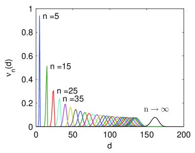
The distribution can be obtained by noticing that the random walk is a Markov process, and by calculating the transition probabilities between various -states. In real space, the Hamming distance is the minimum number of pixel displacements that is necessary to make the state identical to the ground state. Therefore, in a -state, the black phase is identical to the ground state but for holes, and the white phase is identical to the ground state but for extra pixels. Starting from an -state at step , there are ways to reach a -state at step . These correspond to the number of different ways to take one of the extra pixels and place it into one of the holes. The transition probability is therefore
| (26) |
where the denominator is the total number of possible moves. There are different ways to reach another -state. These correspond to the different ways of moving the holes within the black phase, plus the different ways of moving the extra pixels within the white phase. The transition probability is therefore
| (27) |
Finally, there are different ways of reaching a -state, which correspond to the different ways of taking a black pixel and putting it in the white phase. This leads to
| (28) |
The three transition probabilities add up to , which proves that all possibilities have been considered.
The enumerated probabilities define a tridiagonal transition matrix of size , with elements . The explicit form of is given in the Supplementary Material Sup . Writing the values in a vector as enables us to write . The general solution is therefore
| (29) |
where is the trivial distribution of Hamming distances in the ground state.
The particular evolution of for and is shown in Fig. 8. These values are relevant to Fig. 7. For small values of , the distribution is centered on the value . For large values of , however, converges towards an equilibrium distribution. It is useful to note that although all states are accessible to the random walk after moves, the energy continues to changes for larger values of (see Fig. 7) because the convergence of is asymptotic.

Using the known values of and of , Eq. (25) can be inverted for , yielding the values of . The procedure is illustrated in Fig. 9 for the small-system-size configurations of Fig. 2. The results are plotted in the normalized form , which we refer to as the energy profiles.
The energy profiles describe quantitatively the average energy landscape surrounding any particular ground state. They are all initially increasing curves that start from and reach values close to . The average energy for is equal to , as calculated from Eq. (24). For large Hamming distances the energy decreases again because microstructures with large can be thought of as negative imprints of the ground state: for the points that were occupied by black pixels in the ground state are all occupied by white pixels.
Figure 10 shows the energy profiles of the single disk, the hard disks, and the Poisson point process of Fig. 4. When plotted on logarithmic scales (insets), the profiles are seen to satisfy a power law of the type
| (30) |
for small values of . When the resolution is increased - i.e. increasing from to and while keeping constant - the profiles are shifted vertically (insets) but the exponent of the power law persists. In the case of the reconstruction of the single disk, the exponent is close to (), and for the reconstruction of the Poisson point process the exponent is close to (). The energy profile of the hard disks is not a pure power law: the exponent is that of a single disk for large Hamming distances and that of a Poisson point process for shorter distances.
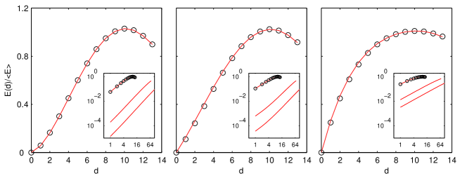
The different exponents for the Poisson point process and for the single disk hint at a qualitative difference that can be understood with the hole and extra pixel interpretation of Hamming distance . In the case of the Poisson point process, the energy is proportional to . This means that any hole added to the ground state contributes additively to the energy, which points to the absence of effective pixel-pixel interaction energy. By contrast, the quadratic behavior for the single disk points to a collective contribution of the pixels to the overall energy, which can be considered as the signature of a structure.
IV Energy Roughness as a Proxy for Ground-State Degeneracy
When comparing the energy profiles in Figs. 9 and 10 with the densities of states in Figs. 3 and 4, a striking correlation appears between the sizes of the basins and the ground-state degeneracy . We observe that the smaller the basin, the more degenerate the reconstruction. This observation is consistent with the one that large ground-state degeneracies are generally associated with rough energy landscapes Wales et al. (1998); Debenedetti and Stillinger (2001).
However, a major difference between the energy profiles and the ground-state degeneracy is that the latter is a global characteristic of the reconstruction problem but the former are specific to given ground states. For example, in the case of configuration of Fig. 2, the ground states (the Kite) and (the Trapezoid) have slightly different energy profiles (Fig. 9). The main purpose of the present section is to provide an approximation for the energy profile, common to all ground states, which can be calculated from alone.
To understand how the energy profiles depend on the particular ground state, it is necessary to analyze the structural meaning of functions and defined by Eqs. (22) and (23). We show in the Supplementary Material Sup that can be expressed in terms of the two-point function as
| (31) |
where is a characteristic of the grid and of the boundary conditions. By definition, all ground states have identical two-point statistics. The contribution of to the energy profile is therefore common to all ground states. By contrast, it results from Eq. (23) that is a sum of terms of the type
| (32) |
which incorporate three-point statistics. Accordingly, the contribution of to the energy profile may differ significantly from one ground state to another.
As a consequence of Eq. (32), the pixel configurations that contribute to are isosceles triangles with apex and side-length . In the case of configuration of Fig. 2, the Kite () has two such triangles, one with and the other with . On the contrary there is no isosceles triangle in the Trapezoid (). It therefore results from Eq. (24) that is larger for than for , in agreement with Fig. 9.
The energy profiles of and are identical although these two ground states are different. This originates in the fact that in both ground states, there is an isosceles triangle of side and another one of side . The same explanation applies to and . In both ground states there is a single isosceles triangle with .
Despite these differences between and , the two functions have a strong similarity which can be put in evidence by the following probabilistic interpretation. Consider the set of all pixels at distance from a given pixel , which we refer to as the ring centered on . The fraction of black pixels in the ring can be written as
| (33) |
When is chosen randomly among all pixels (black and white) is a random variable having average value . Equation (22) shows that is the variance of . The function can therefore be thought of as a generalized coarseness Lu and Torquato (1990).
From this probabilistic perspective, the meaning of is equivalent to , only the central pixel is not distributed randomly over the entire space but only over the black pixels. In this case, the average of is the conditional probability that a pixel of the ring is black, given that the central pixel is black too, i.e. . From Eq. (23), one sees that is the variance of when the central pixel is randomly distributed over the black phase. The function can therefore be thought of as a conditional coarseness.
For small radii , the values taken by on the ring are highly correlated with the value in the center, which implies . For large radii, the values on the ring and in the center are not correlated at all and therefore . An example of and , calculated on the realization of a hard-disk system is given in Fig. 11.
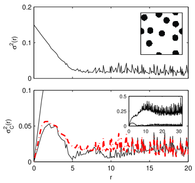
The similarity of the probabilistic interpretations of and of , and their strict mathematical equality for large values of , suggest that it should be possible to find an approximation of in terms of two-point functions only. This would enable us to estimate a single approximate energy profile that would depend only on . That profile would therefore be common to all ground states of a given reconstruction problem.
To find such an approximation, we observe that the terms between braces in the definitions of and are identical and that they are all positive (see Eqs (22) and (23)). However, there are fewer terms in Eq. (23) because can be equal to . One has therefore
| (34) |
which leads to the following upper bound for :
| (35) |
which depends only on two-point statistics.
The inset of Fig. 11 compares to in the particular case of a hard-disk microstructure. The upper bound is a good approximation of only for very small . We therefore propose the following approximation for
| (36) |
which is practically equal to for large , as it should. Fig. 11 shows that is a fair approximation of at all radii.
Using in place of enables us to calculate a single energy profile, based on alone. The red curves in Figs. 9 and 10 have been calculated in that way: was calculated rigorously from the target through Eq. (31), and was approximated by Eq. (36). In the case of the larger microstructure shown in the insets of Fig. 10, the approximate profiles are indistinguishable from the exact profiles on the scale of the figure.
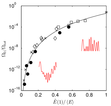
Using Eq. (36) it is possible to estimate a single metric to characterize globally the roughness of the energy landscape. We propose the ratio
| (37) |
where the tilde highlights the fact that is estimated through the approximation . The quantity is the average energy of all microstructures at distance from the ground state. Because the ground states have zero energy, can be thought of as a Laplacian in configuration space . The ratio is therefore a dimensionless measure of the total curvature of the energy surface in the vicinity of any ground state. It has to be stressed that is calculated from alone, and that it is therefore not specific to any particular ground state.
Figure 12 shows the quantitative relation between and the normalized ground-state degeneracy for a variety of microstructures defined on a grid. The microstructures used for the figure are available in the Supplementary Material Sup : they comprise both non-degenerate disk-like objects and highly degenerate realizations of Poisson point processes. The ground-state degeneracy of the latter was estimated via the MC algorithm. The quantity is found to be highly correlated with over more than 14 orders of magnitude.
When passing from small to large values of , the energy landscape changes qualitatively in the way suggested by the insets of Fig. 12. For low values of , the energy landscape has an overall funnel structure, with low energy barriers, which makes it well suited for optimization problems. By contrast, for large values of , the landscape is very rough with a large ground-state degeneracy. It is, however, interesting to note that the rightmost point in Fig. 12 is obtained for a system with having thus only a trivial degeneracy. The corresponding energy landscape is extremely rough because any possible energy can be found at a Hamming distance as short as from the ground state, but the total number of configurations is also extremely small.
The data referred to as disks in Fig. 12 is a collection of non-degenerate microstructures with increasing values of . When increasing , the roughness decreases but the degeneracy remains equal to its trivial translation contribution . It is noteworthy that the values of of these non-degenerate microstructures span the same curve as the realizations of Poisson point processes, for which has a huge non-trivial contribution.
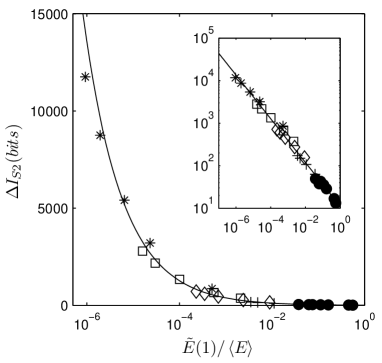
The microstructures considered in Fig. 12 were limited to grids, which size limit is imposed by the convergence of the MC algorithm. However, the fact that the -versus- curve does not discriminate trivial from non-trivial degeneracy should not be limited to small microstructures. This assumption enables us to extend the curve to larger microstructures by using disks of increasing sizes , on grids with increasing sizes , for which the degeneracy is known to be exactly . This was done in Fig. 13. The degeneracy is plotted in the form of for reasons that will be explained in next section. The inset of the figure shows that disks of all sizes and on all grids span a single curve which obeys approximately a power law.
V Degeneracy Analysis Using an Information-Theoretic Formulation
The degeneracy can be analyzed in terms of the information content associated with a given two-point function . Indeed, if a reconstruction problem is non-degenerate, the two-point correlation function is a complete characterization of the microstructure. By contrast, in the case of a large degeneracy the correlation function contains a relatively small amount of microstructural information.
This idea can be made quantitative by borrowing concepts from information theory Cover and Thomas (1991); Berut et al. (2012). In that context, a given microstructure is considered to be the outcome of a random process. More specifically, if nothing is known other than the total number of pixels , then specifying a given microstructure is equivalent to drawing it out of the complete configuration space. Any microstructure is therefore an event having probability . The self-information (or so-called surprisal) associated with such an event is
| (38) |
The use of a base 2 logarithm ensures that the self-information is expressed in units of bits. The self-information can be used as a quantitative measure for the information content of the realization of an event. In this particular case, the value is bits, i.e., 1 bit per pixel, which is quite consistent.
| Microstructure | ||||||
|---|---|---|---|---|---|---|
| Single disk | 1024 | 200 | 0.29 | 0.81 | 1.10 | |
| Hard disks | 1024 | 200 | 0.29 | 0.48 | 0.77 | |
| Poisson point process | 1024 | 200 | 0.29 | 0.10 | 0.39 | |
| Crystal | 16384 | 3000 | 0.31 | 0.61 | 0.93 | |
| Polycrystal 1 | 16384 | 3000 | 0.31 | 0.32 | 0.63 | |
| Polycrystal 2 | 16384 | 3000 | 0.31 | 0.22 | 0.53 |
If the number of black pixels is known, a microstructure is no longer a draw out of , but rather out of . This implies that the self-information is reduced by a quantity
| (39) |
which can be thought of as the amount of information contained in specifying the value of , compared to knowing merely the system size. We refer to as the information content of the one-point statistics. The quantity depends on the particular value of . It is equal to for and for . In both cases specifying is a complete description of the microstructure, since in those cases the system is either completely black or completely white. By contrast, is minimum for , because this particular value maximizes .
The same reasoning can be applied to quantify the information content of . Once is given, a particular microstructure is drawn out of possibilities, and no longer . This suggests defining the quantity
| (40) |
to measure the information content of , in addition to knowing .
Note that the information content of the one-point and two-point statistics can be understood in terms of configurational entropies corresponding to different definitions of the macrostate of the system. In the case of the one-point information, the macrostate is specified via the value of , which results in an entropy . Similarly, if is used to define the macrostate, the entropy becomes . The information content is equal to the entropy reduction that results from incorporating in the definition of the macrostate of the system.
The analysis of Sec. IV suggests that can be accurately calculated from alone. This is the significance of Fig. 13. The inset of the figure shows that the dependency is a power-law of the type
| (41) |
where the numerical coefficients have been obtained by a least-square fit. It has to be stressed here that the roughness metric is calculated from alone. Therefore, Eq. (41) provides a practical means to estimate in any experimental context where the only information about the system is its correlation function .
For a reconstruction to be accurate, the total information available in the form of one-point and two-point statistics, has to be bits. Therefore, the utility of and is best illustrated by normalizing them by and defining the following fractional information contents and , which take values between 0 and 1. A reconstruction is accurate whenever the sum is close to one. Table 2 analyzes the reconstruction examples of Figs. 1 and 5 along these directions.
The three microstructures of Fig. 1 all have black pixels on a grid with a total of pixels. In this case, one estimates through Eq. (39) that the one-point information is . The two-point information for the various microstructures was calculated from the roughness metric through Eq. (41) and the corresponding values of are reported in Table II. In the case of the single disk, the total information content of and is close to 1, which means that a perfect reconstruction is possible. The fact that the value is slightly larger than 1 results from the limited accuracy of Eq. (41). In the case of the Poisson point process, the total information available amounts to only 39% of the information required for the reconstruction: the reconstruction is therefore impossible.
The case of the hard disks is not so clear-cut: the reconstruction captures many structural characteristics of the target (Fig. 1) although only 77% of the information is available (Table 2). This seems to suggest that a fair reconstruction may be possible with about 20% of missing structural information.
The information-theoretic analysis of the polycrystal reconstructions of Fig. 5 proceeds in the same way. In the case of the single crystal, 93% of the information is (see Table 2), which is consistent with the good quality of the reconstruction. For decreasing crystallite sizes, the amount of information decreases. In the case of the smallest crystallites, the amount of information is only about 50 % and the reconstruction is expectedly inaccurate.
The consistency of the information analysis of the single disk reconstruction was expected because Fig. 13 and Eq. (41) are based on disks of various sizes. The validity of Eq. (41) for microstructures other than disks is established only for very small systems, for which the MC algorithm could be used (Fig. 12). The fact the present analysis enables us to predict the non-degeneracy of the crystal reconstruction strongly supports the generality of Eq. (41).
VI Discussion and Conclusions
Throughout the paper, we have discussed several cases of trivially and non-trivially degenerate microstructures. We have argued that the geometrical features that contribute to decreasing the non-trivial contribution to are those that lead to extremal values of for given values of . This is notably the case for a single disk under periodic boundary conditions, which is the microstructure that maximizes for sufficiently small ’s. The crystal configuration shown in Fig. 5 is non-degenerate for similar reasons: because of its anisotropy, that microstructure achieves extremal values of for many different values of . The opposite situation is that of a Poisson point processes, for which takes values close to the average value for all . This leads to a huge degeneracy (configurational entropy) because none of the values of is close to being extremal.
It is interesting to note that the single disk within a periodic box can be thought of as a dilute distribution of disks in all of Euclidean space when the infinite number of periodically replicated cells are considered. In the case of impenetrable disks at arbitrary density, it is noteworthy that can be exactly expressed in terms of a one-body or low-density term (which contains the same shape and surface area information as in the dilute regime) and a single higher-order two-body term involving pair statistics Torquato (2000); Torquato and Stell (1985). It is therefore the latter term that is responsible for the degeneracy of such configurations for arbitrary densities.
The trivial contribution to the degeneracy depends on the particular rotational symmetry and chirality of the microstructure, but it is always of the order of total number of pixels in the grid . By contrast, the non-trivial contribution to the degeneracy can be significantly larger. The Monte Carlo estimation of shows that even a modestly sized Poisson point process can have a degeneracy as large as (see Fig. 4). This value is expected to increase exponentially with the size of the system because any possible -preserving pixel displacement contributes multiplicatively to .
In order to quantitatively address the question of the degeneracy corresponding to any specified correlation function, we have mapped it to the determination of a ground-state degeneracy. This mapping led us to two breakthroughs. First, we now can calculate for the first time the density of states for reconstruction problems via a Monte Carlo algorithm, and in particular to determine the values of for a few benchmark systems. Second, we built on the general observation throughout physics that large ground-state degeneracies are generally associated with rough energy landscapes, which enabled us to use the roughness of the energy landscape as a proxy for the microstructural degeneracy.
A natural metric for the roughness of the energy landscape is the total curvature of the energy surface, evaluated at the ground-states. Using a random walk in configuration space (see Fig. 7), we derived an analytic expression for the total energy-surface curvature in the form of , which can be calculated in terms of alone. The Monte Carlo analysis confirms that is indeed highly correlated with the degeneracy of a reconstruction problem, independently of the type or microstructure considered (Fig. 12). It has to be noted that the roughness metric is consistent with the intuitive analysis of degeneracy in terms of extremal values of . Indeed, the main contribution to the denominator is , so that any value of larger or smaller than contributes to decreasing the roughness metric, and hence the degeneracy.
A counterintuitive result of the present study is that the distinction between trivial and non-trivial degeneracy is irrelevant in configuration space . In particular, the quantitative relationship found between and the roughness metric does not discriminate the two types of degeneracy. This enabled us to use trivially-degenerate microstructures to generate a single calibration relation for as a function of . That relation applies to a large variety of microstructures of sizes much larger than those analyzable by the Monte Carlo method (see Fig. 13).
We should point out that although the examples discussed in the present work are all two-dimensional microstructures, the same methodology can be applied in any space dimension. It is indeed noteworthy that Eq. (24) and the approximation Eq. (36) are valid in any space dimension. As a consequence, the roughness metric of any higher-dimensional microstructure can be calculated easily from its correlation function alone. Moreover, the observation that we make that the relation between the roughness metric and the ground-state degeneracy does not discriminate trivial from non-trivial degeneracy is also expected to hold in any space dimension. Therefore, higher-dimensional trivially-degenerate microstructures (e.g. hyperspheres) can be used to produce a relation equivalent to Eq. (41) or Fig. 13 in any space dimension.
It is also noteworthy that our analytical results do not assume Euclidean space: the only restriction is that should be independent of , where is the operator used to define through Eq. (3). Therefore, the mathematical expression of the roughness metric is valid in hyperbolic and spherical spaces as well as in any dimension. However, the relationship between the degeneracy (configurational entropy) and the roughness metric is expected to be space- and dimension-dependent.
The use of information-theoretic concepts allows our methods to be easily applied in practice. As mentioned in the introduction, two-point correlation functions are often the only data available experimentally for in situ studies with a nanometer resolution, notably through small-angle scattering measurements Svergun (1999); Svergun et al. (2001); Beale et al. (2006). The question of the structural ambiguity of small-angle scattering patterns is an old one Patterson (1939); Volkov and Svergun (2003); Gommes and Roberts (2008), but the recent development of very intense X-ray sources Bostedt et al. (2012) has ignited a very lively debate about the possibility of reconstructing nanometer-scale objects from scattering patterns Reich (2011). Our analysis provides a novel and very general approach to address this type of question: An accurate reconstruction is possible whenever the amount of information is close to one. The examples that we have discussed suggest that a relatively accurate reconstruction is possible with up to 20% missing information, but it is premature to formulate any general rule.
It has to be stressed that, although the present work is based on the reconstruction of microstructures defined on a grid with exact distances, the results apply unchanged to the discrete reconstruction of microstructures starting from experimental (i.e., continuous) correlation functions. Correlation functions of the type of the monocrystal (Fig. 5) are unrealistic in an experimental context. However, the general relation between and still holds. The only difference is that experimental correlation functions of disordered systems are generally of the polycrystal type, with very small crystallites. Except in some exceptional cases, it is therefore expected that experimental correlation functions with no orientation information should be highly degenerate.
The domain of applications of our results is not limited to scattering. Other applications can notably be found in the field of computer vision for texture recognition. A texture with low degeneracy can in principle be discriminated robustly based on two-point statistics alone, which would make slower three-point characterizations unnecessary Yellott (1993).
Besides applications, information-theoretic concepts are also useful conceptually. It is very natural that a reconstruction be possible whenever the information content of the available data is equal to the amount of information required, i.e. bits where is the total number of pixels. In the cases we considered, the information came in the form of one-point statistics and of two-point statistics . However, the approach could be generalized naturally to higher-order statistics Matheron (1967); Torquato and Stell (1982, 1983); Torquato et al. (1988). Quite generally, a successful reconstruction would require all correlations to be considered up to the th order, with satisfying
| (42) |
where is the information contained in n-point correlation function in addition to .
There is some evidence supporting the view that does not contain significant information in addition to Aubert and Jeulin (2000); Jiao et al. (2009). In the present context this suggests that the series in Eq. (42) converges slowly. The approach could be further generalized to other types of statistical descriptors including lineal statistics Méring and Tchoubar (1968); Torquato and Lu (1993), pore-size functions Serra (1982); Torquato (2000), and cluster correlation functions Torquato and Stell (1985); Jiao et al. (2009).
We stress that the present work has numerous ramifications in materials sciences and beyond. For instance, an important question concerns the realizability of two-point correlation functions Torquato (2006); Quintanilla (2008). It would be interesting to explore whether new necessary conditions for the realizability of can be obtained by expressing that the information content (in bits) cannot exceed the total number of pixels in the microstructure.
Last but not least, other applications can be found in physics. Indeed, the Hamiltonian of any system with pairwise additive energy can be written as
| (43) |
where is the pair interaction potential. It results from Eq. (43) that systems with identical necessarily have the same energy. Therefore the degeneracy calculated from is a lower bound for the physical ground-state degeneracy of any system with pairwise interaction energy. This includes systems such as frustrated Ising models for which the ground-state degeneracy is not trivial Parisi (2006). Another fascinating field of application is that of quasi-crystalline microstructures Levine and Steinhardt (1984), the degeneracy of which could be analyzed with the general results obtained in the present study.
¿From a methodological point of view, the general approach we have developed may be valuable in the manifold of fields where complex energy landscapes have to be characterized. These include protein folding Chavez et al. (2004), complex chemical reactions Wales et al. (1998), phase equilibria in disordered porous materials Puibasset (2010); Gommes (2012), and glass transitions Debenedetti and Stillinger (2001). We hope to investigate some of these aspects in future work.
Acknowledgements.
C.J.G. acknowledges support from the Fonds de la Recherche Scientifique (F.R.S.-FNRS, Belgium) and from the Patrimoine de l’Université de Liège; S.T. and Y.J. were supported by the Office of Basic Energy Science, Division of Materials Science and Engineering under Award DE-FG02-04-ER46108.References
- Zallen (1983) R. Zallen, The Physics of Amorphous Solids (Wiley, New York, 1983).
- Proakis and Manolakis (2006) J. G. Proakis and D. K. Manolakis, Digital Signal Processing, 4th ed. (Prentice Hall, 2006).
- Serra (1982) J. Serra, Image Analysis and Mathematical Morphology, Vol. 1 (Academic Press, London, 1982).
- Chandler (1987) D. Chandler, Introduction to Modern Statistical Mechanics (Oxford University Press, New York, 1987).
- Chilès and Delfiner (1999) J.-P. Chilès and P. Delfiner, Geostatistics: Modeling Spatial Uncertainty (Wiley, New York, 1999).
- Matheron (1967) G. Matheron, Elements pour une Théorie des Milieux Poreux (Masson, Paris, 1967).
- Torquato (2000) S. Torquato, Random Heterogeneous Materials (Springer, New York, 2000).
- Sahimi (2003) M. Sahimi, Heterogeneous Materials I: Linear Transport and Optical Properties, Vol. 1 (Springer, New York, 2003).
- Glatter and Kratky (1982) O. Glatter and O. Kratky, Small Angle X-ray Scattering (Academic Press, New York, 1982).
- Feigin and Svergun (1987) L. A. Feigin and D. I. Svergun, Structure Analysis by Small-Angle X-Ray and Neutron Scattering (Springer, Berlin, 1987).
- Filipponi et al. (1995) A. Filipponi, A. DiCicco, and C. R. Natoli, Phys. Rev. B 52, 15122 (1995).
- Drake et al. (1991) J. M. Drake, J. Klafter, and P. Levitz, Science 251, 1574 (1991).
- Barral et al. (1992) G. A. Barral, L. Frydman, and G. C. Chingas, Science 255, 714 (1992).
- Gommes et al. (2007) C. J. Gommes, J. P. Pirard, and S. Blacher, J. Microsc. 226, 156 (2007).
- Gommes et al. (2010) C. J. Gommes, H. Friedrich, P. E. de Jongh, and K. P. de Jong, Acta Mater. 58, 770 (2010).
- Svergun (1999) D. I. Svergun, Biophys. J. 76, 2879 (1999).
- Svergun et al. (2001) D. I. Svergun, M. V. Petoukhov, and M. H. J. Koch, Biophys. J. 80, 2946 (2001).
- Beale et al. (2006) A. M. Beale, A. M. J. van der Eerden, S. D. M. Jacques, O. Leynaud, M. G. O’Brien, F. Meneau, S. Nikitenko, W. Bras, and B. M. Weckhuysen, J. Am. Chem. Soc. 128, 12386 (2006).
- Gommes and Roberts (2008) C. J. Gommes and A. P. Roberts, Phys. Rev. E 77, 041409 (2008).
- Patterson (1944) A. L. Patterson, Phys. Rev. 65, 195 (1944).
- Yeong and Torquato (1998) C. L. Y. Yeong and S. Torquato, Phys. Rev. E 57, 495 (1998).
- Aubert and Jeulin (2000) A. Aubert and D. Jeulin, Patt. Rec. 33, 1083 (2000).
- Sheehan and Torquato (2001) N. Sheehan and S. Torquato, J. Appl. Phys. 89, 53 (2001).
- Hansen et al. (2005) B. L. Hansen, B. L. Adams, M. E. Lyon, and A. Henrie, J. Comp.-Aided Mater. Design 10, 163 (2005).
- Fullwood et al. (2008) D. T. Fullwood, S. R. Niezgoda, and S. R. Kalidindi, Acta Mater. 56, 942 (2008).
- Jiao et al. (2010a) Y. Jiao, F. H. Stillinger, and S. Torquato, Phys. Rev. E 81, 011105 (2010a).
- Jiao et al. (2010b) Y. Jiao, F. H. Stillinger, and S. Torquato, Phys. Rev. E 82, 011106 (2010b).
- Berthier and Tarjus (2011) L. Berthier and G. Tarjus, J. Chem. Phys. 134, 214503 (2011).
- Debye et al. (1957) P. Debye, H. R. Anderson, and H. Brumberger, J. Appl. Phys. 28, 679 (1957).
- Ciccariello (1983) S. Ciccariello, Phys. Rev. B 28, 4301 (1983).
- Patterson (1939) A. L. Patterson, Nature 143, 939 (1939).
- Hauptman (1986) H. Hauptman, Science 233, 178 (1986).
- Chubb and Yellott (2000) C. Chubb and J. I. Yellott, Vis. Res. 40, 485 (2000).
- Rozman and Utz (2001) M. G. Rozman and M. Utz, Phys. Rev. E 63, 066701 (2001).
- Rozman and Utz (2002) M. G. Rozman and M. Utz, Phys. Rev. Lett. 89, 135501 (2002).
- Note (1) In the case of the direct method of crystallography, the absolute orientation is generally lost through the measurement of a powder scattering pattern. The orientation with respect to the unit cell, however, is known from the indexing of the Bragg peaks.
- Gagalowicz (1981) A. Gagalowicz, IEEE Trans. Pattern Anal. Mach. Intell. 3, 520 (1981).
- Rintoul and Torquato (1997) M. D. Rintoul and S. Torquato, J. Colloid Interf. Sci. 186, 467 (1997).
- Jiao et al. (2009) Y. Jiao, F. H. Stillinger, and S. Torquato, Proc. Nat. Acad. Sci. U.S.A. 106, 17634 (2009).
- Gommes et al. (2012) C. J. Gommes, Y. Jiao, and S. Torquato, Phys. Rev. Lett. 108, 080601 (2012).
- Kirkpatrick et al. (1983) S. Kirkpatrick, C. D. Gelatt, and M. P. Vecchi, Science 220, 671 (1983).
- Alexander et al. (2009) S. K. Alexander, P. Fieguth, M. A. Ioannidis, and E. R. Vrscay, Math. Geosc. 41, 357 (2009).
- Kim and Pitsch (2009) S. H. Kim and H. Pitsch, J. Electrochem. Soc. 156, B673 (2009).
- Schlueter and Vogel (2011) S. Schlueter and H.-J. Vogel, Adv. Water Resources 34, 314 (2011).
- Grew and Chiu (2012) K. N. Grew and W. K. S. Chiu, J. Pow. Sources 199, 1 (2012).
- Jiao et al. (2007) Y. Jiao, F. H. Stillinger, and S. Torquato, Phys. Rev. E 76, 031110 (2007).
- Zachary and Torquato (2011) C. Zachary and S. Torquato, Phys. Rev. E 84, 056102 (2011).
- Torquato (2010) S. Torquato, Phys. Rev. E 82, 056109 (2010).
- Jiao et al. (2008) Y. Jiao, F. H. Stillinger, and S. Torquato, Phys. Rev. E 77, 031135 (2008).
- Wang and Landau (2001a) F. G. Wang and D. P. Landau, Phys. Rev. Lett. 86, 2050 (2001a).
- Wang and Landau (2001b) F. G. Wang and D. P. Landau, Phys. Rev. E 64, 056101 (2001b).
- Dayal et al. (2004) P. Dayal, S. Trebst, S. Wessel, D. Wurtz, M. Troyer, S. Sabhapandit, and S. N. Coppersmith, Phys. Rev. Lett. 92, 097201 (2004).
- Zhou and Bhatt (2005) C. G. Zhou and R. N. Bhatt, Phys. Rev. E 72, 025701 (2005).
- Belardinelli and Pereyra (2007) R. E. Belardinelli and V. D. Pereyra, Phys. Rev. E 75, 046701 (2007).
- Yamaguchi and Okabe (2001) C. Yamaguchi and Y. Okabe, J. Phys. A 34, 8781 (2001).
- Rathore and de Pablo (2002) N. Rathore and J. J. de Pablo, J. Chem. Phys. 116, 7225 (2002).
- (57) S. Ermon, C. Gomes, and B. Selman, in Principles and Practice of Constraint Programming ??? CP 2010, Lecture Notes in Computer Science, Vol. 6308, edited by D. Cohen (Springer Berlin / Heidelberg) pp. 38–52.
- Metropolis et al. (1953) N. Metropolis, A. W. Rosenbluth, M. N. Rosenbluth, A. H. Teller, and E. Teller, J. Chem. Phys. 21, 1087 (1953).
- (59) See [URL] for algorithmic and mathematical details, as well as for the list of microstructures used to generate Fig. 12.
- Wales et al. (1998) D. J. Wales, M. A. Miller, and T. R. Walsh, Nature 394, 758 (1998).
- Debenedetti and Stillinger (2001) P. G. Debenedetti and F. H. Stillinger, Nature 410, 259 (2001).
- Note (2) We assume throughout the paper (without loss of generality) that there fewer black pixels than white pixels.
- Lu and Torquato (1990) B. L. Lu and S. Torquato, J. Chem. Phys. 93, 3452 (1990).
- Cover and Thomas (1991) T. M. Cover and J. A. Thomas, Elements of information theory (Wiley, New York, 1991).
- Berut et al. (2012) A. Berut, A. Arakelyan, A. Petrosyan, S. Ciliberto, Dillenschneider, and E. Lutz, Nature 483, 187 (2012).
- Torquato and Stell (1985) S. Torquato and G. Stell, J. Chem. Phys. 82, 980 (1985).
- Volkov and Svergun (2003) V. V. Volkov and D. I. Svergun, J. Appl. Crystallog. 36, 860 (2003).
- Bostedt et al. (2012) C. Bostedt, E. Eremina, D. Rupp, M. Adolph, H. Thomas, M. Hoener, A. R. B. de Castro, J. Tiggesbäumker, K.-H. Meiwes-Broer, T. Laarmann, H. Wabnitz, E. Plönjes, R. Treusch, J. R. Schneider, and T. Möller, Phys. Rev. Lett. 108, 093401 (2012).
- Reich (2011) E. S. Reich, Nature 480, 303 (2011).
- Yellott (1993) J. I. Yellott, J. Opt. Soc. Am. A 10, 777 (1993).
- Torquato and Stell (1982) S. Torquato and G. Stell, J. Chem. Phys. 77, 2071 (1982).
- Torquato and Stell (1983) S. Torquato and G. Stell, J. Chem. Phys. 78, 3262 (1983).
- Torquato et al. (1988) S. Torquato, J. D. Beasley, and Y. C. Chiew, J. Chem. Phys. 88, 6540 (1988).
- Méring and Tchoubar (1968) J. Méring and D. Tchoubar, J. Appl. Cryst. 1, 153 (1968).
- Torquato and Lu (1993) S. Torquato and B. Lu, Phys. Rev. E 47, 2950 (1993).
- Torquato (2006) S. Torquato, Ind. Eng. Chem. Res 45, 6923 (2006).
- Quintanilla (2008) J. Quintanilla, Proc. R. Soc. A 464, 1761 (2008).
- Parisi (2006) G. Parisi, Proc. Nat. Acad. Sci. U.S.A. 103, 7948 (2006).
- Levine and Steinhardt (1984) D. Levine and P. Steinhardt, Phys. Rev. Lett. 53, 2477 (1984).
- Chavez et al. (2004) L. L. Chavez, J. N. Onuchic, and C. Clementi, J. Am. Chem. Soc. 126, 8426 (2004).
- Puibasset (2010) J. Puibasset, J. Chem. Phys. 133, 104701 (2010).
- Gommes (2012) C. J. Gommes, Langmuir 28, 5101 (2012).