Complex Trajectories in a Classical Periodic Potential

Abstract

This paper examines the complex trajectories of a classical particle in the potential $V(x)=-\cos(x)$. Almost all the trajectories describe a particle that hops from one well to another in an erratic fashion. However, it is shown analytically that there are two special classes of trajectories $x(t)$ determined only by the energy of the particle and not by the initial position of the particle. The first class consists of periodic trajectories; that is, trajectories that return to their initial position $x(0)$ after some real time $T$. The second class consists of trajectories for which there exists a real time $T$ such that $x(t+T)=x(t)\pm 2\pi$. These two classes of classical trajectories are analogous to valence and conduction bands in quantum mechanics, where the quantum particle either remains localized or else tunnels resonantly (conducts) through a crystal lattice. These two special types of trajectories are associated with sets of energies of measure 0. For other energies, it is shown that for long times the average velocity of the particle becomes a fractal-like function of energy.

I Introduction

Recently, there has been a substantial research effort whose aim is to extend classical mechanics into the complex domain r1 ; r2 ; r3 . Intriguing analogies with quantum mechanics emerge when conventional classical mechanics is generalized to complex classical mechanics. For instance, complex trajectories of particles under the influence of double-well potentials display tunneling-like behavior when the classical particle has complex energy r4 ; r5 .

In previous work, complex trajectories in periodic potentials were studied numerically r6 . These numerical investigations identified two types of motion for a complex classical particle in a periodic potential and found a striking analogy with the behavior of a quantum particle in a periodic potential. Under the influence of the potential $V(x)=-\cos(x)$, a classical particle having complex energy appears either to remain localized or to move in one direction from site to site r6 . These types of motion are analogous to the valence-band and the conduction-band behavior of a quantum particle in a periodic potential.

A recent paper showed that the complex classical equations of motion for a quartic potential can be solved analytically in terms of doubly periodic elliptic functions r7 . This paper uses a similar procedure to study analytically the classical motion of a particle in the potential $V(x)=-\cos(x)$. The analytic solution allows us reexamine the cosine potential, which until now was only examined numerically. In agreement with earlier research, our analysis in this paper leads us to conclude that there exist two special sets of energies that give rise to these two kinds of classical behavior, and for these energies we find that this classical behavior does not depend on the initial position $x(0)$ of the particle. For energies in the first set the classical trajectories $x(t)$ are periodic; that is, they satisfy $x(t+T)=x(t)$ for some real $T$. Energies from the second set give quasiperiodic trajectories with the property that there is a real time $T$ such that $x(t+T)=x(t)\pm 2\pi$.

However, this work finds a previous claim about the periodic potential to be false. Earlier numerical work suggested that when the trajectory is classified as a function of the energy of the particle, one observes complex energy bands of nonzero thickness, with some bands giving rise to localized motion and others resulting in conducting motion r6 . This paper shows that this observation of continuous bands of nonzero thickness was an artifact of tracking the motion of the particle for a limited amount of time. While accumulating numerical error tends to limit the time that a trajectory can be followed numerically, our new analytic solution enables us to predict the behavior of a particle for times that are arbitrarily large. We find that as we increase the time $t$ that the particle is observed, the behavior of the particle as a function of energy becomes more complicated. As $t\to\infty$, the average velocity as a function of the energy of the particle converges to a fractal-like function that is nonzero for a set of measure zero of energies and zero for all other energies.

The paper is arranged as follows: In Sec. II we derive an analytic solution to the complex classical equations of motion for the periodic potential $V(x)=-\cos(x)$. Next, in Sec. III we examine the two types of special complex trajectories and describe the sets of complex energies associated with each kind of trajectory. Then, in Sec. IV we show how a simple function of the energy predicts the hopping of the classical particle from well to well. In Sec. V we use our new analytic work to evaluate previous research about the band-like structure of the complex-classical periodic potential. We also examine the average velocity of the particle as a function of the energy as the observation period tends to infinity. We give some concluding remarks in Sec. VI, and in the Appendix we explain our methods in greater detail.

II Analytical Solution for the Periodic Potential

The solution to the equation of motion for complex particle trajectories involves several standard elliptic functions r8 ; r9 ; r10 . The elliptic integral of the first kind is given by

$$z=F(\phi,m)=\int_{0}^{\phi}\frac{dt}{\sqrt{1-m\sin^{2}t}}.$$ (1)

Then, the Jacobi amplitude $\phi={\rm am}(z|m)$ is defined as the inverse of the elliptic integral of the first kind:

$${\rm am}(z|m)=\phi\equiv F^{-1}(z,m).$$ (2)

The Jacobi amplitude is a pseudo-periodic function with respect to its first argument,

$${\rm am}[z+2rK(m)+2isK(1-m)|m]={\rm am}(z|m)+r\pi$$ (3)

for integers $r$ and $s$; $K(m)\equiv F(\pi/2,m)$ is the complete elliptic integral of the first kind.

In terms of these functions, we can solve exactly Hamilton’s equations of motion for a particle in the periodic potential $V(x)=-\cos(x)$ in which the position and momentum of the particle is complex. Hamilton’s equations have one integral of the motion that expresses the conservation of energy. We scale out unnecessary constants to obtain

$$\frac{1}{2}\left(\frac{dx}{dt}\right)^{2}-\cos(x)=E.$$ (4)

Using a double-angle trigonometric identity and separating variables, we get

$$\sqrt{2}\,t=\int_{x(0)}^{x(t)}\frac{dx}{\sqrt{E+1-2\sin^{2}(x/2)}}.$$ (5)

We then substitute $m=2/(E+1)$ and $u=x/2$:

$$t\sqrt{2E+2}+C=\int^{u(t)}\frac{2du}{\sqrt{1-m\sin^{2}u}}.$$ (6)

From the definition of the Jacobi amplitude, we can then write

$$x(t)=2{\rm am}(at+C|m),$$ (7)

where $a=\sqrt{(E+1)/2}$, $m=2/(E+1)$, and the complex integration constant $C$ is determined by the initial position of the particle. This is the general solution because it can incorporate any initial position and velocity.

We emphasize that the constants $a$ and $m$ are just functions of the energy, while $C$ depends on the initial position. Thus, the analytic solution makes it plausible that the type of motion is dependent primarily on the energy and not on the initial position of the particle.

Using the pseudo-periodicity of ${\rm am}(z|m)$, we can identify special energies that give rise to periodic or quasiperiodic trajectories. Suppose that the path of a particle is periodic (modulo $2\pi$) with period $T$. Then for some integers $r$ and $s$, we get

$$aT=2K(m)r+2iK(1-m)s.$$ (8)

Because $T$ is a real number, we divide by $a$ and take the imaginary part to get

$$\frac{s}{r}=\frac{{\rm Im}[K(m)/a]}{{\rm Im}[iK(1-m)/a]}\equiv R(E),$$ (9)

where $m=2/(1+E)$ and $a=\sqrt{2+2E}$. Observe that the right side $R(E)$ of (9) is a function of the energy $E$.

The fact that the ratio $R(E)=s/r$ depends only on $E$ is fundamental to our discussion of the complex trajectories of classical particles. We will show that the trajectories of particles with energies $E$ such that $R(E)$ is rational give rise to a stable time evolution. We refer to the energies that give rise to this special behavior as classical eigenenergies. We will show that the set of eigenenergies has measure zero in the set of all complex numbers. It is worth noting that if the energy $E_{0}$ satisfies (9), then we can find $T$ by reducing the fraction in (9) to lowest terms to obtain the numbers $s$ and $r$. We then substitute these numbers into (8) to solve for $T$. Choosing $E$ so that (9) holds guarantees that $T$ will be a real number.

This analysis reveals a numerical subtlety. If we use (3), we get $x(t+T)=2\pi r+x(t)$. However, when we solve the equations of motion numerically, we find that the solutions come in two types, one for which $x(t+T)=x(t)$ (even if $r\neq 0$) and another for which $x(t+T)=2\pi k+x(t)$ with $k=\pm 1$ (even if $r\neq\pm 1$). Evidently, the appearance of these two different kinds of solutions is related to taking the functional inverse of the integral in (6).

III Description of Classical Trajectories

This paper focuses on the special periodic and quasiperiodic trajectories of the cosine potential, but it is useful first to examine a typical nonperiodic trajectory. Figure 1 displays such a trajectory beginning at $x(0)=0.1i$. The particle in this figure hops randomly from site to site without exhibiting any periodic or quasiperiodic behavior.

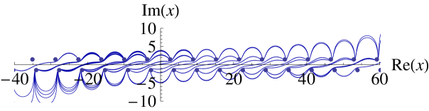
Figure 1: A typical trajectory of a particle governed by the cosine potential. Here, $E=1.99+i$ and $x(0)=0.1i$. This particle does not exhibit periodic or quasiperiodic behavior; it just hops at random from site to site.

To gain a heuristic understanding of the behavior of trajectories with energies satisfying (9), we use a numerical approach. We find that when $s$ is odd, the trajectories are periodic (see Figs. 2 and 3). When $s$ is even, the trajectories satisfy $x(t+T)=x(t)\pm 2\pi$ (see Figs. 4 and 5). Thus, our numerical work shows that we must take great care in interpreting the inversion of the integral in (6).

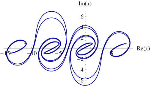
Figure 2: Periodic trajectory of a particle of complex energy $E=-0.30905+i$. The particle starts at $x=0.2i$ and the value of the ratio $R(E)$ is $17/20$. Because the $R(E)$ is reduced to lowest terms and the integer $17$ in the numerator is odd, the trajectory $x(t)$ satisfies the phenomenological rule that $x(t+T)=x(t)$. If the values of the numerator and denominator are increased, the trajectories get progressively more complicated.

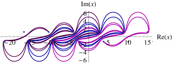
Figure 3: Periodic trajectories of a particle of energy $E=1.43696+i$. Again, the trajectories are periodic because the numerator in the ratio $R(E)=5/12$ is odd. Three trajectories are shown, one starting at $-2\pi+0.2i$, a second starting at $0+0.2i$, and a third starting at $2\pi+0.2i$. (These trajectories are purple, blue, and magenta in the electronic version.) Note that if a trajectory is translated by $2\pi$ to the left or to the right, it still does not intersect another trajectory.

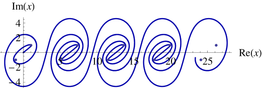
Figure 4: Quasi-periodic trajectory of a particle with energy $E=-0.779757+i$ starting at $x=0$. For this particle the numerator $8$ in the ratio $R(E)=8/9$ is even, so the trajectory $x(t)$ is quasiperiodic; that is, it satisfies $x(t+T)=2\pi+x(t)$. The dots represent the turning points, which satisfy $V(x)=E$.

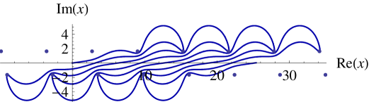
Figure 5: Quasi-periodic trajectory $x(t)$ of a particle of energy $E=2.42891+i$ starting at $x=0$. As in Fig. 4, the even numerator in the ratio $R(E)=2/9$ indicates that the trajectory is quasiperiodic.

The classical eigenenergies form a special subset of complex energies (of all possible complex energies) and the behavior of the trajectories of particles having these energies is independent of the initial position of the particle at $t=0$. Had we not determined the motion of the particle analytically, it would have been quite difficult to find energies such that the trajectory obeys $x(t+T)-x(t)\in\{0,\pm 2\pi\}$.

Let us first suppose that $E$ is real. In this case the trajectory is periodic and it is confined to one well if $E<1$. Even if $E<-1$, where the energy of the particle lies below the bottom of the potential well, the particle loops around a pair of turning points (see r6 ). If $E>1$, then the particle moves with an average velocity along the positive- or negative-real $x$ axis. If $E=1$, the particle approaches a turning point as $t\to\infty$.

If we solve (9) for complex $E$ for different rational numbers $s/r$, we can plot the energies in the complex plane (see Fig. 6). Since $R(E)$ is a continuous function almost everywhere, the relationship between the set of special energies and the set of all complex energies is the same as the relationship between the set of rational numbers and the set of all real numbers; that is, the set of all special energies is dense in the complex plane, but it is also of measure zero in the complex plane. Observe that there is a singular point in the complex plane at $E=1$. It is not surprising that $E=1$ corresponds to a singular point because this corresponds to a particle being at the top of the potential wells.

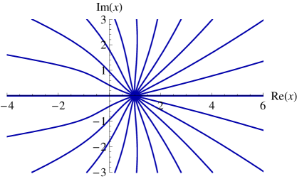
Figure 6: A plot of the complex $E$ plane. From right to left, the curves correspond to energies with $R(E)=1/10,\,2/10,\,\ldots,\,9/10,\,1$ in the upper-half complex plane. In the lower half complex plane, $R(E)$ has the opposite sign. Numerical work shows that the ratio $R(E)$ falls between $-1$ and $1$. Because the potential is real, if $x(t)$ is a solution with energy $E$, the complex conjugate of $x(t)$ with complex-conjugate energy $E^{*}$ is also a solution. Thus, there is a symmetrical plot of eigenenergies in the lower-half complex plane.

IV Determining the Periodic Motion from the Ratio $s/r$

In Ref. r7 the ratio $s/r$ was used to predict the shape of a complex trajectory. Thus, it is natural to ask the same question here: Using just the ratio $s/r$, what can we say about the behavior of the trajectories? For example, the particle might move right two wells, left one well, right two wells, left one well, and so on. We will show that the pattern of wells the particle visits is an easily calculated function of the energy.

We consider a specific example in order to demonstrate how to determine the pattern of motion from the ratio. In Fig. 7 we record the motion of a particle with ratio $9/13$ and $E=0.999931+0.0001i$ as follows: We write $+$ if the particle continues moving in the same direction at a red dot and write $-$ if the particle changes directions at a red dot. (We begin by assuming that ${\rm Im}\,E$ is small because the pattern of hopping from well to well is easiest to understand.) Then the pattern is

$$--+--+--+---+--+--+--+---+--+--+--+---$$ (10)

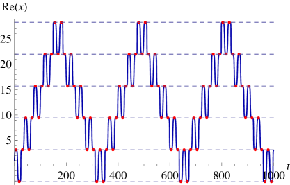
Figure 7: Plot of ${\rm Re}\,x$ as a function of time for $E=0.999931+0.0001i$ for the ratio $9/13$ and the initial position $x(0)=1+i$. The dots (red in the electronic version) indicate when the velocity of the particle is zero in the ${\rm Re}\,x$ direction. The dashed lines correspond to ${\rm Re}\,x=-\pi,\,\pi,\,3\pi$, or the $x$ values that correspond to the tops of the potential $V(x)=-\cos(x)$. The region bounded by the lowest pair of dashed lines corresponds to the particle being in the well centered at $x=0$ with boundaries at $x=\pm\pi$. There is a definite pattern; at each red point the particle decides whether to reverse direction and stay in the well in which it started or to move to an adjacent well.

Note that there is a pair of minuses, a plus, a pair of minuses, a $+$, a pair of minuses, a $+$, three minuses, a plus, and then the pattern repeats. Our goal is to predict this pattern of plus and minus signs using just the ratio $9/13$.

We define the function

$$f_{\alpha}(n)=\lfloor(n+1)\alpha\rfloor-\lfloor n\alpha\rfloor,$$ (11)

where $\alpha=9/13$. Then consider the sequence $\{f_{\alpha}(n)\}_{n=1}^{\infty}$. The first few terms are as follows:

$$1,1,0,1,1,0,1,1,0,1,1,1,0,1,1,0,1,1,0,1,1,0,1,1,1,0,1,1,0,1,1,0,1,1,0,1,1,1,0,1.$$ (12)

If we associate $f=1$ with $-$ and $f=0$ with $+$ when we comparing (10) and (12), we find that these two sequences match exactly. Numerical work shows that this method of determining the order in which a particle with a particular energy visits the wells works for all energies (see Appendix).

V Long-Time Behavior

Having established that we can use the ratio $s/r$ to predict the pattern of particles hopping from well to well, we can then predict the long-time behavior of the classical particle. Whenever a particle closely approaches a boundary between wells, it can either conduct into the next well or it can turn around and stay in the same well. Therefore, we introduce the following measure: Let $g_{n}(E)$ be the net number of wells to which the particle has moved after $n$ close approaches to boundaries between wells divided by n for a particular energy $E$. For example, consider a case in which a particle conducts twice, turns around twice, and the pattern repeats. If the particle is initially in the well $[-\pi,\pi]$ and moving in the $+Re(x)$ direction, the state of the particle, from start to finish, would progress as $([-\pi,\pi],+),\,([\pi,3\pi],+),\,([3\pi,5\pi],+),\,([3\pi,5\pi],-),\,([3\pi,5\pi],+)$, and so on. This will result in a net displacement of 2 wells in a total of 4 close approaches to the boundaries between wells. So $g_{n}(E)$ would be $2/4=1/2$ in this example.

If we examine $g_{n}(E)$ for progressively longer times (or equivalently, for more and more times where the particle remains in the same well or conducts into an adjacent well), the graph of $g_{n}(E)$ becomes more complicated. This procedure produces a fractal-like graph where $g_{\infty}(E)=0$ except when the energy $E$ is such that $R(E)$ is a rational number with an even numerator.

To produce the following graphs we use $E$ to calculate the ratio $R(E)$ from (9). The details of extending from rational to irrational ratios are discussed in the Appendix. Then from $f$ we determine whether or not the particle is going to change direction. Finally, we use this information to calculate $g$, our measure of the motion of the particle.

V.1 The Measure $g_{n}(E)$ Compared with Previous Research

Using $R(E)$ to study the motion of the particles involves detailed numerical observations, so it is helpful to show that the method described in Sec. IV is consistent with previous research on the potential $V(x)=-\cos x$. Consider Fig. 8 (taken from Ref. r6 ). This plot indicates that there are bands of energies that give rise to delocalized behavior.

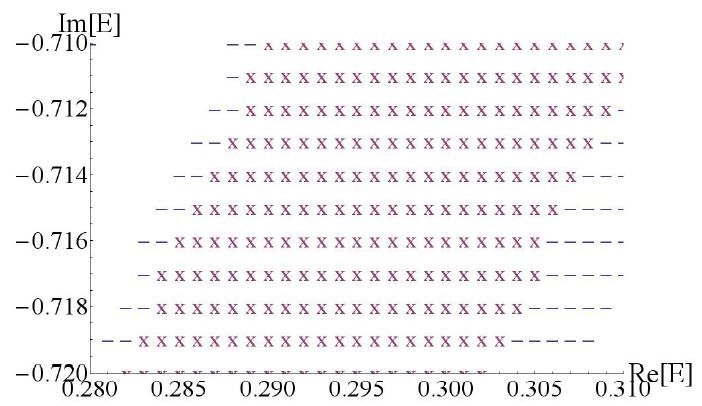
Figure 8: This plot shows the behavior of a particle under the influence of the periodic potential as a function of a complex energy. The X’s refer to the particle conducting, or being delocalized. The -’s refer to the particle staying localized. On the basis of this figure one might conclude that there are sharply defined boundaries between the energies that give rise to conducting behavior and the energies that give rise to localized behavior. However, as explained in this paper, this conclusion is not correct; the apparent sharpness of the band is an artifact of observing the particle for a fixed amount of time.

If our method is to agree with the research reported in r6 , then the energies that have X’s in Fig. 8 will have a nonzero value of $g_{n}(E)$. For energies that have minuses in Fig. 8, $g_{n}(E)$ should be near zero. Indeed, Fig. 9 verifies the correspondence between the two methods. We get an almost identical band of energies such that $g_{100}(E)=0.2$ where there were plus signs in Fig. 8 r11 . In the regions of minuses of Fig. 8, $g_{100}(E)$ is near zero.

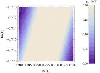
Figure 9: Average displacement of the complex classical particle after 100 close approaches to the boundaries between wells. The horizontal and vertical axes give the real and imaginary parts of the energy. The intensity of each region indicates the value of $g_{100}(E)$. The energy range is the same as in Fig. 8. The plots are in good agreement; the boundaries between the so-called conducting and localized regions match very closely.

However, as discussed earlier, the dynamics are not as simple as Fig. 8 suggests. When we examine the long-time behavior (that is, when we measure the average displacement for an even longer time), we find that the band fractures into multiple bands as shown in Fig. 10. Yet, even though the band divides into multiple bands, the center of both bands still corresponds to an average displacement of one well for every five close approaches to well boundaries.

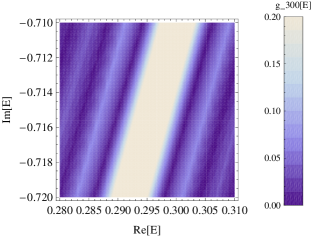
Figure 10: Same as Fig. 9 except that $n=300$ instead of $100$. Observe that the center of the band still corresponds to an average displacement of one well per five close approaches to the turning points between wells, but that the apparent band in Fig. 9 has fractured. If we look still further into the future of the particle, we see that the energy band edge is not sharp.

As we let $n$ approach infinity, the bands continue to divide and we get a fractal-like structure. In Fig. 11 we remove the unnecessary dimension of the imaginary part of the energy and just focus on a plot of $g$ as a function of ${\rm Re}\,E$ where ${\rm Im}\,E$ is fixed to be 1. This figure demonstrates how the fractal-like nature of $g_{n}(E)$ develops when $n$ becomes large.

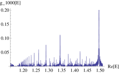
Figure 11: A plot of $g_{1000}({\rm Re}\,E+i)$ for ${\rm Re}\,E$ ranging from $1.15$ to $1.51$. Notice that there are no traces of bands with finite widths. The cascade of spikes at ${\rm Re}\,E=1.49555,\,1.34399,\,1.28908,\,\ldots$ corresponds to $R(E)=2/5,\,4/9,\,6/13,\,\ldots$, where the heights of the spikes are $1/5,\,1/9,\,1/13$, respectively. These ratios have the form $2m/(4m+1)$, where $m$ is an integer and the height of such a spike is $1/(4m+1)$. There is an accumulation point at ${\rm Re}\,E=1.16990$ where $R(E)=1/2$. Because this fraction has an odd numerator, this motion is localized. Thus, we see a transition from nonlocalized behavior (associated with an even numerator) to localized behavior (associated with an odd numerator). This image contains quasi-self-similar features: There is a cascade of spikes of decreasing height and these spikes accumulate at certain energies for sequences of energies with ratios of the form $2m/(2am+1)$ for a fixed integer $a$ and all $m$.

V.2 Energy Dependence of Long-Time Behavior

We have demonstrated numerically that if $R(E)=\alpha=p/q$ [in the sense of (9)] where $p$ and $q$ are relatively prime, then $g_{\infty}(E)=1/q$ if $p$ is even and $g_{\infty}(E)=0$ if $p$ is odd. If $\alpha$ is irrational, then $g_{\infty}=0$. We examine $g_{n}$ as $n$ goes to infinity for $E$ such that $R(E)=\alpha$ is irrational. To study $g_{n}(E)$ we approximate $\alpha$ by a suitably close rational number. Our numerical experience shows that if we examine only up to a fixed number $n$ of close approaches to boundaries between wells, we can always find such a rational number $p/q$ and corresponding energy $E^{\prime}$ that reproduces the behavior demonstrated by $\alpha$ and $E$. As we choose better rational-number approximations for $\alpha$, we note that the denominators of such approximations approach infinity. Since $g_{n}(E^{\prime})$ is either $0$ or $1/q$ with $q$ becoming arbitrarily large as we choose better rational approximations for $\alpha$, $g_{n}(E)\to 0$ as $n\to\infty$. Thus, the particle motion is localized in the sense that the average velocity is zero for all but a set of measure zero of energies.

VI Concluding Remarks

In this paper we have tried to characterize the motion of a complex classical particle in a periodic potential. We have identified interesting trajectories and have described the pattern of jumping from one well to another.

The results presented here are largely consistent with earlier work in which it was observed that in the complex domain classical and quantum mechanics exhibit many similar features. However, we have discovered new and interesting behaviors. Not surprisingly, when we look at the long-time behavior of a dynamical system, we observe fractal-like behavior. We have shown that for irrational numbers, the so-called average velocity is zero. However, this does not eliminate the possibility that the displacement grows as a function such as $\log t$ that is much smaller than $t$. It may be that the motion of the particle is chaotic for energies having an irrational ratio. That is, the particle jumps from well to well in a pattern that does not have a well-defined asymptotic behavior. However, because the particle does not coordinate its hops in a particular direction, the average displacement is much less than the number of jumps of the particle.

Appendix A Details Concerning the Pattern

A.1 Motivating the Use of $f$ to Determine the Well-Jumping Pattern

Recall the form of the solution for $x(t)$ in (7). The function ${\rm am}(z|m)$ is quasiperiodic in two directions in the complex-$z$ plane. These periods are $2K(m)$ and $2iK(1-m)$. Note that $x(t)$ has the form $2{\rm am}(At+B,m)$, where $A$ and $B$ are complex constants. So, as time evolves, $At+B$ moves through a doubly periodic domain. As a concrete example, consider a ratio of $9/13$. The choice $R(E)=9/13$ corresponds to $At+B$ going through $13$ periods of $2K(m)$ and $9$ periods of $2iK(1-m)$ in the time interval $[0,T]$. This is shown in Fig. 12.

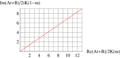
Figure 12: The axes show the real and imaginary parts of $At+B$ scaled by the periods in those two directions. If the energy is real, then $2K(m)$ is real and $2iK(1-m)$ is imaginary. When $E$ becomes complex, the periods are no longer orthogonal and the grid of rectangles shown in this figure becomes a grid of parallelograms.

Now we can interpret the meaning of the function $f_{\alpha}(n)$, as defined in (11); $n\alpha$ is the $y$ value of the red line in Fig. 12 for an $x$ value of $n$. We can see that $\lfloor(n+1)\alpha\rfloor-\lfloor n\alpha\rfloor$ is equal to one if the red line crosses a horizontal line between the vertical lines $x=n$ and $x=n+1$, and is zero otherwise. That is, if we cross a horizontal line, we have $f=1$, which corresponds to a $-$ [as in Eq. (10)], and a change of direction at a red dot (as in Fig. 7). So, crossing a horizontal line in Fig. 12 should correspond to the particle moving in the opposite direction.

We can verify this analytically. If we move up one period [that is, $z\to z+2iK(1-m)$], we expect the particle to be moving in the opposite direction. We can use the following elliptic-function identities to show that there is indeed a change in sign of $dx/dt$:

$$\frac{dx}{dt}=2\frac{d}{dt}{\rm am}(At+B|m)=2dn(At+B|m)(A),$$ (A1)

$$dn(z+2iK(1-m)|m)=-dn(z|m),$$ (A2)

where $dn(z|m)$ is a standard elliptic function. Although the details of taking the functional inverse to find the form for $x(t)$ are complicated, this calculation helps to explain why the function $f_{\alpha}(n)$ is relevant to this problem.

A.2 Numerical Justification of the use of the Pattern

Extending from small ${\rm Im}\,E$ to any ${\rm Im}\,E$: To identify the hopping pattern we have assumed that the imaginary part of the energy is small so that the boundaries of the wells are relatively well defined (as in Fig. 7). However, extensive numerical work indicates that even if we let the imaginary part of the energy be large, we still obtain the same behavior.

As the imaginary part of the energy increases, two things happen. First, the locations of the wells become less defined. However, the pattern of moving from well to well remains the same, where we define the wells by the intervals $[-\pi,\pi]$, $[\pi,3\pi]$, etc. This can be verified, for example, by plotting ${\rm Re}\,x$ as a function of $t$ for energies that have a ratio of $9/13$ with ${\rm Im}\,E=0.01,\,0.1,\,1$ (see Fig. 13).

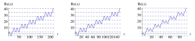
Figure 13: Plots of ${\rm Re}\,x$ as a function of time for $x(0)=0.1i$, $R(E)=4/5$, and varying ${\rm Im}\,E$. The dotted lines correspond to the maxima of $V(x)$ on the real axis. From left to right, $E=0.986436+0.01i$, $0.874181+0.1i$, $0.0627904+i$ and the time is taken out to $t=215,152,94$. Notice that as ${\rm Im}\,E$ increases, the trajectories deform and the time axis deforms. These plots demonstrate qualitatively that as ${\rm Im}\,E$ decreases, the time required to “tunnel” from one well to another increases. Nevertheless, we can see that even though the trajectories deform, the general behavior of moving from one well to another remains the same even when ${\rm Im}\,E$ is not small. Furthermore, these plots demonstrate that the function $g_{n}(E)$ is a relatively good approximation to the average velocity as a function of energy.

Second, the time between close approaches to the boundaries of the wells changes. However, this change happens slowly. Using the trajectories in Fig. 13, one can also see that the time needed to move from one well to another varies, but even for energies having small imaginary parts, this time does not approach $\infty$ like $1/{\rm Im}\,E$. For instance, for a ratio of $9/13$, and ${\rm Im}\,E=0.1$, this time is about $5$ and for ${\rm Im}\,E=10^{-5}$, this time is about 10. This is contrary to previous research that had suggested that the tunneling time is inversely proportional to the imaginary part of the energy.

Extending from $E$ with a rational ratio to $E$ with an irrational ratio: We have assumed that the energy is such that $R(E)$ is rational. However, whether or not $R(E)$ is rational is unimportant if we are tracking the particle for a fixed amount of time because the difference between the motion for energies that are close does not show up until a large time $t$. Thus, if we examine the motion of a particle where $R(E)$ is irrational up to some fixed time $t$, we can choose an energy $E^{\prime}$ such that $R(E^{\prime})$ is rational and such that the two trajectories are practically identical in the time interval $[0,t]$ for any $t$.

References

- (1) A. Nanayakkara, Czech. J. Phys. 54, 101 (2004) and J. Phys. A: Math. Gen. 37, 4321 (2004).
- (2) C. M. Bender, D. D. Holm, and D. W. Hook, J. Phys. A: Math. Theor. 40, F81 (2007).
- (3) C. M. Bender, D. D. Holm, and D. W. Hook, J. Phys. A: Math. Theor. 40, F793-F804 (2007).
- (4) C. M. Bender, D. C. Brody, and D. W. Hook, J. Phys. A: Math. Theor. 41, 352003 (2008).
- (5) C. M. Bender, D. W. Hook, and K. S. Kooner, J. Phys. A: Math. Theor. 43, 165201 (2010).
- (6) T. Arpornthip and C. M. Bender, Pramana-J. Phys. 73, 259 (2009).
- (7) A. G. Anderson, C. M. Bender, and U. I. Morone, Phys. Lett. A 375, 3399 (2011).
- (8) A. J. Brizard, Eur. J. Phys. 30, 729 (2009).
- (9) J. V. Armitage and W. F. Eberlein, Elliptic Functions, London Mathematical Society Student Texts (No. 67), (Cambridge University Press, Cambridge, 2006).
-
(10)
See http://functions.wolfram.com/EllipticFunctions/JacobiAmplitude
/introductions/JacobiPQs/05/. - (11) The density plots in Figs. 9 and 10 were generated by using Colorbarplot v0.6, which is available at http://www.walkingrandomly.com/?p=2960.