Tracking Topology Dynamicity for Link Prediction in Intermittently Connected Wireless Networks

Abstract

Through several studies, it has been highlighted that mobility patterns in mobile networks are driven by human behaviors. This effect has been particularly observed in intermittently connected networks like DTN (Delay Tolerant Networks). Given that common social intentions generate similar human behavior, it is relevant to exploit this knowledge in the network protocols design, e.g. to identify the closeness degree between two nodes. In this paper, we propose a temporal link prediction technique for DTN which quantifies the behavior similarity between each pair of nodes and makes use of it to predict future links. We attest that the tensor-based technique is effective for temporal link prediction applied to the intermittently connected networks. The validity of this method is proved when the prediction is made in a distributed way (i.e. with local information) and its performance is compared to well-known link prediction metrics proposed in the literature.

I Introduction

In recent years extensive research has addressed challenges and problems raised in mobile, sparse and intermittently connected networks (i.e. DTN). In this case, forwarding packets greatly depends on the occurrence of contacts. Since the existence of links is crucial to deliver data from a source to a destination, the contacts and their properties emerge as a key issue in designing efficient communication protocols [1]. Obviously, the occurrence of links is determined by the behavior of the nodes in the network [2]. It has been widely shown in [3, 4] that human mobility is directed by social intentions and reflects spatio-temporal regularity. A node can follow other nodes to a specific location (spatial level) and may bring out a behavior which may be regulated by a schedule (temporal level). The social intentions that govern the behavior of mobile users have also been observed through statistical analyses in [2, 5] by showing that the distribution of inter-contact times follow a truncated power law.

With the intention of improving the performance of intermittently connected wireless network protocols, it is paramount to track and understand the behavior of the nodes. We aim to propose an approach that analyzes the network statistics, quantifies the social relationship between each pair of nodes and exploits this measure as a score which indicates if a link would occur in the immediate future.

In this paper, we adapt a tensor-based link prediction algorithm successfully designed for data-mining [6, 7]. Our proposal records the network structure for $T$ time periods and predicts links occurrences for the $(T+1)^{th}$ period. This link prediction technique is designed through two steps. First, tracking time-dependent network snapshots in adjacency matrices which form a tensor. Second, applying of the Katz measure [8] inspired from sociometry. To the best of our knowledge, this work is the first to perform the prediction technique in a distributed way. The assessment of its efficiency can be beneficial for the improvement or the design of communication protocols in mobile, sparse and intermittently connected networks.

The paper is organized as follows: Section 2 presents the related work that highlights the growing interest to the social analysis and justifies the recourse to the tensors and to the Katz measure to perform predictions. In Section 3, we describe the two main steps that characterize our proposal. Section 4 details simulation scenarios used to evaluate the tensor-based prediction approach, analyzes the obtained results and assesses its efficiency. Finally, we conclude the paper in Section 5.

II Related Work

Social Network Analysis (SNA) [9, 10] and ad-hoc networking have provided new perspectives for the design of network protocols [11, 12, 13]. These protocols aim to exploit the social aspects and relationship features between the nodes. Studies conducted in the field of SNA have mainly focused on two kinds of concepts: the most well-known centrality metrics suggested in [9, 14, 15, 16] and the community detection mechanisms proposed in [17, 18, 19, 9]. From this perspective, several works have tried to develop synthetic models that aim to reproduce realistic moving patterns [3, 20]. Nonetheless, the study done in [1] has underlined the fact that synthetic models cannot faithfully reproduce human behavior because these synthetic models are only location-driven and they do not track social intentions explicitly.

In their survey, Katsaros et al. [10] have underlined the limits of these protocols when the network topology is time-varying. The main drawback comes down to their inability to model topology changes as they are based on graph theory tools. To overcome this limit, tensor-based approaches have been used in some works to build statistics on the behavior of nodes in wireless networks over time as in [21]. Thakur et al. [4] have also developed a model using a collapsed tensor that tracks user’s location preferences (characterized by probabilities) with a considered time granularity (week days for example) in order to follow the emergence of “behavior-aware" delay tolerant networks closely.

As previously mentioned, tracking the social ties between network entities enables us to understand how the network is structured. Such tracking has led to the design of techniques for link prediction. Link prediction in social networks has been addressed in data mining applications as in [6, 7]. Concerning link prediction in community-based communication networks, [22] has highlighted salient measures that allow link occurrence between network users to be predicted. These metrics determine if a link occurrence is likely by quantifying the degree of proximity of two nodes (Katz measure [8], the number of common neighbors, Adamic-Adar measure [23], Jaccard’s coefficient [24, 25], …) or by computing the similarity of their mobility patterns (spatial cosine similarity, co-location rate, …).

In this paper, we propose a link prediction technique that tracks the temporal network topology evolution in a tensor and computes a metric in order to characterize the social-based behavior similarity of each pair of nodes. Some approaches have addressed the same problem in data-mining in order to perform link prediction. Acar et al. [6] and Dunlavy et al. [7] have provided detailed methods based on matrix and tensor factorizations for link prediction in social networks such as the DBLP data set [26]. These methods have been successfully applied to predict a collaboration between two authors by recording the structure of relationships over a tracking period. Moreover, they have highlighted the use of the Katz measure [8], which can be seen as a behavior similarity metric, by assigning a link prediction score for each pair of nodes. The efficiency of the Katz measure in link prediction has been also demonstrated in [6, 7, 22, 28].

III Description of the Tensor Based Prediction Method

It has been highlighted that a human mobility pattern shows a high degree of temporal and spatial regularity, and each individual is characterized by a time-dependent mobility pattern and a trend to return to preferred locations [2, 3, 4]. In this paper, we propose an approach that aims to exploit similar behavior of nodes in order to predict link occurrence referring to the social closeness.

To quantify the social closeness between each pair of nodes in the network, we use the Katz measure [8] inspired by sociometry. This measure aims at quantifying the social distance between people inside a social network. We also need to use a structure that records link occurrence between each pair of nodes over a certain period of time in order to perform the similarity measure computation. The records represent the network behavior statistics in time and space. To this end, a third-order tensor is considered. A tensor $\boldsymbol{\mathcal{Z}}$ consists of a set of slices and each slice corresponds to an adjacency matrix of the network tracked over a given period of time $p$. After the tracking phase, we reduce the tensor into a matrix (or collapsed tensor) which expresses the weight of each link according to its lifetime and its recentness. A high weight value in this matrix denotes a link whose corresponding nodes share a high degree of closeness. We apply the Katz measure to the collapsed tensor to compute a matrix of scores $\mathbf{S}$ that not only considers direct links but also indirect links (multi-hop connections). The matrix of scores expresses the degree of similarity of each pair of nodes according to the spatial and the temporal levels. The higher the score is, the better the similarity pattern gets. Therefore, two nodes that have a high similarity score are more likely to have a common link in the future.

III-A Notation

Scalars are denoted by lowercase letters, e.g., $a$. Vectors are denoted by boldface lowercase letters, e.g., $\bf{a}$. Matrices are denoted by boldface capital letters, e.g., $\mathbf{A}$. The $r^{th}$ column of a matrix $\mathbf{A}$ is denoted by $\bf{a_{r}}$. Higher-order tensors are denoted by bold Euler script letters, e.g., $\boldsymbol{\mathcal{T}}$. The $n^{th}$ frontal slice of a tensor $\boldsymbol{\mathcal{T}}$ is denoted $\mathbf{T_{n}}$. The $i^{th}$ entry of a vector $\bf{a}$ is denoted by $\bf{a}(i)$, element $(i,j)$ of a matrix $\mathbf{A}$ is denoted by $\mathbf{A}(i,j)$, and element $(i,j,k)$ of a third-order tensor $\boldsymbol{\mathcal{T}}$ is denoted by $\mathbf{T_{i}}(j,k)$.

III-B Matrix of Scores Computation

The computation of the similarity scores is modeled through two distinct steps. First, we store the inter-contact between nodes in a tensor $\boldsymbol{\mathcal{Z}}$ and reduce it to a matrix $\mathbf{X}$ called the collapsed tensor. In a second step, we compute the matrix of similarity scores $\mathbf{S}$ relying on the matrix $\mathbf{X}$ (cf. Fig. 1).

We consider that the data is collected into the tensor $\boldsymbol{\mathcal{Z}}$. The slice $\mathbf{Z_{p}}(i,j)$ describes the status of a link between a node $i$ and a node $j$ during a time period $[(p-1)\cdot t,p\cdot t[$ ($p$>0) where $\mathbf{Z}_{p}(i,j)$ is 1 if the link exists during this period and 0 otherwise. The tensor is formed by a succession of adjacency matrices $\mathbf{Z_{1}}$ to $\mathbf{Z_{T}}$ where the subscript letters designate the observed period. To collapse the data into one matrix as done in [6, 7], we choose to compute the collapsed weighted tensor (which is the most efficient way to collapse the data as shown in [6] and [7]). The links structure is considered over time and the more recent the adjacency matrix is, the more weighted the structure gets. The collapsed weighted tensor is computed as following:

$$\mathbf{X}(i,j)=\sum_{p=1}^{T}(1-\theta)^{T-t}\ \mathbf{Z_{p}}(i,j)$$ (1)

where the matrix $\mathbf{X}$ is the collapsed weighted tensor of $\boldsymbol{\mathcal{Z}}$, and $\theta$ is a parameter used to adjust the weight of recentness and is between 0 and 1.

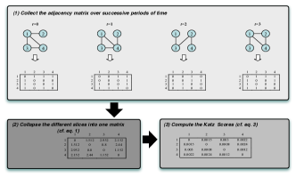
Figure 1: Example of the matrix $\mathbf{S}$ computation

As Katz measure quantifies the network proximity between two nodes and given that there are “social relationships" between nodes in networks with intermittent connections, it is challenging to exploit this measure and to apply it on the collected data. Therefore, the Katz score of a link between a node $i$ and a node $j$ as given by [8]:

$$\mathbf{S}(i,j)=\sum_{\ell=1}^{+\infty}\beta^{\ell}P_{\left\langle\ell\right\rangle}(i,j)$$ (2)

where $\beta$ is a user defined parameter strictly superior to zero, $\beta^{\ell}$ is the weight of a $\ell$ hops path length and $P_{\left\langle\ell\right\rangle}(i,j)$ represents the number of paths of length $\ell$ that join the node $i$ to the node $j$.

It is clear that the longer the path is, the lower the weight gets. There is also another formulation to compute Katz scores by means of collapsed weighted tensor as detailed previously. We quantify the proximity between nodes relying on the paths that separate a pair of nodes and the weights of the links that form these paths. Then, the score matrix $\mathbf{S}$ can be rewritten as:

$$\mathbf{S}=\sum_{\ell=1}^{+\infty}\beta^{\ell}\cdot\mathbf{X}^{\ell}=(\mathbf{I}-\beta\cdot\mathbf{X})^{-1}-\mathbf{I}$$ (3)

Where $\mathbf{I}$ is the identity matrix and $\mathbf{X}$ is the collapsed weighted tensor obtained.

We depict as previously mentioned in Fig. 1 an example which details the two major steps described before. We take into consideration a network consisting of 4 nodes and having a dynamic topology over 4 time periods and we highlight how similarity scores are obtained. The parameters $\theta$ and $\beta$ are respectively set to 0.2 and 0.001 for the example and later for the simulations. We have looked after the values to choose for these two parameters through several simulations and we have found that such a setting make possible the convergence of the Katz measure as explained in [29]. In this example, we assume that all nodes have the full knowledge of the network structure.

IV Performance Evaluation and Simulation Results

To evaluate how efficient is the tensor-based link prediction in intermittently connected wireless networks, we consider two real traces. In the following, we firstly present the traces used for the link prediction evaluation. Then, we expose the corresponding results, analyze the effectiveness of the prediction method and compare its performance to those of well-known link prediction metrics proposed in the literature.

IV-A Simulation Traces

We consider two real traces to evaluate the link prediction approach. We exploit them to construct the tensor by generating adjacency matrices for several tracking periods. For each case, we track the required statistics about network topology within $T$ periods. We also consider the adjacency matrix corresponding to the period $T$+1 as a benchmark to evaluate Katz scores matrix. We detail, in the following, the used traces.

• First Trace: Dartmouth Campus trace: we choose the trace of 01/05/06 [30] and construct the tensor slices relying on SYSLOG traces between 8 a.m. and 3 p.m. (7 hours). The number of nodes is 1018 and the number of locations (i.e. access points) is 128.

• Second Trace: MIT Campus trace: we focus on the trace of 07/23/02 [31] and consider also the events between 8 a.m. and 3 p.m. to build up the tensor. The number of nodes is 646 and the number of locations (i.e. access points) is 174.

For each scenario, we generate adjacency matrices corresponding to a different tracking periods $t$: 5, 10, 30 and 60 minutes. To record the network statistics over 7 hours, the tensor has respectively a number of slices $T$ equal to 84, 42, 14 and 7 slices (for the case where $t$=5 minutes, it is necessary to have 84 periods to cover 7 hours). We take into account both centralized and distributed cases for the computation of scores.

• The Centralized Computation: the centralized way assumes that there is a central entity which has full knowledge of the network structure at each period and applies Katz measure to the global adjacency matrices.

• The Distributed Computation: each node has a limited knowledge of the network structure. We assume that a node is aware of its two-hop neighborhood. Hence, computation of Katz measures is performed on a local-information-basis.

IV-B Performance Analysis

As described in the previous section, we apply the link prediction method to the traces with considering different tensor slice periods in both centralized and distributed cases. In order to assess the efficiency of this method, we consider several link prediction scenarios (according to the trace, the tensor slice period and the scores computation way) and we use different evaluation techniques. We detail in the following the results obtained for the evaluation and analyze the link prediction efficiency. Then, we compare the performance of the proposed framework to those of major link prediction metrics in order to justify the use of the Katz measure.

IV-B1 Evaluation of the link prediction technique

To evaluate the efficiency of our proposal, we plot the ROC curves (Receiver Operating Characteristic curves) [32]. In Fig. 2, we depict the ROC curves obtained after performing prediction on the Dartmouth Campus trace and for different tensor slice times. Also, adapted metrics are used in order to weigh the performance of the proposed link prediction technique. To this end, we compute the Area Under the ROC Curve metric (AUC metric) [32] which could be considered as a good performance indicator in our case. The AUC metric of each scenario is determined from the corresponding ROC curve. Moreover, we consider the top scores ratio metric at $T$+1. To determine this metric, we compute the accurate number of links identified through the link prediction technique. We list, for each considered time period, the number of existing links at period $T$+1, which we call $L$. Then, we extract the links having the $L$ highest scores and determine the number of existing links in both sets. The evaluation metrics are computed for all traces with different tensor slice periods in both distributed and centralized scenarios. The results corresponding to all links prediction are listed in Table I (Dartmouth Campus trace)and Table II (MIT Campus trace).

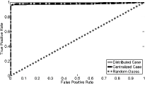
(a) 5 minutes tensor slice period

(b) 10 minutes tensor slice period

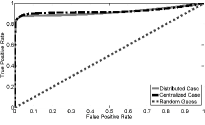
(c) 30 minutes tensor slice period

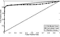
(d) 60 minutes tensor slice period

Figure 2: ROC Curves for different prediction cases applied on Dartmouth Campus trace

TABLE I: Evaluation metrics for the prediction of all links applied on Dartmouth Campus trace

	AUC	Top Scores Ratio at $T$+1
Distributed Case and $t$=5 mins	0.9932	93.70%
Centralized Case and $t$=5 mins	0.9905	93.61%
Distributed Case and $t$=10 mins	0.9915	90.26%
Centralized Case and $t$=10 mins	0.9883	90.19%
Distributed Case and $t$=30 mins	0.9813	82.31%
Centralized Case and $t$=30 mins	0.9764	82.56%
Distributed Case and $t$=60 mins	0.9687	76.10%
Centralized Case and $t$=60 mins	0.9636	75.94%

TABLE II: Evaluation metrics for the prediction of all links applied on MIT Campus trace

	AUC	Top Scores Ratio at $T$+1
Distributed Case and $t$=5 mins	0.9907	91.48%
Centralized Case and $t$=5 mins	0.9929	91.48%
Distributed Case and $t$=10 mins	0.9797	85.18%
Centralized Case and $t$=10 mins	0.9809	85.14%
Distributed Case and $t$=30 mins	0.9589	73.31%
Centralized Case and $t$=30 mins	0.9578	73.76%
Distributed Case and $t$=60 mins	0.9328	64.54%
Centralized Case and $t$=60 mins	0.9325	64.54%

TABLE III: Table of confusion of a binary prediction technique

	Positive	Negative
Positive	True Positive ($TP$)	False Positive ($FP$)
Negative	False Negative ($FN$)	True Negative ($TN$)

We first note that, in Fig. 2 and for all scenarios, the prediction of all links is quite efficient, compared to the random guess (the curve’s bends are at the upper left corner). We obtain similar ROC curves with the MIT Campus traces (we do not present them due to space limitations). Moreover, we remark, based on the high values of AUC metric (over than 0.9) and top scores ratio obtained at $T$+1, that the prediction method is efficient in predicting future links (for the period $T$+1). We also note that prediction is better when the tensor slice periods are shorter. This observation is obvious for two reasons. On the one hand, with a low tensor slice time, the probability of tracking a short and occasional contact between two nodes is not likely. On the other hand, recording four hours of statistics requires 84 adjacency matrices of 5-minute periods instead of 7 matrices for 60-minute periods case. Thus, tracking a short contact between two nodes has less influence when the tensor slices are more numerous.

Regarding the comparison between the two ways of computing the Katz scores, we observe that the centralized and distributed matrix of scores computation achieve similar performances. In fact, the similarity is higher when the paths considered between a pair of nodes are short. Thereby, paths that have more than two hops have weaker scores and so are less weighted compared to shorter ones. The distributed case assumes that each node knows its neighbors at most at two hops. That is why distributed scores computation presents performances which are so similar to the centralized ones.

IV-B2 Prediction Performance Comparison between the Tensor-Based Technique and Well-Known Link Prediction Metrics

We aim through this subsection to compare our proposal to another similar approaches (we use the distributed design of our framework to compute the Katz scores). To propose a comprehensive comparison, we also propose to evaluate the prediction efficiency of well-known prediction metrics presented in the literature. On the one hand, we consider behavioral-based link prediction metrics as the similarity metric of Thakur et al. [4] and two metrics expressing mobile homophily proposed by Wang et al. in [22]: the spatial cosine similarity and the co-location rate. On the other hand, we take two link prediction metrics based on measuring the degree of proximity as the Katz measure: they are the Adamic-Adar measure [23] and the Jaccard’s coefficient [24, 25].

To assess the efficiency of each link prediction metric, we consider these evaluation measures:

• Top Scores Ratio in the period $T$+1 (TSR): to determine this metric, we compute the percentage of occurring links identified through the link prediction technique. We list the number of existing links (at period $T$+1 or during the periods coming after the period $T$) which we call $L$. Then, we extract the pair of nodes having the $L$ highest scores and determine the percentage of links involved in both sets. existing links in both sets.

• Accuracy (ACC): this measure is defined in [32] as the ratio of correct prediction (true positive and true negative predictions) over all predictions (true positive, true negative, false positive and false negative predictions). In other words, it is computed by the ratio $\frac{TP+TN}{TP+FP+TN+FN}$ (see Table III). We identify for each scenario the maximum value of the accuracy which indicates the degree of precision that can reach each prediction metric.

• Precision or Positive Predictive Value (PPV): it represents to the proportion of links with positive prediction (occurring in the future) which are correctly identified [32]. Based on Table III, the precision is equal to $\frac{TP}{TP+FP}$. This value is determined according to the deduced accuracy value.

• Recall or True Positive Rate (TPR): it quantifies the ratio of correctly identified links over the occurring links in the future [32]. Referring to Table III, the recall is defined by the expression $\frac{TP}{TP+FN}$. This value is also computed according to the retained accuracy value.

• F-measure or balanced F1 score: the F-measure [33] is the harmonic mean of precision and recall. The F-measure is expressed by $2.\frac{precision.recall}{precision+recall}$. The higher the F-measure is, the better the tradeoff of precision and recall gets and the more efficient the prediction metric is.

The evaluation metrics are computed for all traces with different tracking periods lengths (5, 10, 30 and 60 minutes). For each trace, we track the network topology from 8 a.m. to 4 p.m. We divide, as previously, the historical into $T$ periods and we focus on predicting the links occurring in the period $T$+1. Regarding the Dartmouth Campus trace, the results are reported in Table IV. For the MIT Campus trace, the prediction results are listed in Table V.

TABLE IV: Evaluation metrics for the prediction applied on the Dartmouth Campus trace

Period length	Prediction Score	TSR in $T$+1	Accuracy	Precision (PPV)	Recall (TPR)	F-measure
5 mins ($T$=96)	Thakur’s Metric	41.39%	99.11%	36.40%	11.57%	0.1756
	Spatial Cosine Sim.	66.01%	99.45%	67.44%	63.75%	0.6554
	Co-Location Rate	68.96%	99.50%	73.98%	60.71%	0.6669
	Adamic-Adar Meas.	83.81%	99.74%	82.58%	85.57%	0.8405
	Jaccard’s Coeff.	82.54%	99.72%	81.27%	85.08%	0.8313
	Katz Measure	90.88%	99.86%	90.59%	91.87%	0.9123
10 mins ($T$=48)	Thakur’s Metric	43.29%	99.10%	37.31%	11.15%	0.1717
	Spatial Cosine Sim.	66.71%	99.45%	68.52%	62.99%	0.6564
	Co-Location Rate	68.78%	99.49%	71.50%	65.63%	0.6844
	Adamic-Adar Meas.	81.01%	99.68%	78.87%	84.00%	0.8135
	Jaccard’s Coeff.	79.75%	99.66%	78.04%	82.83%	0.8036
	Katz Measure	86.39%	99.78%	89.75%	82.94%	0.8621
30 mins ($T$=16)	Thakur’s Metric	45.18%	99.06%	39.08%	10.83%	0.1696
	Spatial Cosine Sim.	67.35%	99.42%	67.60%	67.00%	0.6730
	Co-Location Rate	67.78%	99.45%	72.47%	61.33%	0.6644
	Adamic-Adar Meas.	71.82%	99.50%	71.25%	73.86%	0.7253
	Jaccard’s Coeff.	71.34%	99.50%	72.63%	69.65%	0.7111
	Katz Measure	79.83%	99.64%	80.09%	79.48%	0.7978
60 mins ($T$=8)	Thakur’s Metric	46.39%	99.04%	41.39%	10.61%	0.1689
	Spatial Cosine Sim.	67.55%	99.40%	68.51%	65.70%	0.6708
	Co-Location Rate	68.11%	99.42%	72.21%	60.31%	0.6573
	Adamic-Adar Meas.	65.98%	99.38%	69.73%	57.42%	0.6298
	Jaccard’s Coeff.	67.00%	99.47%	68.31%	64.53%	0.6637
	Katz Measure	74.09%	99.53%	75.33%	72.84%	0.7406

TABLE V: Evaluation metrics for the prediction applied on the MIT Campus trace

Period length	Prediction Score	TSR in $T$+1	Accuracy	Precision (PPV)	Recall (TPR)	F-measure
5 mins ($T$=96)	Thakur’s Metric	58.22%	99.29%	65.58%	44.96%	0.5335
	Spatial Cosine Sim.	60.87%	99.34%	72.56%	44.17%	0.5491
	Co-Location Rate	69.35%	99.49%	77.79%	60.71%	0.6820
	Adamic-Adar Meas.	84.20%	99.72%	84.22%	84.36%	0.8429
	Jaccard’s Coeff.	82.18%	99.68%	83.11%	81.12%	0.8210
	Katz Measure	90.14%	99.86%	95.29%	89.02%	0.9205
10 mins ($T$=48)	Thakur’s Metric	57.70%	99.27%	65.25%	44.58%	0.5569
	Spatial Cosine Sim.	60.50%	99.32%	72.56%	43.18%	0.5414
	Co-Location Rate	68.74%	99.46%	76.50%	60.08%	0.6730
	Adamic-Adar Meas.	80.04%	99.63%	79.31%	80.87%	0.8008
	Jaccard’s Coeff.	77.97%	99.59%	80.53%	73.77%	0.7700
	Katz Measure	86.83%	99.78%	86.62%	87.25%	0.8693
30 mins ($T$=16)	Thakur’s Metric	56.73%	99.20%	62.87%	46.14%	0.5322
	Spatial Cosine Sim.	59.35%	99.26%	72.65%	40.51%	0.5202
	Co-Location Rate	65.03%	99.39%	80.75%	49.93%	0.6171
	Adamic-Adar Meas.	67.07%	99.35%	67.77%	64.55%	0.6572
	Jaccard’s Coeff.	66.34%	99.39%	78.56%	51.97%	0.6214
	Katz Measure	72.85%	99.47%	88.30%	53.86%	0.7279
60 mins ($T$=8)	Thakur’s Metric	55.70%	99.08%	63.51%	41.85%	0.5045
	Spatial Cosine Sim.	57.57%	99.14%	72.82%	37.22%	0.4926
	Co-Location Rate	61.71%	99.24%	77.89%	45.10%	0.5712
	Adamic-Adar Meas.	59.13%	99.14%	57.52%	65.48%	0.6124
	Jaccard’s Coeff.	58.95%	99.22%	71.27%	45.73%	0.5571
	Katz Measure	61.00%	99.28%	74.90%	50.09%	0.6003

The results obtained enable us to attest that the use of the Katz measure has been one of the best choices to perform prediction through the tensor-based technique. Using this metric achieves better performance than those of the other link prediction metrics proposed in the literature. Hence, the Katz measure is the best metric that we can use to perform link prediction.

The prediction made through the Katz measure achieves better performance than those of mobility homophily metrics and Thakur et al.’s similarity. Indeed, our framework quantifies the similarity of nodes based on their encounters and geographical closeness. In other words, the proposed prediction method cares about contacts (or closenesses) at (around) the same location and at the same time. Meanwhile, the mobility homophily metrics and Thakur et al.’s similarity are defined as an association metric. Hence, they measure the degree of similarity of behaviors of two mobile nodes without necessarily seeking if they are in the same location at the same time. Regarding the comparison with the other network proximity metrics, the Katz measure quantifies better the behavior similarity of two nodes as it takes into consideration only the paths that separate them. Meanwhile, the Adamic-Adar metric and the Jaccard’s coefficient are dependent respectively on the degree of common neighbors between two nodes and the size of the intersection of the neighbors of two nodes. These latter metrics express similarity based on common neighbors of two nodes but don’t seek if a link is occurring between them. This criterion highly influences the value of Katz measure and make it more precise.

V Conclusion

Human mobility patterns are mostly driven by social intentions and correlations appear in the behavior of people forming the network. These similarities highly govern the mobility of people and then directly influence the structure of the network. The knowledge about the behavior of nodes greatly helps in improving the design of communication protocols. Intuitively, two nodes that follow the same social intentions over time promote the occurrence of a link in the immediate future.

In this paper, we presented a link prediction technique inspired by data mining and exploit it in the context of human-centered wireless networks. Through the link prediction evaluation, we have obtained relevant results that attest the efficiency of our contribution and agree with some findings referred in the literature.

Good link prediction offers the possibility to further improve opportunistic packet forwarding strategies by making better decisions in order to enhance the delivery rate or limiting latency. Therefore, it will be relevant to supply some routing protocols with prediction information and to assess the contribution of our approach in enhancing the performance of the network especially as we propose an efficient distributed version of the prediction method. The proposed technique also motivates us to inquire into future enhancements as a more precise tracking of the behavior of nodes and a more efficient similarity computation.

References

- [1] T. Hossmann, T. Spyropoulos, and F. Legendre, “Social network analysis of human mobility and implications for dtn performance analysis and mobility modeling,” Computer Engineering and Networks Laboratory ETH Zurich, Tech. Rep. 323, July 2010.
- [2] A. Chaintreau, P. Hui, J. Crowcroft, C. Diot, R. Gass, and J. Scott, “Impact of human mobility on opportunistic forwarding algorithms,” IEEE Trans. on Mobile Computing, vol. 6, no. 6, pp. 606–620, June 2007.
- [3] W.-J. Hsu, T. Spyropoulos, K. Psounis, and A. Helmy, “Modeling Spatial and Temporal Dependencies of User Mobility in Wireless Mobile Networks,” IEEE/ACM Trans. on Networking, vol. 17, no. 5, pp. 1564–1577, October 2009.
- [4] G. S. Thakur, A. Helmy, and W.-J. Hsu, “Similarity analysis and modeling in mobile societies: the missing link,” in Proc. of the 5th ACM workshop on Challenged networks (CHANTS ’10), 2010, pp. 13–20.
- [5] T. Karagiannis, J.-Y. Le Boudec, and M. Vojnović, “Power law and exponential decay of inter contact times between mobile devices,” in Proc. of the 13th annual ACM international conference on Mobile computing and networking, (MobiCom ’07), 2007, pp. 183–194.
- [6] E. Acar, D. M. Dunlavy, and T. G. Kolda, “Link Prediction on Evolving Data Using Matrix and Tensor Factorizations,” in Proc. of the IEEE International Conference on Data Mining Workshops, December 2009, pp. 262–269.
- [7] D. M. Dunlavy, T. G. Kolda, and E. Acar, “Temporal link prediction using matrix and tensor factorizations,” ACM Trans. Knowl. Discov. Data, vol. 5, no. 2, pp. 10:1–10:27, February 2011.
- [8] L. Katz, “A new status index derived from sociometric analysis,” Psychometrika, vol. 18, no. 1, pp. 39–43, March 1953.
- [9] S. Wasserman and K. Faust, Social Network Analysis: Methods and Applications, M. Granovetter, Ed. Cambridge University Press, 1994.
- [10] D. Katsaros, N. Dimokas, and L. Tassiulas, “Social network analysis concepts in the design of wireless Ad Hoc network protocols,” IEEE Network, vol. 24, no. 6, pp. 23–29, November 2010.
- [11] P. Hui, J. Crowcroft, and E. Yoneki, “Bubble rap: social-based forwarding in delay tolerant networks,” in Proc. of the 9th ACM international symposium on Mobile ad hoc networking and computing (MobiHoc ’08), 2008, pp. 241–250.
- [12] E. M. Daly and M. Haahr, “Social network analysis for routing in disconnected delay-tolerant MANETs,” in Proc. of the 8th ACM international symposium on Mobile ad hoc networking and computing, (MobiHoc ’07), 2007, pp. 32–40.
- [13] T. Hossmann, T. Spyropoulos, and F. Legendre, “Know thy neighbor: Towards optimal mapping of contacts to social graphs for dtn routing,” in Proc. of IEEE INFOCOM, march 2010, pp. 1–9.
- [14] L. Page, S. Brin, R. Motwani, and T. Winograd, “The PageRank Citation Ranking: Bringing Order to the Web.” Stanford InfoLab., Tech. Rep., 1999.
- [15] W. Hwang, T. Kim, M. Ramanathan, and A. Zhang, “Bridging centrality: Graph mining from element level to group level,” in Proc. of the 14th ACM SIGKDD international conference on Knowledge discovery and data mining, 2008, pp. 336–344.
- [16] F. R. K. Chung, Spectral Graph Theory (CBMS Regional Conference Series in Mathematics, No. 92). American Mathematical Society, 1997.
- [17] B. Bollobas, Modern Graph Theory. Springer, 1998.
- [18] M. E. J. Newman, “Modularity and community structure in networks.” Proceedings of the National Academy of Sciences of the United States of America, vol. 103, no. 23, pp. 8577–82, June 2006.
- [19] G. Palla, I. Derényi, I. Farkas, and T. Vicsek, “Uncovering the overlapping community structure of complex networks in nature and society,” Nature, vol. 435, no. 7043, pp. 814–8, June 2005.
- [20] K. Lee, S. Hong, S. J. Kim, I. Rhee, and S. Chong, “Slaw: A new mobility model for human walks,” in Proc. of IEEE INFOCOM, April 2009, pp. 855–863.
- [21] U. G. Acer, P. Drineas, and A. A. Abouzeid, “Random walks in time-graphs,” in Proc. of the Second International Workshop on Mobile Opportunistic Networking, (MobiOpp ’10), 2010, pp. 93–100.
- [22] D. Wang, D. Pedreschi, C. Song, F. Giannotti, and A. L. Barabasi, “Human mobility, social ties, and link prediction,” in Proceedings of the 17th ACM SIGKDD international conference on Knowledge discovery and data mining, ser. KDD ’11. New York, NY, USA: ACM, 2011, pp. 1100–1108.
- [23] L. A. Adamic and E. Adar, “Friends and neighbors on the Web,” Social Networks, vol. 25, no. 3, pp. 211–230, Jul. 2003.
- [24] P. Jaccard, “Étude comparative de la distribution florale dans une portion des alpes et des jura,” Bulletin de la Société Vaudoise des Sciences Naturelles, vol. 37, pp. 547–579, 1901.
- [25] G. Salton and M. J. McGill, Introduction to Modern Information Retrieval. New York, NY, USA: McGraw-Hill, Inc., 1986.
- [26] “The DBLP computer science bibliography,” http://www.informatik.uni-trier.de/~ley/db/.
- [27] C. Wang, V. Satuluri, and S. Parthasarathy, “Local Probabilistic Models for Link Prediction,” in Proc. of the Seventh IEEE International Conference on Data Mining, (ICDM ’07), October 2007, pp. 322–331.
- [28] D. Liben-Nowell and J. Kleinberg, “The link-prediction problem for social networks,” Journal of the American Society for Information Science and Technology, vol. 58, no. 7, pp. 1019–1031, may 2007.
- [29] M. Franceschet, “Pagerank: standing on the shoulders of giants,” Commun. ACM, vol. 54, no. 6, pp. 92–101, Jun. 2011.
- [30] “CRAWDAD: A community resource for archiving wireless data at dartmouth,” http://crawdad.cs.dartmouth.edu/.
- [31] M. Balazinska and P. Castro, “Characterizing mobility and network usage in a corporate wireless local-area network,” in Proc. of the 1st international conference on Mobile systems, applications and services, (MobiSys ’03), 2003, pp. 303–316.
- [32] T. Fawcett, “An introduction to ROC analysis,” Pattern Recognition Letters, vol. 27, no. 8, pp. 861–874, 2006.
- [33] C. J. van Rijsbergen, Information Retrieval. Butterworth, 1979.