Estimation in semi-parametric regression with non-stationary regressors

Abstract

In this paper, we consider a partially linear model of the form $Y_{t}=X_{t}^{\tau}\theta_{0}+g(V_{t})+\epsilon_{t}$, $t=1,\ldots,n$, where $\{V_{t}\}$ is a $\beta$ null recurrent Markov chain, $\{X_{t}\}$ is a sequence of either strictly stationary or non-stationary regressors and $\{\epsilon_{t}\}$ is a stationary sequence. We propose to estimate both $\theta_{0}$ and $g(\cdot)$ by a semi-parametric least-squares (SLS) estimation method. Under certain conditions, we then show that the proposed SLS estimator of $\theta_{0}$ is still asymptotically normal with the same rate as for the case of stationary time series. In addition, we also establish an asymptotic distribution for the nonparametric estimator of the function $g(\cdot)$. Some numerical examples are provided to show that our theory and estimation method work well in practice.

, and

1 Introduction

During the past two decades, there has been much interest in various nonparametric and semi-parametric techniques to model time series data with possible nonlinearity. Both estimation and specification testing problems have been systematically examined for the case where the observed time series satisfy a type of stationarity. For more details and recent developments, see Robinson [26, 27, 28], Fan and Gijbels [8], Härdle et al. [16, 15], Fan and Yao [9], Gao [10], Li and Racine [21] and the references therein.

As pointed out in the literature, the stationarity assumption seems too restrictive in practice. For example, when tackling economic and financial issues from a time perspective, we often deal with non-stationary components. In reality, neither prices nor exchange rates follow a stationary law over time. Thus practitioners might feel more comfortable avoiding restrictions like stationarity for processes involved in economic time series models. There is much literature on parametric linear and nonlinear models of non-stationary time series, but very little work has been done in nonparametric and semi-parametric nonlinear cases. In nonparametric estimation of nonlinear regression and autoregression of non-stationary time series models and continuous-time financial models, existing studies include Phillips and Park [25], Karlsen and Tjøstheim [20], Bandi and Phillips [1], Karlsen et al. [19], Schienle [30] and Wang and Phillips [32, 33]. Recently, Gao et al. [11, 12] considered nonparametric specification testing in both autoregression and cointegration models.

Consider a nonparametric regression model of the form

$$Y_{t}=m(Z_{t})+\epsilon_{t},\qquad t=1,\ldots,n,$$ (1)

where $\{Y_{t}\}$ and $\{Z_{t}\}$ are non-stationary time series, $m(\cdot)$ is an unknown function defined in $\mathbf{R}^{p}$ and $\{\epsilon_{t}\}$ is a sequence of strictly stationary errors. We may apply a nonparametric method to estimate $m(\cdot)$,

$$\widehat{m}(z):=\widehat{m}_{n}(z)=\sum_{t=1}^{n}a_{nt}(z)Y_{t},$$ (2)

where $\{a_{nt}(z)\}$ is a sequence of positive weight functions; see Karlsen et al. [19] and Wang and Phillips [32, 33].

As pointed out in the literature for the case where the dimension of $\{Z_{t}\}$ is larger than three, $m(\cdot)$ may not be estimated by $\widehat{m}(z)$ with reasonable accuracy due to “the curse of dimensionality”. The curse of dimensionality problem has been clearly illustrated in several books, such as Silverman [31], Hastie and Tibshirani [17], Green and Silverman [13], Fan and Gijbels [8], Härdle et al. [15], Fan and Yao [9] and Gao [10]. There are several ways to circumvent the curse of dimensionality. Perhaps one of the most commonly used methods is semi-parametric modelling, which is taken to mean partially linear modelling in this context. In this paper, we propose using a partially linear model of the form

$$Y_{t}=X_{t}^{\tau}\theta_{0}+g(V_{t})+\epsilon_{t},\qquad t=1,\ldots,n,$$ (3)

where $\theta_{0}$ is an unknown $d$-dimensional vector; $g(\cdot)$ is some continuous function; $\{X_{t}=(x_{t1},\ldots,x_{td})^{\tau}\}$ is a sequence of either stationary or non-stationary regressors, as assumed in A1 below; $\{V_{t}\}$ is a $\beta$ null recurrent Markov process (see Section 2 below for detail); and $\{\epsilon_{t}\}$ is an error process. As discussed in Section 3.2 below, $\{\epsilon_{t}\}$ can be relaxed to be either stationary and heteroscedastic or non-stationary and heteroscedastic.

An advantage of the partially linear approach is that any existing information concerning possible linearity of some of the components can be taken into account in such models. Engle et al. [7] were among the first to study this kind of partially linear model. It has been studied extensively in both econometrics and statistics literature. With respect to development in the field of semi-parametric time series modelling, various estimation and testing issues have been discussed for the case where both $\{X_{t}\}$ and $\{V_{t}\}$ are strictly stationary (see, e.g., Härdle et al. [15] and Gao [10]) since the publication of Robinson [27]. For the case where $\{V_{t}\}$ is a sequence of either fixed designs or strictly stationary regressors but there is some type of unit root structure in $\{X_{t}\}$, existing studies, such as Juhl and Xiao [18], have discussed estimation and testing problems.

To the best of our knowledge, the case where either $\{V_{t}\}$ is a sequence of non-stationary regressors or both $\{X_{t}\}$ and $\{V_{t}\}$ are non-stationary has not been discussed in the literature. This paper considers the following two cases: (a) where $\{X_{t}\}$ is a sequence of strictly stationary regressors and $\{V_{t}\}$ is a sequence of non-stationary regressors; and (b) where both $\{X_{t}\}$ and $\{V_{t}\}$ are non-stationary. In this case, model (3) extends some existing models (Robinson [27], Härdle et al. [15], Juhl and Xiao [18] and Gao [10]) from the case where $\{V_{t}\}$ is a sequence of strictly stationary regressors to the case where $\{V_{t}\}$ is a sequence of non-stationary regressors. Since the invariant distribution of the $\beta$ null recurrent Markov process $\{V_{t}\}$ does not have any compact support, however, the semi-parametric technique used in stationary time series cannot be directly applicable to our case. In this paper, we will develop a new semi-parametric estimation method to address such new technicalities when establishing our asymptotic theory.

The main objective of this paper is to derive asymptotically consistent estimators for both $\theta_{0}$ and $g(\cdot)$ involved in model (3). In a traditional stationary time series regression problem, some sort of stationary mixing condition is often imposed on the observations $(X_{t},V_{t})$ to establish asymptotic theory. In this paper, it is interesting to find that the proposed semi-parametric least-squares (SLS) estimator of $\theta_{0}$ is still asymptotically normal with the same rate as that in the case of stationary time series when certain smoothness conditions are satisfied. In addition, our nonparametric estimator of $g(\cdot)$ is also asymptotically consistent, although the rate of convergence, as expected, is slower than that for the stationary time series case.

The rest of the paper is organized as follows. The estimation method of $\theta_{0}$ and $g(\cdot)$ and some necessary conditions are given in Section 2. The main results and some extensions are provided in Section 3. Section 4 provides a simulation study. An analysis of an economic data set from the United States is given in Section 5. An outline of the proofs of the main theorems is given in Section 6. Supplementary Material section gives a description for a supplemental document by Chen, Gao and Li [5], from which the detailed proofs of the main theorems, along with some technical lemmas, are available.

2 Estimation method and assumptions

2.1 Markov theory

Let $\{V_{t},t\geq 0\}$ be a Markov chain with transition probability $P$ and state space $(\mathbf{E},\mathcal{E})$, and $\phi$ be a measure on $(\mathbf{E},\mathcal{E})$. Throughout the paper, $\{V_{t}\}$ is assumed to be $\phi$-irreducible Harris recurrent, which makes asymptotics for semi-parametric estimation possible. The class of stochastic processes we are dealing with in this paper is not the general class of null recurrent Markov chains. Instead, we need to impose some restrictions on the tail behavior of the distribution of the recurrence time $S_{\alpha}$ of the chain. This is what we are interested in: a class of $\beta$ null recurrent Markov chains. A Markov chain $\{V_{t}\}$ is $\beta$ null recurrent if there exist a small non-negative function $f(\cdot)$ (the definition of a small function can be found in the supplemental document), an initial measure $\lambda$, a constant $\beta\in(0,1)$ and a slowly varying function $L_{f}(\cdot)$ such that

$$\mathbf{E}_{\lambda}\Biggl{[}\sum_{t=0}^{n}f(V_{t})\Biggr{]}\sim\frac{1}{\Gamma(1+\beta)}n^{\beta}L_{f}(n)\qquad\mbox{as }n\rightarrow\infty,$$ (4)

where $\mathbf{E}_{\lambda}$ stands for the expectation with initial distribution $\lambda$ and $\Gamma(\cdot)$ is the usual gamma function.

It is shown in Karlsen and Tjøstheim [20] that when there exist some small measure $\nu$ and small function $s$ with $\nu(\mathbf{E})=1$ and $0\leq s(v)\leq 1$, $v\in\mathbf{E}$, such that

$$P\geq s\otimes\nu,\vspace*{-1pt}$$ (5)

then $\{V_{t}\}$ is $\beta$ null recurrent if and only if

$$\mathbf{P}_{\alpha}(S_{\alpha}>n)=\frac{1}{\Gamma(1-\beta)n^{\beta}L_{s}(n)}\bigl{(}1+\mathrm{o}(1)\bigr{)},\vspace*{-1pt}$$ (6)

where $L_{s}=\frac{L_{f}}{\pi_{s}f}$ and $\pi_{s}$ is the invariant measure as defined in Karlsen and Tjøstheim [20]. Furthermore, if (6) holds, by Lemma 3.4 in Karlsen and Tjøstheim [20], $\widehat{\beta}:=\frac{\ln(N_{\mathbf{C}}(n))}{\ln n}$ is a strongly consistent estimator of $\beta$, where $N_{\mathbf{C}}(n)=\sum_{t=1}^{n}I_{\mathbf{C}}(V_{t})$, in which $I_{A}(\cdot)$ is the conventional indicator function and ${\mathbf{C}}$ is a small set as defined in Karlsen and Tjøstheim [20].

We then introduce a useful decomposition that is critical in the proofs of asymptotics for nonparametric estimation in null recurrent time series. Let $f$ be a real function defined in $\mathbf{R}$. We now decompose the partial sum $S_{n}(f)=\sum_{t=0}^{n}f(V_{t})$ into a sum of independent and identically distributed (i.i.d.) random variables with one main part and two asymptotically negligible minor parts. Define

$$Z_{k}=\cases{\displaystyle\sum_{t=0}^{\tau_{0}}f(V_{t}),&\quad$k=0$,\vspace*{-1pt}\cr\displaystyle\sum_{t=\tau_{k-1}+1}^{\tau_{k}}f(V_{t}),&\quad$1\leq k\leq N(n)$,\vspace*{-1pt}\cr\displaystyle\sum_{t=\tau_{N(n)}+1}^{n}f(V_{t}),&\quad$k=(n)$,}\vspace*{-1pt}$$

where the definitions of $\tau_{k}$ and $N(n)$ will be given in the supplemental document. Then

$$S_{n}(f)=Z_{0}+\sum_{k=1}^{N(n)}Z_{k}+Z_{(n)}.\vspace*{-1pt}$$ (7)

From Nummelin’s [24] result, we know that $\{Z_{k},k\geq 1\}$ is a sequence of i.i.d. random variables. In the decomposition (7) of $S_{n}(f)$, $N(n)$ plays the role of the number of observations. It follows from Lemma 3.2 in Karlsen and Tjøstheim [20] that $Z_{0}$ and $Z_{(n)}$ converge to zero almost surely when they are divided by $N(n)$. Furthermore, Karlsen and Tjøstheim [20] show that if (5) holds and $\int|f(v)|\pi_{s}(\mathrm{d}v)<\infty$, then for an arbitrary initial distribution $\lambda$ we have

$$\frac{1}{N(n)}S_{n}(f)\longrightarrow\pi_{s}(f)\qquad\mbox{almost surely (a.s.)},\vspace*{-1pt}$$ (8)

where $\pi_{s}(f)=\int f(v)\pi_{s}(\mathrm{d}v)$.

Some useful results for Markov theory are available from Appendix A of the supplemental document.

2.2 Estimation method

As assumed in assumption A1 below, there exist a function $H(\cdot)$ and a stationary process $\{U_{t}\}$ such that $X_{t}=H(V_{t})+U_{t}$. Since $E[\epsilon_{t}|V_{t}=v]=E[\epsilon_{t}]=0$ is assumed in A2(ii) and A3(ii), we have

$$E[Y_{t}|V_{t}=v]=E\bigl{[}\bigl{(}X_{t}^{\tau}\theta_{0}+g(V_{t})+\epsilon_{t}\bigr{)}|V_{t}=v\bigr{]}=H(v)^{\tau}\theta_{0}+g(v).$$ (9)

This implies that $\Psi(v)\equiv E[Y_{t}|V_{t}=v]$ is a function of $v$ independent of $t$ for each fixed $v$ and given $\theta_{0}$. Thus, the form of $g(v)$ can be represented by

$$g(v)=\Psi(v)-H(v)^{\tau}\theta_{0}.$$ (10)

In view of (10), we can rewrite model (3) as

$$Y_{t}-\Psi(V_{t})=\bigl{(}X_{t}-H(V_{t})\bigr{)}^{\tau}\theta_{0}+\epsilon_{t}.$$ (11)

Letting $W_{t}=Y_{t}-\Psi(V_{t})$ and $U_{t}=X_{t}-H(V_{t})$, model (11) implies

$$W_{t}=Y_{t}-\Psi(V_{t})=\bigl{(}X_{t}-H(V_{t})\bigr{)}^{\tau}\theta_{0}+\epsilon_{t}=U_{t}^{\tau}\theta_{0}+\epsilon_{t}.$$ (12)

Note that $E[W_{t}]=E[U_{t}^{\tau}\theta_{0}]+E[\epsilon_{t}]=0$. In the case where $\{(X_{t},V_{t},\epsilon_{t})\colon\ t\geq 1\}$ is a sequence of stationary random variables, various estimation methods for $\theta_{0}$ and $g(\cdot)$ in model (3) have been studied by many authors (see, e.g., Robinson [27], Härdle et al. [15] and Gao [10]).

We now propose an SLS estimation method based on the kernel smoothing. For every given $\theta$, we define a kernel estimator of $g(v)$ by

$$g_{n}(v;\theta)=\sum_{t=1}^{n}w_{nt}(v)(Y_{t}-X_{t}^{\tau}\theta),$$ (13)

where $\{w_{nt}(v)\}$ is a sequence of weight functions given by

$$w_{nt}(v)=\frac{K_{v,h}(V_{t})}{\sum_{k=1}^{n}K_{v,h}(V_{k})}\qquad\mbox{with }K_{v,h}(V_{t})=\frac{1}{h}K\biggl{(}\frac{V_{t}-v}{h}\biggr{)},$$

in which $K(\cdot)$ is a probability kernel function and $h=h_{n}$ is a bandwidth parameter.

Replacing $g(V_{t})$ by $g_{n}(V_{t};\theta)$ in model (3) and applying the SLS estimation method, we obtain the SLS estimator, $\overline{\theta}_{n}$, of $\theta_{0}$ by minimizing

$$\frac{1}{n}\sum_{t=1}^{n}\bigl{(}Y_{t}-X_{t}^{\tau}\theta-g_{n}(V_{t},\theta)\bigr{)}^{2}$$

over $\theta$. This implies

$$\overline{\theta}_{n}=(\overline{X}^{\tau}\overline{X})^{-1}\overline{X}^{\tau}\overline{Y},$$ (14)

where $\overline{X}^{\tau}=(\widetilde{X}_{1},\ldots,\widetilde{X}_{n})$, $\widetilde{X}_{t}=X_{t}-\sum_{k=1}^{n}w_{nk}(V_{t})X_{k}$, $\overline{Y}^{\tau}=(\widetilde{Y}_{1},\ldots,\widetilde{Y}_{n})$ and $\widetilde{Y}_{t}=Y_{t}-\sum_{k=1}^{n}w_{nk}(V_{t})Y_{k}$. And $g(\cdot)$ is then estimated by

$$\overline{g}_{n}(\cdot)=g_{n}(\cdot;\overline{\theta}_{n}).$$ (15)

This kind of estimation method has been studied in the literature (see, e.g., Härdle et al. [15]). When $\{V_{t}\}$ is a sequence of either fixed designs or stationary regressors with a compact support, the conventional weighted least-squares estimators (14) and (15) work well in both the large and small sample cases. Since the invariant distribution of $\beta$ null recurrent Markov chain $\{V_{t}\}$ might not have any compact support, it is difficult to establish asymptotic results for the estimators (14) and (15) owing to the random denominator problem involved in $w_{nt}(\cdot)$. Hence, to establish our asymptotic theory, we apply the following weighted least-squares estimation method (see, e.g., Robinson [27]). Define

$$F_{t}:=F_{nt}=I\bigl{(}|p_{n}(V_{t})|>b_{n}\bigr{)},$$ (16)

where

$$p_{n}(v)=\frac{1}{N(n)}\sum_{k=1}^{n}K_{v,h}(V_{k})$$

and $\{b_{n}\}$ is a sequence of positive numbers satisfying some conditions. Furthermore, let

$$\widetilde{X}^{\tau}=(\widetilde{X}_{1}F_{1},\ldots,\widetilde{X}_{n}F_{n})\quad\mbox{and}\quad\widetilde{Y}^{\tau}=(\widetilde{Y}_{1}F_{1},\ldots,\widetilde{Y}_{n}F_{n}).$$

Throughout this paper, we propose to estimate $\theta_{0}$ by

$$\widehat{\theta}_{n}=(\widetilde{X}^{\tau}\widetilde{X})^{-1}\widetilde{X}^{\tau}\widetilde{Y}$$ (17)

and $g(\cdot)$ by

$$\widehat{g}_{n}(\cdot)=g_{n}(\cdot;\widehat{\theta}_{n}).$$ (18)

2.3 Assumptions

As may be seen from equation (12), further discussion on the semi-parametric estimation method depends heavily on the structure of $\{X_{t}\}$ and $\{V_{t}\}$. This paper is concerned with the following two cases: (i) where $\{X_{t}\}$ is a sequence of strictly stationary regressors and independent of $\{V_{t}\}$; and (ii) where $\{X_{t}\}$ is a sequence of non-stationary regressors with the non-stationarity being generated by $\{V_{t}\}$.

Before stating the main assumptions, we introduce the definition of $\alpha$ mixing dependence. The stationary sequence $\{Z_{t},t=0,\pm 1,\ldots\}$ is said to be $\alpha$ mixing if $\alpha(n)\rightarrow 0$ as $n\rightarrow\infty$, where

$$\alpha(n)=\sup_{A\in{\mathcal{F}}_{-\infty}^{0},B\in{\mathcal{F}}_{n}^{\infty}}|P(AB)-P(A)P(B)|,$$

in which $\{{\mathcal{F}}_{k}^{j}\}$ denotes a sequence of $\sigma$ fields generated by $\{Z_{t},k\leq t\leq j\}$. Since its introduction by Rosenblatt [29], $\alpha$ mixing dependence is a property shared by many time series models (see, e.g., Withers [34] and Gao [10]). For more details about limit theorems for $\alpha$ mixing processes, we refer to Lin and Lu [22] and the references therein.

The following assumptions are necessary to derive the asymptotic properties of the semi-parametric estimators. (

• A4.)]

• There exist an unknown function $H(v)$ and a stationary process $\{U_{t}\}$ such that $X_{t}=H(V_{t})+U_{t}$.

• (i) Suppose that $\{U_{t}\}$ is a stationary ergodic Markov process with $E[U_{1}]=0$ and $E[\|U_{1}\|^{4+\gamma_{1}}]<\infty$ for some $\gamma_{1}>0$, where $\|\cdot\|$ stands for the Euclidean norm. Furthermore, we suppose that $\Sigma:=E[U_{1}U_{1}^{\tau}]$ is positive definite and $\{U_{t}\}$ is $\alpha$ mixing with

  $$\sum_{t=1}^{\infty}\alpha_{U}^{{\gamma_{1}}/{(4+\gamma_{1})}}(t)<\infty,$$ (19)

  where $\alpha_{U}(t)$ is the $\alpha$ mixing coefficient of $\{U_{t}\}$.

  (ii) Let $\{\epsilon_{t}\}$ be a stationary ergodic Markov process with $E[\epsilon_{1}]=0$, $\sigma^{2}:=E[\epsilon_{1}^{2}]>0$ and $E[|\epsilon_{1}|^{2+\gamma_{2}}]<\infty$ for some $\gamma_{2}>0$. Furthermore, the process $\{\epsilon_{t}\}$ is $\alpha$ mixing with

  $$\sum_{t=1}^{\infty}\alpha_{\epsilon}^{{\gamma_{2}}/{(2+\gamma_{2})}}(t)<\infty,$$ (20)

  where $\alpha_{\epsilon}(t)$ is the $\alpha$ mixing coefficient of $\{e_{t}\}$.

• (i) The invariant measure $\pi_{s}$ of the $\beta$ null recurrent Markov chain $\{V_{t}\}$ has a uniformly continuous density function $p_{s}(\cdot)$.

  (ii) Let $\{U_{t}\}$, $\{V_{t}\}$ and $\{\epsilon_{t}\}$ be mutually independent.

• Let $f_{i,k}(\cdot)$ be the density function of

  $$V_{i,k}=\varphi_{i-k}(V_{i}-V_{k})\qquad\mbox{for $i>k$ with }\varphi_{m}=m^{\beta-1}L_{s}(m)\mbox{ for }m\geq 1.$$

  Let

  $$\inf_{\delta>0}\limsup_{m\rightarrow\infty}\sup_{i\geq 1}\sup_{|v|\leq\delta}f_{i+m,i}(v)<\infty.$$ (21)

  Furthermore, there exists a sequence of $\sigma$ fields $\{\mathcal{F}_{t},t\geq 0\}$ such that $\{V_{t}\}$ is adapted to $\mathcal{F}_{t}$. With probability 1,

  $$\inf_{\delta>0}\limsup_{m\rightarrow\infty}\sup_{i\geq 1}\sup_{|v|\leq\delta}f_{i+m,i}(v|\mathcal{F}_{i})<\infty,$$ (22)

  where $f_{i,k}(v|{\mathcal{F}_{k}})$ is the conditional density function of $V_{i,k}$ given $\mathcal{F}_{k}$.

• (i) The function $g(v)$ is differentiable and the derivative is continuous in $v\in\mathbf{R}$. In addition, for $n$ large enough

  $$\sum_{t=1}^{n}\int(g^{\prime}(\varphi_{t}^{-1}v))^{2}f_{t,0}(v)\,\mathrm{d}v=\mathrm{O}(nh^{-1}),$$ (23)

  where $g^{\prime}(\cdot)$ is the derivative of $g(\cdot)$, the definitions of $\varphi_{t}$ and $f_{t,0}(v)$ are given in A4 above.

  (ii) The function $H(v)$ is differentiable and the derivative is also continuous in $v\in\mathbf{R}$. In addition, for $n$ large enough

  $$\sum_{t=1}^{n}\int\|H^{\prime}(\varphi_{t}^{-1}v)\|^{2}f_{t,0}(v)\,\mathrm{d}v = \mathrm{O}(nh^{-1})$$ (24)

  and

  $$\sum_{t=1}^{n}\int\|g^{\prime}(\varphi_{t}^{-1}v)H^{\prime}(\varphi_{t}^{-1}v)\|f_{t,0}(v)\,\mathrm{d}v = \mathrm{O}(n^{1/2-\varepsilon_{1}}b_{n}^{2}h^{-2}),$$ (25)

  where $\varepsilon_{1}>0$ is small enough.

• (i) The probability kernel function $K(\cdot)$ is a continuous and symmetric function having some compact support.

  (ii) The sequences $\{h_{n}\}$ and $\{b_{n}\}$ both satisfy as $n\rightarrow\infty$

  $$h_{n}\rightarrow 0,\qquad b_{n}\rightarrow 0,\qquad n^{\varepsilon_{0}}h_{n}b_{n}^{-4}\rightarrow 0\quad\mbox{and}\quad n^{\beta-\varepsilon_{0}}h_{n}b_{n}^{4}\rightarrow\infty$$ (26)

  for some $0<\varepsilon_{0}<\frac{\beta}{2}$. Moreover,

  $$\sum_{t=1}^{n}P\bigl{(}p_{n}(V_{t})\leq b_{n}\bigr{)}=\mathrm{o}(n).$$ (27)

Remark 2.0.

(i) While some parts of assumptions A1–A3 may be non-standard, they are justifiable in many situations. Condition A1 assumes that $\{X_{t}\}$ is generated by $X_{t}=H(V_{t})+U_{t}$. This is satisfied when the conditional mean function $H(v)=E[X_{t}|V_{t}=v]$ exists. In this case, A1 holds automatically with $U_{t}=X_{t}-E[X_{t}|V_{t}]$. Condition A1 is also commonly used in the stationary case (see, e.g., Linton [23]). There are various examples in this kind of situation (see, e.g., in the univariate case where $X_{t}=V_{t}+\varepsilon_{t}$, in which $\{\varepsilon_{t}\}$ is a sequence of i.i.d. errors with $E[\varepsilon_{t}]=0$ and $E[\varepsilon_{t}^{2}]<\infty$, and independent of $\{V_{t}\}$. In this case, $H(v)=E[X_{t}|V_{t}=v]=v$ and $U_{t}=\varepsilon_{t}$). As a consequence, condition A1 does not include the case where $\{X_{t}\}$ is a random walk sequence of the form $X_{t}=X_{t-1}+\zeta_{t}$. Note that the case where the non-stationarity in both $\{X_{t}\}$ and $\{V_{t}\}$ is generated by a common random walk structure will need to be discussed separately, since the methodology involved is likely to be quite different. In Section 3.2 below, we will give some discussion about the case where $\{H(V_{t})\}$ is replaced by a bivariate function of the form $\{H(V_{t},t)\}$ to take into account the inhomogeneous case.

(ii) The stationarity assumption on $\{U_{t}\}$ is to ensure that the conventional $\sqrt{n}$-rate of convergence is achievable and thus it is possible to construct an asymptotically efficient estimator for $\theta_{0}$. The stationarity condition on $\{U_{t}\}$ also requires that $X_{t}$ can be decomposed into a non-stationary component represented by $H(V_{t})$ and a stationary component $\{U_{t}\}$. The $\alpha$ mixing dependence in A2 is a mild condition on $\{U_{t}\}$ and the errors process $\{e_{t}\}$. Karlsen et al. [19] have made similar assumptions. As discussed in Section 3.2 below, A2(i) can be relaxed to allow for the inclusion of both endogeneity and heteroscedasticity. Note that A2(ii) can also be relaxed to allow for the inclusion of a deterministic function in model (3). In such cases, model (3) can be naturally extended to a semi-parametrc additive model of the form $Y_{t}=X_{t}^{\tau}\theta_{0}+g(V_{t})+\lambda(U_{t},t)+e_{t}$ as discussed in Section 3.2 below.

(iii) As we can see from the asymptotic theory below, the condition on the existence of the inverse matrix $\Sigma^{-1}$ is required in Theorem 5. In the case where $\{(X_{t},V_{t})\}$ is a vector of either independent regressors or stationary time series regressors, Härdle et al. [15] also assume similar conditions (see Section 1.3 in their book) for establishing the asymptotic results for the conventional least-squares estimators of $\theta_{0}$ in (14) and of $g(\cdot)$ in (15). Condition A3(i) corresponds to analogous conditions on the density function in the stationary case. A3(ii) imposes the mutual independence to avoid involving some extremely technical conditions.

Remark 2.0.

A4 is similar to but weaker than Assumption 2.3(ii) in Wang and Phillips [32]. It is easy to check that (21) and (22) are satisfied with $\beta=1$ and $L_{s}(\cdot)\equiv 1$ when $\{V_{t}\}$ is a sequence of either i.i.d. or stationary dependent variables. Consider the random walk case defined by

$$V_{t}=V_{t-1}+v_{t},\qquad t=1,2,\ldots,V_{0}=0,$$ (28)

where $\{v_{t}\}$ is a sequence of i.i.d. random variables. The random walk model (28) is very important in economics and finance and has been studied by many authors. It corresponds to a $1/2$ null recurrent process and it is easy to check that (21) and (22) are satisfied with $\beta=1/2$, $L_{s}(n)\equiv 1$ and ${\mathcal{F}}_{k}=\sigma(v_{i},i\leq k)$. On the other hand, (21) and (22) can be formulated in terms of the transition probability. For example, assume that the transition probability of the Markov process $\{V_{t}\}$ is defined by

$$P(x,\mathrm{d}y)=f(x|y)\,\mathrm{d}y.$$

Let $f^{k}(\cdot)$ be the marginal density of $\{V_{k}\}$ and $f^{m}(x|y)$ be the $m$ step transition density. Then

$$f_{i+m,i}(v)=\varphi_{m}^{-1}\int f^{m}(\varphi_{m}^{-1}v+y|y)f^{i}(y)\,\mathrm{d}y,$$

where $\varphi_{m}$ is defined in A4.

Remark 2.0.

(i) A5(i) is assumed to make sure that the bias term of the nonparametric estimator is negligible when establishing the asymptotic distribution of the semi-parametric estimator $\widehat{\theta}_{n}$. When $\{V_{t}\}$ is the random walk process defined by (28), condition A5(i) can be verified. If

$$g(v)=\varrho_{0}+\varrho_{1}v+\varrho_{2}|v|^{1+\delta_{0}},\qquad 0<\delta_{0}<1/2,$$ (29)

$n^{\delta_{0}}h=\mathrm{O}(1)$ and $f_{t,0}(v)=\mathrm{O}(v^{-(1+2\delta_{0}+\varsigma)})$ for some $\varsigma>0$ as $t\rightarrow\infty$ and $v\rightarrow\infty$, we can show that by A4,

$$\sum_{t=1}^{n}\int(g^{\prime}(\varphi_{t}^{-1}v))^{2}f_{t,0}(v)\,\mathrm{d}v=\mathrm{O}\Biggl{(}\sum_{t=1}^{n}\varphi_{t}^{-2\delta_{0}}\Biggr{)}=\mathrm{O}(n^{1+\delta_{0}}),$$

which implies (23).

(ii) Similarly, condition A5(ii) is also verifiable. Consider the case where

$$g(v)=\varrho_{0}+\varrho_{1}v\quad\mbox{and}\quad H(v)=\mathbf{a}_{0}+\mathbf{a}_{1}v+\mathbf{a}_{2}|v|^{1+\delta_{1}},\qquad 1<\delta_{1}<1/2,$$

in which $\mathbf{a}_{k}$, $k=0,1,2$, are $d$-dimensional vectors, $n^{{1}/{2}+\delta_{1}-\varepsilon_{1}}h^{2}=\mathrm{O}(1)$ ($\varepsilon_{1}<\frac{1}{2}-\delta_{1}$) and $f_{t,0}(v)=\mathrm{O}(v^{-(1+2\delta_{1}+\varsigma)})$ for some $\varsigma>0$ as $t\rightarrow\infty$ and $v\rightarrow\infty$. We can also show that (24) and (25) hold for the random walk case. The detailed calculation is similar to that in Remark 3(i) above.

Remark 2.0.

(i) Condition A6(i) is a quite natural condition on the kernel function and has been used by many authors for the stationary time series case. The first part of A6(i) requires that the rate of $b_{n}^{-4}\rightarrow\infty$ is slower than that of $n^{\varepsilon_{0}}h\rightarrow 0$ and the rate of $b_{n}^{4}\rightarrow 0$ is slower than that of $n^{\beta-\varepsilon_{0}}h\rightarrow\infty$. Such conditions are satisfied in various cases. Letting $b_{n}=c_{b}\log^{-1}(n)$ and $h_{n}=c_{h}n^{-\zeta_{0}}$ for some $c_{b}>0$, $c_{h}>0$ and $\varepsilon_{0}<\zeta_{0}<\beta-\varepsilon_{0}$, then the first part of A6(ii) holds automatically.

(ii) The second part of A6(ii) is imposed to ensure that the truncated procedure works in this kind of problem. When $\{V_{t}\}$ is a sequence of i.i.d. random variables having some compact support $S$, it is easy to show that (27) holds if $\inf_{x\in S}p(x)>0$, where $p(\cdot)$ is the density function of $\{V_{t}\}$. In the case where $\{V_{t}\}$ is an i.i.d. sequence without any compact support, Robinson [27] gives different conditions such that (27) holds. We can show that condition A6(ii) is verifiable when $\{V_{t}\}$ is a random walk model of the form (28). Since the verification is quite technical, the details are given in the last part of Appendix C in the supplemental document.

3 The main results and their extensions

3.1 Asymptotic theory

We now establish an asymptotic distribution of the estimate $\widehat{\theta}_{n}$ in the following theorem. The following theorem includes two cases: (a) $\{V_{t}\}$ is a sequence of non-stationary regressors and $\{X_{t}\}$ is a sequence of strictly stationary regressors and is independent of $\{V_{t}\}$; and (b) both $\{X_{t}\}$ and $\{V_{t}\}$ are non-stationary.

Theorem 5

Let A1–A5(i) and A6 hold. In addition, suppose that $\Sigma_{\epsilon,U}:=\sigma^{2}\Sigma+2\sum_{t=2}^{\infty}E[\epsilon_{1}\epsilon_{t}]E[U_{1}U_{t}^{\tau}]$ is positive definite. (

• ii)]

• If $\{X_{t}\}$ is strictly stationary and independent of $\{V_{t}\}$, then as $n\rightarrow\infty$,

  $$\sqrt{n}(\widehat{\theta}_{n}-\theta_{0})\stackrel{{\scriptstyle d}}{{\longrightarrow}}N(0,\Sigma^{-1}\Sigma_{\epsilon,U}\Sigma^{-1}).$$ (30)

• Suppose that both $\{X_{t}\}$ and $\{V_{t}\}$ are non-stationary. If, in addition, A5(ii) is satisfied, then (30) still holds.

Remark 3.0.

(i) Theorem 5 shows that the standard normality can still be an asymptotic distribution of the SLS estimate even when non-stationarity is involved. Theorem 5(ii) further shows that the conventional rate of $\sqrt{n}$ is still achievable when the non-stationarity in $\{X_{t}\}$ is purely generated by $\{V_{t}\}$ and certain conditions are imposed on the functional forms of $H(\cdot)$ and $g(\cdot)$.

(ii) Since the asymptotic distribution and asymptotic variance in (30) are mainly determined by the stationary sequences $\{\epsilon_{t}\}$ and $\{U_{t}\}$, the above conclusion extends Theorem 2.1.1 of Härdle et al. [15] for the case when $\{X_{t}\}$, $\{V_{t}\}$ and $\{\epsilon_{t}\}$ are all strictly stationary. In addition, when $\{X_{t}\}$ is assumed to be strictly stationary and independent of $\{V_{t}\}$ in Theorem 5(i), the covariance matrix reduces to the covariance matrix of $\{X_{t}\}$ of the form $\Sigma=E[(X_{1}-E[X_{1}])(X_{1}-E[X_{1}])^{\tau}]$.

Remark 3.0.

(i) Theorem 6 establishes an asymptotically normal estimator for $\theta_{0}$. As in the independent and stationary sample case, an interesting issue is how to construct an asymptotically efficient estimator for $\theta_{0}$. As discussed in Chen [4] and Härdle et al. [15], it can be shown that $\widehat{\theta}$ achieves the smallest possible variance of $\sigma^{2}\Sigma^{-1}$ when both $\{U_{t}\}$ and $\{\epsilon_{t}\}$ are independent and $\epsilon_{t}\sim N(0,\sigma^{2})$.

(ii) Since the publication of the book by Bickel et al. [3], there has been an increasing interest in the field of asymptotic efficiency in semi-parametric models. There are certain types of asymptotic efficiency in this kind of semi-parametric setting. Härdle et al. [15] consider several types of asymptotically efficient estimators in Chapters 2 and 5 of the book. Linton [23] considers second-order efficiency. Bhattacharya and Zhao [2] establish an asymptotically efficient estimator without requiring finite variance. Chen [6] discusses asymptotic efficiency in nonparametric and semi-parametric models using sieve estimation.

(iii) As shown in the literature, the establishment of an asymptotically efficient estimator in this kind of semi-parametric setting requires the availability of uniform convergence of nonparametric estimation. Since such uniform convergence results are not readily available and applicable in this kind of non-stationary situation, we wish to establish some necessary uniform convergence results first before we may be able to address the issue of asymptotic efficiency in future research.

An asymptotic distribution of $\widehat{g}_{n}(x)$ is given in Theorem 8 below.

Theorem 8

(i) Let the conditions of Theorem 5(i) hold. If, in addition, $g(\cdot)$ is twice differentiable and the second derivative, $g^{\prime\prime}(v)$, is continuous in $v$ and $n^{\beta/5+\varepsilon}h=\mathrm{o}(1)$ for some $\varepsilon>0$, then as $n\rightarrow\infty,$

$$\sqrt{\sum_{t=1}^{n}K\biggl{(}\frac{V_{t}-v}{h}\biggr{)}}\bigl{(}\widehat{g}_{n}(v)-g(v)\bigr{)}\stackrel{{\scriptstyle d}}{{\longrightarrow}}N\biggl{(}0,\sigma^{2}\int K^{2}(u)\,\mathrm{d}u\biggr{)}.$$ (31)

(ii) Let the conditions of Theorem 5(ii) hold. If, in addition, $g(\cdot)$ is twice differentiable and the second derivative, $g^{\prime\prime}(v)$, is continuous in $v$ and $n^{\beta/5+\varepsilon}h=\mathrm{o}(1)$ for some $\varepsilon>0$, then equation (31) remains true.

Remark 3.0.

The asymptotic distribution in (31) is similar to the corresponding results obtained by Karlsen et al. [19] and Wang and Phillips [32]. The rate of convergence is slower than that for the stationary time series case as $\sum_{t=1}^{n}K(\frac{V_{t}-v}{h})=\mathrm{O}_{P}(N(n)h)$ and $N(n)$ is usually smaller than $n$ almost surely. The condition $n^{\beta/5+\varepsilon}h=\mathrm{o}(1)$ makes sure that the bias term of the nonparametric estimator $\widehat{g}_{n}(v)$ is negligible.

3.2 Some extensions

In this section, we give some detailed discussion of the possible extensions raised in Remark 1(ii) and (iii). In addition, we also suggest some other extensions.

Instead of considering a variety of extensions of model (3) and Theorems 5 and 8, this section considers several extensions that are naturally based on the relaxation of A1–A3 to Assumptions 3.1–3.3 below, respectively. As a consequence, the extended models proposed below allow for the inclusion of endogeneity, heteroscedasticity and deterministic trending.

Assumption 3.1.

There are a bivariate function $H(\cdot,\cdot)$ and a stationary process $\{U_{t}\}$ such that $X_{t}=H(V_{t},\frac{t}{n})+U_{t}$ for $1\leq t\leq n$.

Assumption 3.2.

(i) Let A2(i) hold.

(ii) Let $\{\epsilon_{t}\}$ be of the form of either $\epsilon_{t}=\sigma(\zeta_{t})e_{t}$ or $\epsilon_{t}=\lambda(\xi_{t})+e_{t}$ with $\zeta_{t}=U_{t}$ or $V_{t}$ and $\xi_{t}=U_{t}$ or $\xi_{t}=\frac{t}{n}$, in which $\{e_{t}\}$ is a stationary ergodic Markov process satisfying A2(ii) and both $\sigma(\cdot)$ and $\lambda(\cdot)$ are smooth functions.

Assumption 3.3.

(i) Let A3(i) hold.

(ii) Let $\{V_{t}\}$ be independent of both $\{U_{t}\}$ and $\{e_{t}\}$. In addition, $E[e_{t}|U_{t}]=0$.

While it is difficult to consider some general non-stationarity for $\{X_{t}\}$, it is possible to consider a general inhomogeneous case in Assumption 3.1 to allow for a bivariate functional form of $H(\cdot,\cdot)$ such that the non-stationarity of $\{X_{t}\}$ is caused by both the involvement of $\{V_{t}\}$ and the dependence on $t$. In this case, $H(\cdot,\cdot)$ may be estimated nonparametrically by

$$\widehat{H}(v,\tau)=\sum_{t=1}^{n}W_{nt}(v,\tau)X_{t}\qquad\mbox{with }W_{nt}(v,\tau)=\frac{K_{v,\tau}(V_{t},t)}{\sum_{k=1}^{n}K_{v,\tau}(V_{k},k)},$$ (32)

where $K_{v,\tau}(V_{t},t)=\frac{1}{h_{1}}\frac{1}{h_{2}}K_{1}(\frac{V_{t}-v}{h_{1}})K_{2}(\frac{{t}/{n}-\tau}{h_{2}})$, in which both $K_{i}(\cdot)$ are probability kernel functions and $h_{i}$ are bandwidth parameters for $i=1,2$.

Assumption 3.2(ii) allows for inclusion of endogeneity, heteroscedasticity and deterministic trending. In the case where we have either $\epsilon_{t}=\sigma(U_{t})e_{t}$ or $\epsilon_{t}=\sigma(V_{t})e_{t}$ with $E[e_{t}|U_{t}]=E[e_{t}|V_{t}]=0$, it follows that either $E[\epsilon_{t}|V_{t}]=E[\sigma(V_{t})e_{t}|V_{t}]=\sigma(V_{t})E[e_{t}|V_{t}]=0=E[\epsilon_{t}]$ or $E[\epsilon_{t}|V_{t}]=E[\sigma(U_{t})e_{t}]=E[\epsilon_{t}]$. This implies Assumption 3.2(ii) holds in both cases. In addition, Assumption 3.2(ii) also includes the case where $\epsilon_{t}=\lambda(\frac{t}{n})+e_{t}$ or $\epsilon_{t}=\lambda(U_{t})+e_{t}$. In such cases, obviously we have $E[\epsilon_{t}|V_{t}]=E[\epsilon_{t}]$.

Under Assumptions 3.1–3.3, model (3) can be written as either

$$Y_{t} = X_{t}^{\tau}\theta_{0}+g(V_{t})+\sigma(\zeta_{t})e_{t},$$

$$X_{t} = H\biggl{(}V_{t},\frac{t}{n}\biggr{)}+U_{t},$$

where $\zeta_{t}=U_{t}$ or $V_{t}$, or

$$Y_{t} = X_{t}^{\tau}\theta_{0}+g(V_{t})+\lambda(\xi_{t})+e_{t},$$

$$X_{t} = H\biggl{(}V_{t},\frac{t}{n}\biggr{)}+U_{t},$$

where $\xi_{t}=U_{t}$ or $\xi_{t}=\frac{t}{n}$.

Estimation of $\theta_{0}$ and $g(\cdot)$ in (3.2) is similar to what has been proposed in Section 2. Since model (3.2) is a semi-parametric additive model, one will need to estimate $\theta_{0}$ based on the form $Y_{t}=X_{t}^{\tau}\theta_{0}+G(V_{t},\xi_{t})+e_{t}$ with $G(v,\tau)=g(v)+\lambda(\tau)$ before both $g(\cdot)$ and $\lambda(\cdot)$ can be individually estimated using the marginal integration method as developed in Section 2.3 of Gao [10].

In both cases, one will need to replace $\{w_{nt}(v)\}$ in (13) and $p_{n}(v)$ in (16) by $\{W_{nt}(v,\tau)\}$ of (32) and $p_{n}(v,\tau)=\frac{1}{N(n)}\sum_{k=1}^{n}K_{v,\tau}(V_{k},k)$, respectively.

Since the establishment and the proofs of the corresponding results of Theorems 5 and 8 for models (3.2) and (3.2) involve more technicalities than those given in Appendices B and C of the supplemental document, we wish to leave the discussion of models (3.2) and (3.2) to a future paper.

4 Simulation study

To illustrate our estimation procedure, we consider a simulated example and a real data example in this section. Throughout the section, the uniform kernel $K(v)=\frac{1}{2}I_{[-1,1]}(v)$ is used. A difficult problem in simulation is the choice of a proper bandwidth. From the asymptotic results in Section 3, we can find that the rates of convergence are different from those in the stationary case with $n$ being replaced by $N(n)$. In practice, we have found it useful to use a semi-parametric cross-validation method (see, e.g., Section 2.1.3 of Härdle et al. [15]).

Example 4.1.

Consider a partially linear time series model of the form

$$Y_{t}=X_{t}\theta+g(V_{t})+\epsilon_{t},\qquad t=1,2,\ldots,n,$$ (35)

where $V_{t}=V_{t-1}+v_{t}$ with $V_{0}=0$ and $\{v_{t}\}$ is a sequence of i.i.d. random variables generated from $N(0,0.1^{2})$, $\{\epsilon_{t}\}$ is generated by an AR$(1)$ model of the form

$$\epsilon_{t}=0.5\epsilon_{t-1}+\eta_{t},$$

in which $\{\eta_{t}\}$ is a sequence of i.i.d. random variables generated from $N(0,1)$, $\{v_{t}\}$ and $\{\eta_{t}\}$ are mutually independent. We then choose the true value of $\theta$ as $\theta_{0}=1$, the true form of $g(\cdot)$ as $g_{0}(v)=v$ and consider the following cases for $\{X_{t}\}$. (

• ii)]

• $X_{t}=U_{t}$, where $\{U_{t}\}$ is a sequence of i.i.d. $N(0,1)$ random variables,

• $X_{t}=V_{t}+U_{t}$, where $\{U_{t}\}$ is defined as in case (i).

Table 1: Simulation results for the estimator of $\theta_{0}$

$n$	$H(\cdot)$	AE	SE
$200$	$H(v)\equiv 0$	0.0137	0.0144
$700$	$H(v)\equiv 0$	0.0117	0.0086
$1200$	$H(v)\equiv 0$	0.0064	0.0062
$200$	$H(v)=v$	0.0172	0.0215
$700$	$H(v)=v$	0.0149	0.0126
$1200$	$H(v)=v$	0.0079	0.0108

Table 2: Simulation results for the estimator of $g_{0}(v)=v$

$n$	$H(\cdot)$	AE	SE
$200$	$H(v)\equiv 0$	0.1158	0.0575
$700$	$H(v)\equiv 0$	0.0894	0.0341
$1200$	$H(v)\equiv 0$	0.0628	0.0210
$200$	$H(v)=v$	0.1391	0.0582
$700$	$H(v)=v$	0.1299	0.0437
$1200$	$H(v)=v$	0.1075	0.0367

Figure 1: Nonparametric estimate of the regression function $g_{0}(v)$ for the case of $H(v)\equiv 0$ with sample size $n=200$; the solid line is the true line, and the dashed curve is the estimated curve.

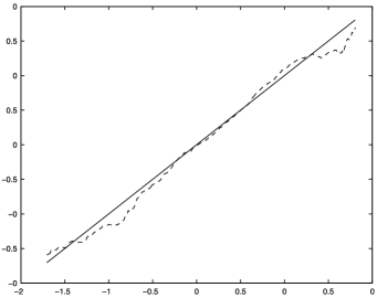
Figure 2: Nonparametric estimate of the regression function $g_{0}(v)$ for the case of $H(v)\equiv 0$ with sample size $n=700$; the solid line is the true line, and the dashed curve is the estimated curve.

It is easy to check that the random walk $\{V_{t}\}$ defined in this example corresponds to a $1/2$ null recurrent process and the assumptions in Section 2 are satisfied here. We choose sample sizes $n=200,700,1200$ and $N=1000$ as the number of replications in the simulation. The simulation results are listed in Tables 1 and 2 and the plots are given in Figures 1–6.

Figure 3: Nonparametric estimate of the regression function $g_{0}(v)$ for the case of $H(v)\equiv 0$ with sample size $n=1200$; the solid line is the true line, and the dashed curve is the estimated curve.

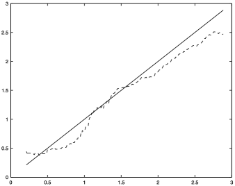
Figure 4: Nonparametric estimate of the regression function $g_{0}(v)$ for the case of $H(v)=v$ with sample size $n=200$; the solid line is the true line, and the dashed curve is the estimated curve.

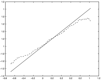
Figure 5: Nonparametric estimate of the regression function $g_{0}(v)$ for the case of $H(v)=v$ with sample size $n=700$; the solid line is the true line, and the dashed curve is the estimated curve.

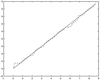
Figure 6: Nonparametric estimate of the regression function $g_{0}(v)$ for the case of $H(v)=v$ with sample size $n=1200$; the solid line is the true line, and the dashed curve is the estimated curve.

The performance of $\widehat{\theta}_{n}$ is given in Table 1. The “AE” in Table 1 is defined by $\frac{1}{1000}\sum_{j=1}^{1000}|\widehat{\theta}(j)-\theta_{0}|$, where $\widehat{\theta}(j)$ is the value of $\widehat{\theta}_{n}$ in the $j$th replication. “SE” is the standard error of $\{\widehat{\theta}(j)\}$. From Table 1, we find that the estimator of $\theta_{0}$ performs well in the small and medium sample cases and it improves when the sample size increases.

The performance of the nonparametric estimator is given in Table 2. The “AE” in Table 2 is the mean of the absolute errors in 1000 replications. The absolute error is defined by $\frac{1}{300}\sum_{j=1}^{300}|\widehat{g}_{n}(v_{j})-v_{j}|$, where $v_{j}=v_{\min}+\frac{j-1}{300}(v_{\max}-v_{\min})$ for $j=1,2,\ldots,300$, $v_{\max}$ and $v_{\min}$ are the maximum and minimum of the random walk $\{V_{t},1\leq t\leq n\}$, respectively. “SE” in Table 2 is the standard error. From Table 2, we find that the nonparametric estimate of $g_{0}(v)=v$ performs well in our example and it improves when the sample size increases.

Figures 1–3 compare the true nonparametric regression function $g_{0}(\cdot)$ and its nonparametric estimator for the case of $H(v)=0$ when the sample sizes are 200, 700 and 1200, respectively. Figures 4–6 compare the true nonparametric regression function $g_{0}(\cdot)$ with its nonparametric estimator for the case of $H(v)=v$ when the sample sizes are 200, 700 and 1200, respectively. The solid line is $g_{0}(\cdot)$ and the dashed line is the nonparametric estimator. We cannot forecast the trace of the random walk $\{V_{t}\}$ because of its non-stationarity. Hence, we estimate the true regression function $g_{0}(\cdot)$ according to the scope of $\{V_{t}\}$ and we cannot estimate $g_{0}(\cdot)$ in other points out of the scope since there is not enough sample in the neighborhood of each of such points. That is why the scopes of the abscissa axis are different in Figures 1–6. We can also find that the performance of the nonparametric estimate of $g_{0}(\cdot)$ improves as the sample size increases.

5 An empirical application

We use monthly observations on the U.S. share price indices, long-term government bond yields and treasury bill rates from Jan/1957–Dec/2009. The data are obtained from the International Monetary Fund’s (IMF) International Financial Statistics (IFS). The share price series used is IFS Series 11162ZF. The long-term government bond yield, which is the 10-year yield, is from the IFS Series 11161ZF. The treasury bill rate is from IFS Series 11160CZF. Figure 7(a)–(c) gives the data plots of the share prices, the long-term bond yields and the treasury bill rates.

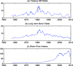
Figure 7: Time plots of the three series used in Section 5 over the period of Jan/1957–Dec/2009 with 624 observations. (a) treasury bill rates; (b) long-term bond yields; (c) share prices.

To see whether there exist some statistical evidences for the three series to have the unit root type of non-stationarity, we carry out a Dickey–Fuller (DF) unit root test on the three series. We first fit the data by an $\operatorname{AR}(1)$ model of the form

$$Z_{t}=\rho Z_{t-1}+e_{t},$$

where $Z_{t}=$ share price at time $t$ or long-term bond yield at time $t$ or treasury bill rate at time $t$. Then, by using the least-squares estimation method, we estimate the parameter $\rho$ for the three series: for the share price series, $\widehat{\rho}_{\rm share}=1.0023$; for the long-term bond yield series, $\widehat{\rho}_{\mathrm{Lbond}}=0.9992$; and for the treasury bill rate series, $\widehat{\rho}_{\mathrm{Tbill}}=0.9966$. Then we calculate the Dickey–Fuller $t$ statistics and compare them with the critical values at the $5\%$ significance level. The simulated $P$ values for the long-term bond yields, treasury bill rates and share prices are $0.7040$, $0.3130$ and $0.4410$, respectively. In addition, we also employ an augmented DF test and the nonparametric test proposed in Gao et al. [11] for checking the unit root structure of $\{Z_{t}\}$. The resulting $P$ values are very similar to those obtained above.

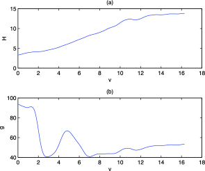
Figure 8: Estimates of the nonparametric functions $H(\cdot)$ and $g(\cdot)$ in Case A.

Therefore, both the estimation results and the simulated $P$ values suggest that there is some strong evidence for accepting the null hypothesis that a unit root structure exists in these series at the $5\%$ significance level.

We then consider the following modelling problem:

$$Y_{t} = X_{t}\theta_{0}+g(V_{t})+\epsilon_{t},$$

$$X_{t} = H(V_{t})+U_{t},$$

where Case A: $Y_{t}$ is the share price, $X_{t}$ is the long-term bond yield and $V_{t}$ is the treasury bill; and Case B: $Y_{t}$ is the long-term bond yield, $X_{t}$ is the share price and $V_{t}$ is the treasury bill.

For Case A, the resulting estimator of $\theta_{0}$ is $\widehat{\theta}=-3.2155$ and the plots of the estimates of $g(\cdot)$ and $H(\cdot)$ are given in Figure 8. For Case B, the resulting estimator of $\theta_{0}$ is $\widehat{\theta}=-0.0037$ and the the plots of the estimates of $g(\cdot)$ and $H(\cdot)$ are given in Figure 9.

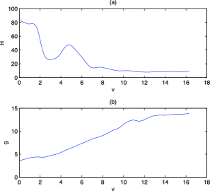
Figure 9: Estimates of the nonparametric functions $H(\cdot)$ and $g(\cdot)$ in Case B.

Figures 8 and 9 show that increases in treasury bill rates tend to lead to increases in long-term bond yields and decreases in share prices. Such findings are supported by the theory of finance and consistent with existing studies. Moreover, Figures 7–9 clearly indicate our new findings that both null recurrent non-stationarity and nonlinearity can be simultaneously exhibited in the share price, the long-term bond yield and the treasury bill rate variables.

Due to the cointegrating relationship among the stock price, the treasury bill rate and the long-term bond yield variables, our experience suggests that models (3.2) and (3.2) might be more suitable for this empirical study. We will have another look at this data after models (3.2) and (3.2) have been fully studied.

6 An outline of the proofs of the theorems

In this section, we provide only one key lemma and then an outline of the proofs of Theorems 5 and 8. The detailed proofs of the theorems are available from the supplemental document by Chen, Gao and Li [5].

Lemma 6.0

Under the conditions of Theorem 5, we have as $n\rightarrow\infty$,

$$\frac{1}{n}\widetilde{X}^{\tau}\widetilde{X}\stackrel{{\scriptstyle P}}{{\longrightarrow}}\Sigma.$$ (36)

Proof of Theorem 5 In view of Lemma 10 and the decomposition

$$\widetilde{X}^{\tau}\widetilde{X}(\widehat{\theta}_{n}-\theta_{0}) = \widetilde{X}^{\tau}(\widetilde{Y}-\widetilde{X}\theta_{0})$$

$$= \sum_{t=1}^{n}\widetilde{X}_{t}\widetilde{g}(V_{t})F_{t}+\sum_{t=1}^{n}\widetilde{X}_{t}\epsilon_{t}F_{t}-\sum_{t=1}^{n}\widetilde{X}_{t}F_{t}\Biggl{(}\sum_{k=1}^{n}w_{nk}(V_{t})\epsilon_{k}\Biggr{)},$$

in order to prove Theorem 5, we need only to show that for large enough $n$

$$\sum_{t=1}^{n}\widetilde{X}_{t}\widetilde{g}(V_{t})F_{t} = \mathrm{o}_{P}\bigl{(}\sqrt{n}\bigr{)},$$ (37)

$$\sum_{t=1}^{n}\widetilde{X}_{t}F_{t}\Biggl{\{}\sum_{k=1}^{n}w_{nk}(V_{t})\epsilon_{k}\Biggr{\}} = \mathrm{o}_{P}\bigl{(}\sqrt{n}\bigr{)},$$ (38)

$$n^{-1/2}\sum_{t=1}^{n}\widetilde{X}_{t}\epsilon_{t}F_{t} \stackrel{{\scriptstyle d}}{{\longrightarrow}} N(0,\Sigma_{\epsilon,U}),$$ (39)

where $\widetilde{g}(V_{t})=g(V_{t})-\sum_{k=1}^{n}w_{nk}(V_{t})g(V_{k})$. Recall that $\widetilde{X}_{t}=X_{t}-\sum_{s=1}^{n}w_{ns}(V_{t})X_{s}=U_{t}-\sum_{s=1}^{n}w_{ns}(V_{t})U_{s}+\widetilde{H}(V_{t})$, where $\widetilde{H}(V_{t})=H(V_{t})-\sum_{s=1}^{n}w_{ns}(V_{t})H(V_{s})$.

In order to prove (37)–(39), it suffices to show that for large enough $n$

$$\sum_{t=1}^{n}U_{t}\widetilde{g}(V_{t})F_{t} = \mathrm{o}_{P}\bigl{(}\sqrt{n}\bigr{)},$$ (40)

$$\sum_{t=1}^{n}\overline{U}_{t}\widetilde{g}(V_{t})F_{t} = \mathrm{o}_{P}\bigl{(}\sqrt{n}\bigr{)},$$ (41)

$$\sum_{t=1}^{n}\widetilde{g}(V_{t})\widetilde{H}(V_{t})F_{t} = \mathrm{o}_{P}\bigl{(}\sqrt{n}\bigr{)},$$ (42)

$$\sum_{t=1}^{n}U_{t}\overline{\epsilon}_{t}F_{t} = \mathrm{o}_{P}\bigl{(}\sqrt{n}\bigr{)},$$ (43)

$$\sum_{t=1}^{n}\overline{U}_{t}\overline{\epsilon}_{t}F_{t} = \mathrm{o}_{P}\bigl{(}\sqrt{n}\bigr{)},$$ (44)

$$\sum_{t=1}^{n}\widetilde{H}(V_{t})\overline{\epsilon}_{t}F_{t} = \mathrm{o}_{P}\bigl{(}\sqrt{n}\bigr{)},$$ (45)

$$\sum_{t=1}^{n}\overline{U}_{t}\epsilon_{t}F_{t} = \mathrm{o}_{P}\bigl{(}\sqrt{n}\bigr{)},$$ (46)

$$\sum_{t=1}^{n}\widetilde{H}(V_{t})\epsilon_{t}F_{t} = \mathrm{o}_{P}\bigl{(}\sqrt{n}\bigr{)},$$ (47)

$$n^{-1/2}\sum_{t=1}^{n}U_{t}\epsilon_{t}F_{t} \stackrel{{\scriptstyle d}}{{\longrightarrow}} N(0,\Sigma_{\epsilon,U}),\vspace*{-2pt}$$ (48)

where $\overline{U}_{t}=\sum_{s=1}^{n}w_{ns}(V_{t})U_{s}$ and $\overline{\epsilon}_{t}=\sum_{s=1}^{n}w_{ns}(V_{t})\epsilon_{s}$.

In the following, we verify equations (40)–(48) to complete the proofs of Theorem 5(i) and Theorem 5(ii). Note that, for Theorem 5(i), equations (42), (45) and (47) hold trivially.

By the continuity of $g(\cdot)$ and $g^{\prime}(\cdot)$, we have for $1\leq t\leq n$,

$$\frac{1}{N(n)h}\sum_{j=1}^{n}K\biggl{(}\frac{V_{j}-V_{t}}{h}\biggr{)}\bigl{(}g(V_{j})-g(V_{t})\bigr{)}$$

(49)

$$\quad=\frac{g^{\prime}(V_{t})}{N(n)h}\sum_{j=1}^{n}(V_{j}-V_{t})K\biggl{(}\frac{V_{j}-V_{t}}{h}\biggr{)}\bigl{(}1+\mathrm{o}_{P}(1)\bigr{)}.\vspace*{-2pt}$$

Thus, in view of (6) and Lemma 3.4 of Karlsen and Tjøstheim [20], in order to prove (40), it suffices to show that for $n$ large enough

$$\sum_{t=1}^{n}U_{t}\Delta_{n}(V_{t})F_{t}=\mathrm{o}_{P}\bigl{(}\sqrt{n}\bigr{)},\vspace*{-2pt}$$ (50)

where $\Delta_{n}(V_{t})=\frac{g^{\prime}(V_{t})}{n^{\beta-\eta}hp_{n}(V_{t})}\sum_{j=1}^{n}(V_{j}-V_{t})K(\frac{V_{j}-V_{t}}{h})$.

This kind of procedure of replacing $N(n)$ by $n^{\beta-\eta}$ and ignoring a small-order term as involved in (6) will be used repeatedly throughout the proofs in Appendices B and C of the supplemental document.

We then may show that (41) holds. Similarly to (6) and (50), we need only to show that

$$\sum_{t=1}^{n}\widehat{U}_{t}\Delta_{n}(V_{t})F_{t}=\mathrm{o}_{P}\bigl{(}\sqrt{n}\bigr{)},\vspace*{-2pt}$$ (51)

where $\widehat{U}_{t}=\frac{1}{n^{\beta-\eta}hp_{n}(V_{t})}(\sum_{k=1}^{n}K(\frac{V_{k}-V_{t}}{h})U_{k})$.

The detailed derivations for (50) and (51) are available from Appendix B of the supplemental document. The detailed proofs of (43), (44), (46) and (48) are also available from Appendix B. This will complete the proof of Theorem 5(i).

We then may prove Theorem 5(ii) by completing the proofs of (42), (45) and (47), which are again available from Appendix B of the supplemental document. Proof of Theorem 8 By the definition of $\widehat{g}_{n}(v)$, we have

$$\widehat{g}_{n}(v)-g(v) = \sum_{t=1}^{n}w_{nt}(v)(Y_{t}-X_{t}\widehat{\theta}_{n})-g(v)$$

$$= \sum_{t=1}^{n}w_{nt}(v)\bigl{(}\epsilon_{t}+g(V_{t})-g(v)\bigr{)}+\sum_{t=1}^{n}w_{nt}(v)X_{t}(\theta_{0}-\widehat{\theta}_{n}).\vspace*{-2pt}$$

Let $\Phi_{n,1}=\sum_{t=1}^{n}w_{nt}(v)(\epsilon_{t}+g(V_{t})-g(v)$ and $\Phi_{n,2}=\sum_{t=1}^{n}w_{nt}(v)X_{t}(\theta_{0}-\widehat{\theta}_{n})$. Then, we have

$$\widehat{g}_{n}(v)-g(v) = \sum_{t=1}^{n}w_{nt}(v)(Y_{t}-X_{t}\widehat{\theta}_{n})-g(v)=\Phi_{n,1}+\Phi_{n,2}.$$ (53)

Since $\{\epsilon_{t}\}$ is assumed to be stationary and $\alpha$ mixing, by Corollary 5.1 of Hall and Heyde [14] and an existing technique to deal with the bias term (see, e.g., the proof of Theorem 3.5 of Karlsen et al. [19]), we have as $n\rightarrow\infty$

$$\sqrt{\sum_{t=1}^{n}K\biggl{(}\frac{V_{t}-v}{h}\biggr{)}}\Phi_{n,1}\stackrel{{\scriptstyle d}}{{\longrightarrow}}N\biggl{(}0,\sigma^{2}\int K^{2}(u)\,\mathrm{d}u\biggr{)}.$$ (54)

By (6)–(54), it is sufficient to show that

$$\sqrt{\sum_{t=1}^{n}K\biggl{(}\frac{V_{t}-v}{h}\biggr{)}}\Phi_{n,2}=\mathrm{o}_{P}(1).$$ (55)

The proof of (55) may then be completed by Theorem 5 and Assumptions A1–A6. The details are available from Appendix B of the supplemental document. This completes an outline of the proofs of Theorems 5 and 8.

References

- [1] {barticle}[mr] \bauthor\bsnmBandi, \bfnmFederico M.\binitsF.M. &\bauthor\bsnmPhillips, \bfnmPeter C. B.\binitsP.C.B. (\byear2003). \btitleFully nonparametric estimation of scalar diffusion models. \bjournalEconometrica \bvolume71 \bpages241–283. \biddoi=10.1111/1468-0262.00395, issn=0012-9682, mr=1956859 \endbibitem
- [2] {barticle}[mr] \bauthor\bsnmBhattacharya, \bfnmP. K.\binitsP.K. &\bauthor\bsnmZhao, \bfnmPeng-Liang\binitsP.L. (\byear1997). \btitleSemiparametric inference in a partial linear model. \bjournalAnn. Statist. \bvolume25 \bpages244–262. \biddoi=10.1214/aos/1034276628, issn=0090-5364, mr=1429924 \endbibitem
- [3] {bbook}[mr] \bauthor\bsnmBickel, \bfnmPeter J.\binitsP.J., \bauthor\bsnmKlaassen, \bfnmChris A. J.\binitsC.A.J., \bauthor\bsnmRitov, \bfnmYa’acov\binitsY. &\bauthor\bsnmWellner, \bfnmJon A.\binitsJ.A. (\byear1993). \btitleEfficient and Adaptive Estimation for Semiparametric Models. \baddressBaltimore, MD: \bpublisherJohns Hopkins Univ. Press. \bidmr=1245941 \endbibitem
- [4] {barticle}[mr] \bauthor\bsnmChen, \bfnmHung\binitsH. (\byear1988). \btitleConvergence rates for parametric components in a partly linear model. \bjournalAnn. Statist. \bvolume16 \bpages136–146. \biddoi=10.1214/aos/1176350695, issn=0090-5364, mr=0924861 \endbibitem
- [5] {bmisc}[auto:STB—2011-03-03—12:04:44] \bauthor\bsnmChen, \bfnmJ.\binitsJ., \bauthor\bsnmGao, \bfnmJ.\binitsJ. &\bauthor\bsnmLi, \bfnmD.\binitsD. (\byear2010). \bhowpublishedSupplement to “Estimation in semi-parametric regression with non-stationary regressors.” DOI: 10.3150/10-BEJ344SUPP. \endbibitem
- [6] {bincollection}[mr] \bauthor\bsnmChen, \bfnmX.\binitsX. (\byear2007). \btitleLarge sample sieve estimation of semi–nonparametric models. In \bbooktitleHandbook of Econometrics \bvolumeVI (\beditor\bfnmJ. J.\binitsJ.J. \bsnmHeckman &\beditor\bfnmE. E.\binitsE.E. \bsnmLeamer, eds.) \bpages5549–5632. \baddressAmsterdam: \bpublisherElsevier. \endbibitem
- [7] {barticle}[auto:STB—2011-03-03—12:04:44] \bauthor\bsnmEngle, \bfnmR.\binitsR., \bauthor\bsnmGranger, \bfnmC.\binitsC., \bauthor\bsnmRice, \bfnmJ.\binitsJ. &\bauthor\bsnmWeiss, \bfnmA.\binitsA. (\byear1986). \btitleSemiparametric estimates of the relation between weather and electricity sales. \bjournalJ. Amer. Statist. Assoc. \bvolume81 \bpages310–320. \endbibitem
- [8] {bbook}[mr] \bauthor\bsnmFan, \bfnmJ.\binitsJ. &\bauthor\bsnmGijbels, \bfnmI.\binitsI. (\byear1996). \btitleLocal Polynomial Modelling and Its Applications. \bseriesMonographs on Statistics and Applied Probability \bvolume66. \baddressLondon: \bpublisherChapman and Hall. \bidmr=1383587 \endbibitem
- [9] {bbook}[mr] \bauthor\bsnmFan, \bfnmJianqing\binitsJ. &\bauthor\bsnmYao, \bfnmQiwei\binitsQ. (\byear2003). \btitleNonlinear Time Series. Nonparametric and Parametric Methods. \baddressNew York: \bpublisherSpringer. \biddoi=10.1007/b97702, mr=1964455 \endbibitem
- [10] {bbook}[mr] \bauthor\bsnmGao, \bfnmJiti\binitsJ. (\byear2007). \btitleNonlinear Time Series. Semiparametric and Nonparametric Methods. \bseriesMonographs on Statistics and Applied Probability \bvolume108. \baddressBoca Raton, FL: \bpublisherChapman and Hall/CRC. \biddoi=10.1201/9781420011210, mr=2297190 \endbibitem
- [11] {barticle}[mr] \bauthor\bsnmGao, \bfnmJiti\binitsJ., \bauthor\bsnmKing, \bfnmMaxwell\binitsM., \bauthor\bsnmLu, \bfnmZudi\binitsZ. &\bauthor\bsnmTjøstheim, \bfnmDag\binitsD. (\byear2009). \btitleNonparametric specification testing for nonlinear time series with nonstationarity. \bjournalEconometric Theory \bvolume25 \bpages1869–1892. \biddoi=10.1017/S0266466609990363, issn=0266-4666, mr=2557585 \endbibitem
- [12] {barticle}[auto:STB—2011-03-03—12:04:44] \bauthor\bsnmGao, \bfnmJ.\binitsJ., \bauthor\bsnmKing, \bfnmM. L.\binitsM.L., \bauthor\bsnmLu, \bfnmZ.\binitsZ. &\bauthor\bsnmTjøstheim, \bfnmD.\binitsD. (\byear2009). \btitleSpecification testing in nonstationary time series autoregression. \bjournalAnn. Statist. \bvolume37 \bpages3893–3928. \endbibitem
- [13] {bbook}[mr] \bauthor\bsnmGreen, \bfnmP. J.\binitsP.J. &\bauthor\bsnmSilverman, \bfnmB. W.\binitsB.W. (\byear1994). \btitleNonparametric Regression and Generalized Linear Models: A Roughness Penalty Approach. \bseriesMonographs on Statistics and Applied Probability \bvolume58. \baddressLondon: \bpublisherChapman & Hall. \bidmr=1270012 \bptokimsref \endbibitem
- [14] {bbook}[mr] \bauthor\bsnmHall, \bfnmP.\binitsP. &\bauthor\bsnmHeyde, \bfnmC. C.\binitsC.C. (\byear1980). \btitleMartingale Limit Theory and Its Application. \baddressNew York: \bpublisherAcademic Press. \bidmr=0624435 \endbibitem
- [15] {bbook}[mr] \bauthor\bsnmHärdle, \bfnmWolfgang\binitsW., \bauthor\bsnmLiang, \bfnmHua\binitsH. &\bauthor\bsnmGao, \bfnmJiti\binitsJ. (\byear2000). \btitlePartially Linear Models. \baddressHeidelberg: \bpublisherPhysica-Verlag. \bidmr=1787637 \endbibitem
- [16] {barticle}[author] \bauthor\bsnmHärdle, \bfnmW.\binitsW., \bauthor\bsnmLütkepohl, \bfnmH.\binitsH. &\bauthor\bsnmChen, \bfnmR.\binitsR. (\byear1997). \btitleA review of nonparametric time series analysis. \bjournalInternat. Statist. Rev. \bvolume65 \bpages49–72. \endbibitem
- [17] {bbook}[mr] \bauthor\bsnmHastie, \bfnmT. J.\binitsT.J. &\bauthor\bsnmTibshirani, \bfnmR. J.\binitsR.J. (\byear1990). \btitleGeneralized Additive Models. \bseriesMonographs on Statistics and Applied Probability \bvolume43. \baddressLondon: \bpublisherChapman and Hall. \bidmr=1082147 \endbibitem
- [18] {barticle}[mr] \bauthor\bsnmJuhl, \bfnmTed\binitsT. &\bauthor\bsnmXiao, \bfnmZhijie\binitsZ. (\byear2005). \btitlePartially linear models with unit roots. \bjournalEconometric Theory \bvolume21 \bpages877–906. \biddoi=10.1017/S0266466605050450, issn=0266-4666, mr=2168183 \endbibitem
- [19] {barticle}[mr] \bauthor\bsnmKarlsen, \bfnmHans Arnfinn\binitsH.A., \bauthor\bsnmMyklebust, \bfnmTerje\binitsT. &\bauthor\bsnmTjøstheim, \bfnmDag\binitsD. (\byear2007). \btitleNonparametric estimation in a nonlinear cointegration type model. \bjournalAnn. Statist. \bvolume35 \bpages252–299. \biddoi=10.1214/009053606000001181, issn=0090-5364, mr=2332276 \endbibitem
- [20] {barticle}[mr] \bauthor\bsnmKarlsen, \bfnmHans Arnfinn\binitsH.A. &\bauthor\bsnmTjøstheim, \bfnmDag\binitsD. (\byear2001). \btitleNonparametric estimation in null recurrent time series. \bjournalAnn. Statist. \bvolume29 \bpages372–416. \biddoi=10.1214/aos/1009210546, issn=0090-5364, mr=1863963 \endbibitem
- [21] {bbook}[mr] \bauthor\bsnmLi, \bfnmQi\binitsQ. &\bauthor\bsnmRacine, \bfnmJeffrey Scott\binitsJ.S. (\byear2007). \btitleNonparametric Econometrics. Theory and Practice. \baddressPrinceton, NJ: \bpublisherPrinceton Univ. Press. \bidmr=2283034 \endbibitem
- [22] {bbook}[mr] \bauthor\bsnmLin, \bfnmZhengyan\binitsZ. &\bauthor\bsnmLu, \bfnmChuanrong\binitsC. (\byear1996). \btitleLimit Theory for Mixing Dependent Random Variables. \bseriesMathematics and Its Applications \bvolume378. \baddressDordrecht: \bpublisherKluwer Academic. \bidmr=1486580 \endbibitem
- [23] {barticle}[mr] \bauthor\bsnmLinton, \bfnmOliver\binitsO. (\byear1995). \btitleSecond order approximation in the partially linear regression model. \bjournalEconometrica \bvolume63 \bpages1079–1112. \biddoi=10.2307/2171722, issn=0012-9682, mr=1348514 \endbibitem
- [24] {bbook}[mr] \bauthor\bsnmNummelin, \bfnmEsa\binitsE. (\byear1984). \btitleGeneral Irreducible Markov Chains and Nonnegative Operators. \bseriesCambridge Tracts in Mathematics \bvolume83. \baddressCambridge: \bpublisherCambridge Univ. Press. \biddoi=10.1017/CBO9780511526237, mr=0776608 \bptokimsref \endbibitem
- [25] {bmisc}[auto:STB—2011-03-03—12:04:44] \bauthor\bsnmPhillips, \bfnmP. C. B.\binitsP.C.B. &\bauthor\bsnmPark, \bfnmJ.\binitsJ. (\byear1998). \bhowpublishedNonstationary density estimation and kernel autoregression. Cowles Foundation Discussion Paper No. 1181, Yale Univ. \endbibitem
- [26] {barticle}[mr] \bauthor\bsnmRobinson, \bfnmP. M.\binitsP.M. (\byear1983). \btitleNonparametric estimators for time series. \bjournalJ. Time Ser. Anal. \bvolume4 \bpages185–207. \biddoi=10.1111/j.1467-9892.1983.tb00368.x, issn=0143-9782, mr=0732897 \endbibitem
- [27] {barticle}[mr] \bauthor\bsnmRobinson, \bfnmP. M.\binitsP.M. (\byear1988). \btitleRoot--consistent semiparametric regression. \bjournalEconometrica \bvolume56 \bpages931–954. \biddoi=10.2307/1912705, issn=0012-9682, mr=0951762 \endbibitem
- [28] {barticle}[mr] \bauthor\bsnmRobinson, \bfnmP. M.\binitsP.M. (\byear1989). \btitleHypothesis testing in semiparametric and nonparametric models for econometric time series. \bjournalRev. Econom. Stud. \bvolume56 \bpages511–534. \biddoi=10.2307/2297498, issn=0034-6527, mr=1023837 \endbibitem
- [29] {barticle}[mr] \bauthor\bsnmRosenblatt, \bfnmM.\binitsM. (\byear1956). \btitleA central limit theorem and a strong mixing condition. \bjournalProc. Natl. Acad. Sci. U.S.A. \bvolume42 \bpages43–47. \bidissn=0027-8424, mr=0074711 \endbibitem
- [30] {bmisc}[auto:STB—2011-03-03—12:04:44] \bauthor\bsnmSchienle, \bfnmM.\binitsM. (\byear2008). \bhowpublishedNonparametric nonstationary regression. Working paper, Department of Economics, Univ. Mannheim, Germany. \endbibitem
- [31] {bbook}[mr] \bauthor\bsnmSilverman, \bfnmB. W.\binitsB.W. (\byear1986). \btitleDensity Estimation for Statistics and Data Analysis. \baddressLondon: \bpublisherChapman and Hall. \bidmr=0848134 \endbibitem
- [32] {barticle}[mr] \bauthor\bsnmWang, \bfnmQiying\binitsQ. &\bauthor\bsnmPhillips, \bfnmPeter C. B.\binitsP.C.B. (\byear2009). \btitleAsymptotic theory for local time density estimation and nonparametric cointegrating regression. \bjournalEconometric Theory \bvolume25 \bpages710–738. \biddoi=10.1017/S0266466608090269, issn=0266-4666, mr=2507529 \endbibitem
- [33] {barticle}[mr] \bauthor\bsnmWang, \bfnmQiying\binitsQ. &\bauthor\bsnmPhillips, \bfnmPeter C. B.\binitsP.C.B. (\byear2009). \btitleStructural nonparametric cointegrating regression. \bjournalEconometrica \bvolume77 \bpages1901–1948. \biddoi=10.3982/ECTA7732, issn=0012-9682, mr=2573873 \endbibitem
- [34] {barticle}[mr] \bauthor\bsnmWithers, \bfnmC. S.\binitsC.S. (\byear1981). \btitleConditions for linear processes to be strong-mixing. \bjournalZ. Wahrsch. Verw. Gebiete \bvolume57 \bpages477–480. \biddoi=10.1007/BF01025869, issn=0044-3719, mr=0631371 \endbibitem