Non-D-finite excursions in the quarter plane

Abstract.

The number of excursions (finite paths starting and ending at the origin) having a given number of steps and obeying various geometric constraints is a classical topic of combinatorics and probability theory. We prove that the sequence $(e^{\mathfrak{S}}_{n})_{n\geq 0}$ of numbers of excursions in the quarter plane corresponding to a nonsingular step set $\mathfrak{S}\subseteq\{0,\pm 1\}^{2}$ with infinite group does not satisfy any nontrivial linear recurrence with polynomial coefficients. Accordingly, in those cases, the trivariate generating function of the numbers of walks with given length and prescribed ending point is not D-finite. Moreover, we display the asymptotics of $e^{\mathfrak{S}}_{n}$.

1. Introduction

1.1. General context

Counting walks in a fixed region of the lattice $\mathbb{Z}^{d}$ is a classical problem in probability theory [1, 2, 3, 4, 5, 6, 7, 8, 9, 10] and in enumerative combinatorics [11, 12, 13]. In recent years, the case of walks restricted to the quarter plane $\mathbb{N}^{2}=\{(i,j)\in\mathbb{Z}^{2}\,|\,i\geq 0,\,j\geq 0\}$ has received special attention, and much progress has been done on this topic [14, 15, 16, 17, 18, 19, 20, 21, 22, 23, 24, 25, 26, 27, 28, 29, 31, 32, 33, 34, 35, 36, 30, 38, 39, 37]. Given a finite set $\mathfrak{S}$ of allowed steps, the general problem is to study $\mathfrak{S}$-walks in the quarter plane $\mathbb{N}^{2}$, that is walks confined to $\mathbb{N}^{2}$, starting at $(0,0)$ and using steps in $\mathfrak{S}$ only. Denoting by $f_{\mathfrak{S}}(i,j,n)$ the number of such walks that end at $(i,j)$ and use exactly $n$ steps, the main high-level objective is to understand the generating function

$$F_{\mathfrak{S}}(x,y,t)=\sum_{i,j,n\geq 0}f_{\mathfrak{S}}(i,j,n)x^{i}y^{j}t^{n}\;\in\mathbb{Q}[[x,y,t]],$$

since this continuous object captures a great amount of interesting combinatorial information about the discrete object $f_{\mathfrak{S}}(i,j,n)$. For instance, the specialization $F_{\mathfrak{S}}(1,1,t)$ is the generating function of the numbers of ${\mathfrak{S}}$-walks with prescribed length, the specialization $F_{\mathfrak{S}}(1,0,t)$ is that of ${\mathfrak{S}}$-walks ending on the horizontal axis, and the specialization $F_{\mathfrak{S}}(0,0,t)$ counts ${\mathfrak{S}}$-walks returning to the origin, called ${\mathfrak{S}}$-excursions.

1.2. Questions

From the combinatorial point of view, the ideal goal would be to find a closed-form expression for $f_{\mathfrak{S}}(i,j,n)$, or at least for $F_{\mathfrak{S}}(x,y,t)$. This is not possible in general, even if one restricts to particular step sets $\mathfrak{S}$. Therefore, it is customary to address more modest, still challenging, questions such as: What is the asymptotic behavior of the sequence $f_{\mathfrak{S}}(i,j,n)$? What are the structural properties of $F_{\mathfrak{S}}(x,y,t)$: is it rational? is it algebraic? or more generally D-finite? These questions are related, since the asymptotic behavior of the coefficient sequence of a power series is well understood for rational, algebraic and D-finite power series [41, Part B].

1.3. Main result

In this work, we prove that the generating function

$$F_{\mathfrak{S}}(0,0,t)=\sum_{n\geq 0}e^{\mathfrak{S}}_{n}t^{n}\;\in\mathbb{Q}[[t]]$$

of the sequence $(e^{\mathfrak{S}}_{n})_{n\geq 0}$ of ${\mathfrak{S}}$-excursions is not D-finite for a large class of walks in the quarter plane. Precisely, this large class corresponds to all small-step sets $\mathfrak{S}\subseteq\{0,\pm 1\}^{2}{\setminus\{0,0\}}$ for which a certain group $G_{\mathfrak{S}}$ of birational transformations is infinite, with the exception of a few cases for which $F_{\mathfrak{S}}(0,0,t)=1$ is trivially D-finite (these exceptional cases are called singular, see below). If $\chi=\chi_{\mathfrak{S}}$ denotes the characteristic polynomial of the step set $\mathfrak{S}$ defined by

$$\chi(x,y)=\sum_{(i,j)\in\mathfrak{S}}x^{i}y^{j}\;\in\mathbb{Q}[x,x^{-1},y,y^{-1}],$$

then the group $G_{\mathfrak{S}}$ is defined [18, 28] as a group of rational automorphisms of $\mathbb{Q}(x,y)$ that leave invariant the (Laurent) polynomial $\chi(x,y)$. Up to some equivalence relations, there are 74 cases of nonsingular step sets in $\mathbb{N}^{2}$, out of which 51 cases have an infinite group [28]. These 51 cases are depicted in Table 4 in Appendix 4. With these definitions, our main result can be stated as follows.

Theorem 1.

Let $\mathfrak{S}\subseteq\{0,\pm 1\}^{2}$ be any of the 51 nonsingular step sets in $\mathbb{N}^{2}$ with infinite group $G_{\mathfrak{S}}$. Then the generating function $F_{\mathfrak{S}}(0,0,t)$ of ${\mathfrak{S}}$-excursions is not D-finite. Equivalently, the excursion sequence $(e^{\mathfrak{S}}_{n})_{n\geq 0}$ does not satisfy any nontrivial linear recurrence with polynomial coefficients. In particular, the full generating function $F_{\mathfrak{S}}(x,y,t)$ is not D-finite.

By combining Theorem 1 with previously known results, we obtain the following characterization of nonsingular small-step sets with D-finite generating function.

Corollary 2.

Let $\mathfrak{S}\subseteq\{0,\pm 1\}^{2}$ be any of the 74 nonsingular step sets in $\mathbb{N}^{2}$. The following assertions are equivalent:

1. The full generating function $F_{\mathfrak{S}}(x,y,t)$ is D-finite;

2. the generating function $F_{\mathfrak{S}}(0,0,t)$ of ${\mathfrak{S}}$-excursions is D-finite;

3. the excursion sequence $e^{\mathfrak{S}}_{2n}$ is asymptotically equivalent to $K\cdot\rho^{n}\cdot n^{\alpha}$, for some $\alpha\in\mathbb{Q}$;

4. the group ${G}_{\mathfrak{S}}$ is finite;

5. the step set $\mathfrak{S}$ has either an axial symmetry, or a zero drift and cardinality different from 5.

Moreover, under (1)–(5), the cardinality of ${G}_{\mathfrak{S}}$ is equal to $2\cdot\min\left\{\ell\in\mathbb{N}^{\star}\,|\,\frac{\ell}{\alpha+1}\in\mathbb{Z}\right\}$.

Implication $(4)\Rightarrow(1)$ is a consequence of results in [28, 27], proofs of $(1)\Rightarrow(2)\Rightarrow(3)\Rightarrow(4)$ are given in the present article, and the equivalence of (2) and (5) is read off the tables in Appendix 4. Condition (5) seems unnatural, its purpose is to eliminate the three rotations of the “scarecrow” walk with step sets depicted in Figure 1, which have zero drift and non-D-finite generating functions. The observation on the cardinality seems new and interesting. It can be checked from the data [28, Tables 1–3].

  

Figure 1. Rotations of a scarecrow. These are the three step sets (30, 40, 42 in Table 4) of walks with zero drift that have a non-D-finite generating function.

1.4. Previous results

1.4.1. Structural properties

While it is known that unrestricted walks in $\mathbb{Z}^{2}$ have rational generating functions and walks restricted to a half-plane in $\mathbb{Z}^{2}$ have algebraic generating functions (see [42] and [20, Proposition 2]), a first intriguing result about walks in the quarter plane is that their generating functions need not be algebraic, and not even D-finite. For instance, Bousquet-Mélou and Petkovšek [20] proved that this is the case for the so-called knight walk starting at $(1,1)$ with $\mathfrak{S}=\{(2,-1),(-1,2)\}$. (Although this is not a walk with unit steps, it actually constitutes one of the initial motivations for the study of walks evolving in the quarter plane.) It was later shown by Mishna and Rechnitzer [26] that even if one restricts to small-step walks, where $\mathfrak{S}\subseteq\{0,\pm 1\}^{2}$, there exist step sets, such as $\mathfrak{S}=\{(-1,1),(1,1),(1,-1)\}$, for which the series $F_{\mathfrak{S}}(x,y,t)$ is not D-finite (but in those cases $F_{\mathfrak{S}}(0,0,t)=1$ is trivially D-finite).

In the remainder of this text, we restrict ourselves to small-step walks in the quarter plane. Several sporadic cases of small-step walks with D-finite generating functions have been known for a long time; the most famous ones are Kreweras’ walks [14, 21], with $\mathfrak{S}=\{(-1,0),(0,-1),(1,1)\}$, and Gouyou-Beauchamps’ walks [16], with $\mathfrak{S}=$$\{(1,0),(-1,0),(-1,1),(1,-1)\}$. A whole class of small-step walks with D-finite generating functions was first identified in [20, §2]: this class contains step sets that admit an axial symmetry. Another class, including $\mathfrak{S}=\{(0,1),(-1,0),(1,-1)\}$ and $\mathfrak{S}=\{(0,1),(-1,0),(1,-1),(0,-1),(1,0),(-1,1)\}$, corresponds to step sets that are left invariant by a Weyl group and whose walks are confined to a corresponding Weyl chamber [17].

A systematic classification of small-step walks with respect to the D-finiteness of $F_{\mathfrak{S}}(1,1,t)$ was then undertaken by Mishna [22, 25] for step sets of cardinality at most three. A complete, still conjectural, classification without this restriction was obtained by Bostan and Kauers [23] using computer algebra tools. Almost simultaneously, Bousquet-Mélou and Mishna [28] proved that among the $2^{8}$ possible cases of small-step walks in the quarter plane, there are exactly 79 inherently different cases. Among these, they identified 22 cases of step sets $\mathfrak{S}$ having a D-finite generating function $F_{\mathfrak{S}}(x,y,t)$.

A 23rd case, namely $\mathfrak{G}=\{(1,0),(-1,0),(1,1),(-1,-1)\}$, known as Gessel walks, is notoriously challenging. Its generating function for excursions, $F_{\mathfrak{G}}(0,0,t)$, was first proved to be D-finite by Kauers, Koutschan and Zeilberger [24], using computer algebra techniques. Then Bostan and Kauers [27] discovered and proved that the full generating function $F_{\mathfrak{G}}(x,y,t)$ is D-finite, and even algebraic, again using computer algebra. It was proved afterwards by Fayolle and Raschel [29] using a different approach that for any fixed value $t_{0}\in(0,1/4)$, the bivariate generating function $F_{\mathfrak{G}}(x,y,t_{0})$ for Gessel walks is algebraic over $\mathbb{R}(x,y)$, hence over $\mathbb{Q}(x,y)$. Very recently, a “purely human” (i.e., computer-free) proof of the algebraicity of the full generating function $F_{\mathfrak{G}}(x,y,t)$ was given by Bostan, Kurkova and Raschel [38].

Bousquet-Mélou and Mishna [28] showed that these 23 cases of step sets $\mathfrak{S}$ with D-finite generating function $F_{\mathfrak{S}}(x,y,t)$ correspond to walks possessing a finite group $G_{\mathfrak{S}}$. Informally speaking, the group of a walk is a notion that captures symmetries of the step set and that is used to generalize a classical technique in lattice combinatorics called the “reflection principle” [2, Ch. III.1].

Moreover, it was conjectured in [28] that the 56 remaining models with infinite group have non-D-finite generating functions $F_{\mathfrak{S}}(x,y,t)$. This was proved by Kurkova and Raschel [33] for the 51 nonsingular walks, that is, for walks having at least one step from the set $\{(-1,0),(-1,-1),(0,-1)\}$. This result is obtained as a consequence of the non-D-finiteness of this series as a function of $x,y$. We provide an alternative proof of this result by showing the non-D-finiteness of $F_{\mathfrak{S}}(0,0,t)$, about which nothing was known.

As for the singular walks, two out of the five cases were already shown to have non-D-finite generating functions by Mishna and Rechnitzer [26]. The last 3 cases of singular walks have a generating function $F_{\mathfrak{S}}(x,y,t)$ that has just been proved to be non-D-finite by Melczer and Mishna [36].

1.4.2. Closed-form expressions

Closed forms are known for generating functions of the walks named after Kreweras [14], Gouyou-Beauchamps [16] and Gessel [24, 27, 38]. Some other explicit formulas for $f_{\mathfrak{S}}(i,j,n)$ and for $F_{\mathfrak{S}}(x,y,t)$, or some of their specializations, have been obtained by Bousquet-Mélou and Mishna [28] in cases when $\mathfrak{S}$ admits a finite group. A different type of explicit expressions (integral representations) for the generating function of Gessel walks was obtained by Kurkova and Raschel [32]. Their approach was later generalized by Raschel [35] to all the 74 nonsingular walks. Finally, Bostan, Chyzak, van Hoeij, Kauers and Pech [37] used computer algebra tools to express all D-finite transcendental functions $F_{\mathfrak{S}}(x,y,t)$ by iterated integrals of Gaussian hypergeometric functions.

1.4.3. Asymptotics

Concerning asymptotics, conjectural results were given by Bostan and Kauers [23] for the coefficients of $F_{\mathfrak{S}}(1,1,t)$ when this function is D-finite. Some of these conjectures have been proved by Bousquet-Mélou and Mishna [28]. Explicit asymptotics for the coefficients of $F_{\mathfrak{S}}(0,0,t)$ and $F_{\mathfrak{S}}(1,1,t)$ were conjectured even in non-D-finite cases in some unpublished tables [43]. In a recent work, Denisov and Wachtel [30] have obtained explicit expressions for the asymptotics of excursions $F_{\mathfrak{S}}(0,0,t)$ in a much broader setting; in particular, their results provide (up to a constant) the dominating term in the asymptotics of the $n$-th coefficient of $F_{\mathfrak{S}}(0,0,t)$ in terms of the step set. Even more recently, Fayolle and Raschel [34] showed that the dominant singularities of $F_{\mathfrak{S}}(0,0,t)$, $F_{\mathfrak{S}}(1,0,t)$ and $F_{\mathfrak{S}}(1,1,t)$ are algebraic numbers, and announced more general and precise results about asymptotics of coefficients of $F_{\mathfrak{S}}(0,0,t)$, $F_{\mathfrak{S}}(1,0,t)$ and $F_{\mathfrak{S}}(1,1,t)$. Furthermore, a combinatorial approach is proposed by Johnson, Mishna and Yeats [39] that allows to find tight bounds on the dominant singularities of the latter generating functions.

2. Number Theory, Probability and Algorithms

2.1. Contributions

In the present work, we prove the non-D-finiteness of the generating function of ${\mathfrak{S}}$-excursions $F_{\mathfrak{S}}(0,0,t)$ for all 51 cases of nonsingular walks with infinite group. As a corollary, we deduce the non-D-finiteness of the full generating function $F_{\mathfrak{S}}(x,y,t)$ for those cases since D-finiteness is preserved by specialization at (0,0) [40]. This corollary has been already obtained by Kurkova and Raschel [33], but the approach here is at the same time simpler, and delivers a more accurate information. This new proof only uses asymptotic information about the coefficients of $F_{\mathfrak{S}}(0,0,t)$, and arithmetic information about the constrained behavior of the asymptotics of these coefficients when their generating function is D-finite. More precisely, we first make explicit consequences of the general results by Denisov and Wachtel [30] in the case of walks in the quarter plane. If $e_{n}=e^{\mathfrak{S}}_{n}$ denotes the number of ${\mathfrak{S}}$-excursions of length $n$ using only steps in $\mathfrak{S}$, this analysis implies that, when $n$ tends to infinity, $e_{n}$ behaves like $K\cdot\rho^{n}\cdot n^{\alpha}$, where $K=K(\mathfrak{S})>0$ is a real number, $\rho=\rho(\mathfrak{S})$ is an algebraic number, and $\alpha=\alpha(\mathfrak{S})$ is a real number such that $c=-\cos(\frac{\pi}{1+\alpha})$ is an algebraic number. Explicit real approximations for $\rho$, $\alpha$ and $c$ can be determined to arbitrary precision. Moreover, exact minimal polynomials of $\rho$ and $c$ can be determined algorithmically starting from the step set $\mathfrak{S}$. For the 51 cases of nonsingular walks with infinite group, this enables us to prove that the constant $\alpha=\alpha(\mathfrak{S})$ is not a rational number. The proof amounts to checking that some explicit polynomials in $\mathbb{Q}[t]$ are not cyclotomic. To conclude, we use a classical result in the arithmetic theory of linear differential equations [44, 45, 46] about the possible asymptotic behavior of an integer-valued, exponentially bounded D-finite sequence, stating that if such a sequence grows like $K\cdot\rho^{n}\cdot n^{\alpha}$, then $\alpha$ is necessarily a rational number.

In summary, our approach brings together (consequences of) a strong probabilistic result [30] and a strong arithmetic result [44, 45, 46], and demonstrates that this combination allows for the algorithmic certification of the non-D-finiteness of the generating function of ${\mathfrak{S}}$-excursions $F_{\mathfrak{S}}(0,0,t)$ in the 51 cases of nonsingular small-step walks with infinite group.

2.2. Number theory

It is classical that, in many cases, transcendence of a complex function can be recognized by simply looking at the local behavior around its singularities, or equivalently at the asymptotic behavior of its Taylor coefficients. This is a consequence of the Newton-Puiseux theorem and of transfer theorems based on Cauchy’s integral formula, see, e.g., [47, §3] and [41, Ch. VII.7]. For instance, if $(a_{n})_{n\geq 0}$ is a sequence whose asymptotic behavior has the form $K\cdot\rho^{n}\cdot n^{\alpha}$ where either the growth constant $\rho$ is transcendental, or the singular exponent $\alpha$ is irrational or a negative integer, then the generating function $A(t)=\sum_{n\geq 0}a_{n}t^{n}$ is not algebraic.

A direct application of this criterion and our result on the irrationality of $\alpha$ allows to show that the generating function for ${\mathfrak{S}}$-excursions in the 51 cases of nonsingular walks with infinite group is transcendental. (This is of course also a consequence of their being non-D-finite.)

Similar (stronger, though less known) results, originating from the arithmetic theory of linear differential equations, also allow to detect non-D-finiteness of power series by using asymptotics of their coefficients. This is a consequence of the theory of G-functions [48, 44], introduced by Siegel almost a century ago in his work on diophantine approximations [49].

We will only use a corollary of this theory, which is well-suited to applications in combinatorics. This result is more or less classical, but we could not find its exact statement in the literature.

Theorem 3.

Let $(a_{n})_{n\geq 0}$ be an integer-valued sequence whose $n$-th term $a_{n}$ behaves asymptotically like $K\cdot\rho^{n}\cdot n^{\alpha}$, for some real constant $K>0$. If the growth constant $\rho$ is transcendental, or if the singular exponent $\alpha$ is irrational, then the generating function $A(t)=\sum_{n\geq 0}a_{n}t^{n}$ is not D-finite.

Classical results by Birkhoff-Trjitzinsky [50] and Turrittin [51] imply that if the $n$-th coefficient of a D-finite power series is asymptotic to $K\cdot\rho^{n}\cdot n^{\alpha}$, then $\rho$ and $\alpha$ are necessarily algebraic numbers.

The difficult part of Theorem 3 is that irrationality of the singular exponent implies non-D-finiteness, under the integrality assumption on the coefficients. The only proof that we are aware of uses the fact that any D-finite power series with integer-valued and exponentially bounded coefficients is a G-function. It relies on the combination of several strong arithmetic results. First, the Chudnovsky-André theorem [52, 48] states that the minimal order linear differential operator satisfied by a G-function is globally nilpotent. Next, Katz’s theorem [53] shows that the global nilpotence of a differential operator implies that all of its singular points are regular singular points with rational exponents.

We refer to [44] for more details on this topic, and to [46] for a brief and elementary account.

2.3. Probability theory

Consider a walk starting from the origin such that, at each unit time, a jump is chosen uniformly at random in $\mathfrak{S}$, independently of the previous steps. Let then $\tau$ denote the first time when the boundary of the translated positive quarter plane $(\{-1\}\cup\mathbb{N})^{2}$ is reached. If $(X_{1}(k),X_{2}(k))_{k\geq 1}$ denote the coordinates of the successive positions of the walk, then our enumeration problem is related to probability in a simple way:

(1) $$\mathbb{P}\!\left[\sum_{k=1}^{n}(X_{1}(k),X_{2}(k))=(i,j),\,\tau>n\right]=\frac{f_{\mathfrak{S}}(i,j,n)}{|\mathfrak{S}|^{n}}.$$

With an appropriate scaling of both time and space, one gets, at first order, a continuous analogue of the walk, the Brownian motion. Using known results on the random walks in a cone and a refined analysis of the approximation by the Brownian motion, Denisov and Wachtel [30] have obtained a precise asymptotic estimate of the probability in Eq. (1).

They make the hypothesis that the random walk is irreducible in the cone, which translates in our setting into the nondegeneracy of the walk: for all $(i,j)\in\mathbb{N}^{2}$, the set $\{n\in\mathbb{N}\mid f_{\mathfrak{S}}(i,j,n)\neq 0\}$ is nonempty; furthermore, the walk is said to be aperiodic when the gcd of the elements of this set is 1 for all $(i,j)$. Otherwise, it is periodic and this gcd is the period. We now state their result in a way that can be used directly in our computations.

Theorem 4 (Denisov & Wachtel [30]).

Let $\mathfrak{S}\subseteq\{0,\pm 1\}^{2}$ be the step set of a walk in the quarter plane $\mathbb{N}^{2}$, which is not contained in a half-plane.

Let $e_{n}=e^{\mathfrak{S}}_{n}$ denote the number of ${\mathfrak{S}}$-excursions of length $n$ using only steps in $\mathfrak{S}$, and let $\chi=\chi_{\mathfrak{S}}$ denote the characteristic polynomial $\sum_{(i,j)\in\mathfrak{S}}x^{i}y^{j}\in\mathbb{Q}[x,x^{-1},y,y^{-1}]$ of the step set $\mathfrak{S}$. Then, the system

(2) $$\frac{\partial\chi}{\partial x}=\frac{\partial\chi}{\partial y}=0$$

has a unique solution $(x_{0},y_{0})\in\mathbb{R}_{>0}^{2}$. Next, define

(3) $$\rho:=\chi(x_{0},y_{0}),\qquad c:=\frac{\frac{\partial^{2}\chi}{\partial x\partial y}}{\sqrt{\frac{\partial^{2}\chi}{\partial x^{2}}\cdot\frac{\partial^{2}\chi}{\partial y^{2}}}}(x_{0},y_{0}),\qquad\alpha:=-1-\pi/\arccos(-c).$$

Then, there exists a constant $K>0$, which depends only on $\mathfrak{S}$, such that:

• if the walk is aperiodic,

  $$e_{n}\sim K\cdot\rho^{n}\cdot n^{\alpha},$$

• if the walk is periodic (then of period $2$),

  $$e_{2n}\sim K\cdot\rho^{2n}\cdot(2n)^{\alpha},\quad e_{2n+1}=0.$$

Proof.

The theorem is not stated explicitly under this form by Denisov and Wachtel. Following the discussion in their §1.5, we now review how this result is a consequence of their theorems. Given a random walk $X$ starting at the origin and with each step drawn uniformly at random in $\mathfrak{S}$, the result is obtained by a succession of normalizations. These normalizations are illustrated in Figure 2 on the step set of Example 23 of Table 4, namely $\mathfrak{S}=\{(-1,0),(0,1),(1,0),(1,-1),(0,-1)\}$.

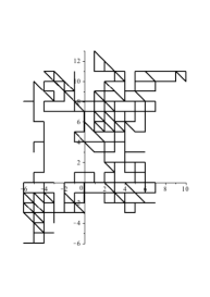
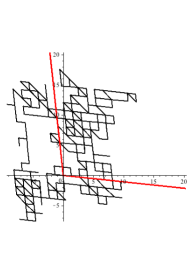
Figure 2. Five hundred steps with $\mathfrak{S}=\{(-1,0),(1,0),(0,-1),(0,1),(1,-1)\}$. Random walk $X$ with steps drawn uniformly from $\mathfrak{S}$ (left); random walk $Y$ with steps drawn from $\mathfrak{S}$ with probabilities $x_{0}^{i}y_{0}^{j}/\chi(x_{0},y_{0})$ (middle); random walk $Z$ obtained by decorrelating $Y$, with the cone $M(\mathbb{N}^{2})$ (right).

Drift and weights

The first step is to reduce to the case of a random walk $Y$ with no drift (i.e., $\mathbb{E}[(Y_{1}(k),Y_{2}(k))]=(0,0)$ for all $k$, where $Y_{1}$ and $Y_{2}$ are the coordinates of $Y$). This is achieved by giving different weights to each step: a weight $x_{0}>0$ to the East direction, $1/x_{0}$ to the West direction and simultaneously $y_{0}>0$ and $1/y_{0}$ to the North and South directions. Each step $(i,j)\in\mathfrak{S}$ is then given probability $x_{0}^{i}y_{0}^{j}/\chi(x_{0},y_{0})$. Finally, $x_{0}$ and $y_{0}$ are fixed by the condition $\mathbb{E}[(Y_{1}(k),Y_{2}(k))]=(0,0)$. (This is a special case of the Cramér transform, see [54].) By differentiation with respect to $x$ (resp. $y$), the expectations are obtained as

$$\mathbb{E}[Y_{1}(k)]=\frac{x_{0}}{\chi(x_{0},y_{0})}\frac{\partial\chi}{\partial x}(x_{0},y_{0}),\quad\mathbb{E}[Y_{2}(k)]=\frac{y_{0}}{\chi(x_{0},y_{0})}\frac{\partial\chi}{\partial y}(x_{0},y_{0}).$$

A correct choice of $(x_{0},y_{0})$ is therefore given by a positive solution to Eq. (2).

Since the step set of the walk is not confined to the right half-plane, the limit of $\chi(x,y)$ as $x\rightarrow 0+$ is infinite, similarly for $y\rightarrow 0+$ and for $x$ or $y$ tending to $+\infty$. This proves the existence of a solution. Its uniqueness comes from the convexity of $\chi$, a Laurent polynomial with positive coefficients.

This new random walk $Y$ is related to the original one: by induction on the number of steps,

$$\mathbb{P}\!\left[\sum_{k=1}^{n}(Y_{1}(k),Y_{2}(k))=(i,j),\,\tau>n\right]=x_{0}^{i}y_{0}^{j}\frac{|\mathfrak{S}|^{n}}{\chi(x_{0},y_{0})^{n}}\,\mathbb{P}\!\left[\sum_{k=1}^{n}(X_{1}(k),X_{2}(k))=(i,j),\,\tau>n\right],$$

where we use the same letter $\tau$ to denote the exit times of $X$ and $Y$ from $\mathbb{N}^{2}$. In view of Eq. (1), the number of walks can be read off the new walk as

$$f_{\mathfrak{S}}(i,j,n)=\frac{\rho(x_{0},y_{0})^{n}}{x_{0}^{i}y_{0}^{j}}\,\mathbb{P}\!\left[\sum_{k=1}^{n}(Y_{1}(k),Y_{2}(k))=(i,j),\,\tau>n\right].$$

Covariance and scaling

The second step is to reduce to the case of a random walk $Z$ with no drift and no correlation, i.e., whose covariance matrix $\operatorname{Cov}(Z)=(\mathbb{E}[Z_{i}Z_{j}])_{i,j}$ is the identity matrix.

The covariance matrix can be obtained from the characteristic polynomial again. Simple computations lead to

$$\operatorname{Cov}(Y)=\frac{1}{\chi(x_{0},y_{0})}\begin{pmatrix}x_{0}^{2}\frac{\partial^{2}\chi}{\partial x^{2}}(x_{0},y_{0})&x_{0}y_{0}\frac{\partial^{2}\chi}{\partial x\partial y}(x_{0},y_{0})\\ x_{0}y_{0}\frac{\partial^{2}\chi}{\partial x\partial y}(x_{0},y_{0})&y_{0}^{2}\frac{\partial^{2}\chi}{\partial y^{2}}(x_{0},y_{0})\end{pmatrix}.$$

One way to compute the appropriate scaling is in two steps. First, define a new walk obtained from $Y$ by $(W_{1},W_{2})=(Y_{1}/\sqrt{\mathbb{E}[Y_{1}^{2}]},Y_{2}/\sqrt{\mathbb{E}[Y_{2}^{2}]})$. By a direct computation, the walk $W$ has no drift and satisfies

$$\mathbb{E}[W_{1}^{2}]=\mathbb{E}[W_{2}^{2}]=1,\quad\mathbb{E}[W_{1}W_{2}]=\frac{\frac{\partial^{2}\chi}{\partial x\partial y}}{\sqrt{\frac{\partial^{2}\chi}{\partial x^{2}}\frac{\partial^{2}\chi}{\partial y^{2}}}}(x_{0},y_{0})=c.$$

By the Cauchy-Schwarz inequality, the correlation coefficient $c$ belongs to $[-1,1]$.

Finally, an uncorrelated walk is obtained by modifying the directions of the steps, defining a new walk $Z=MW$. We must have $\text{Cov}(Z)$ equal to the identity matrix. Since $\text{Cov}(Z)=M\text{Cov}(W)M^{\intercal}$ and since $\text{Cov}(W)$, as a covariance matrix, is symmetric positive-definite, we can find a diagonal matrix $D$ with positive diagonal entries and an orthonormal matrix $P$ such that $\text{Cov}(W)=PD{}P^{\intercal}$. The matrix $A=P{D}^{1/2}P^{\intercal}$ therefore satisfies $AA^{\intercal}=\text{Cov}(W)$, and the choice $M=A^{-1}=P{D}^{-1/2}P^{\intercal}$ is suitable.

In our case, we have

$$\text{Cov}(W)=\left(\begin{array}[]{cc}1&c\\ c&1\end{array}\right),\quad P=P^{\intercal}=P^{-1}=\frac{1}{\sqrt{2}}\left(\begin{array}[]{cr}1&1\\ 1&-1\end{array}\right),\quad D=\left(\begin{array}[]{cc}{1+c}&0\\ 0&{1-c}\end{array}\right).$$

We deduce that

$$M=A^{-1}=P{D}^{-1/2}P=\frac{1}{2\sqrt{1-c^{2}}}\left(\begin{array}[]{cc}\sqrt{1+c}+\sqrt{1-c}&\sqrt{1-c}-\sqrt{1+c}\\ \sqrt{1-c}-\sqrt{1+c}&\sqrt{1+c}+\sqrt{1+c}\end{array}\right).$$

Choosing $c=\sin(2\phi)$ and using easy trigonometric identities, we conclude that

$$M=\frac{1}{\sqrt{1-c^{2}}}\left(\begin{array}[]{cr}\cos(\phi)&-\sin(\phi)\\ -\sin(\phi)&\cos(\phi)\end{array}\right).$$

Now, the excursions of these walks are related by

$$\mathbb{P}\!\left[\sum_{k=1}^{n}(Y_{1}(k),Y_{2}(k))=(0,0),\,\tau>n\right] =\mathbb{P}\!\left[\sum_{k=1}^{n}(W_{1}(k),W_{2}(k))=(0,0),\,\tau>n\right],$$

$$=\mathbb{P}\!\left[\sum_{k=1}^{n}(Z_{1}(k),Z_{2}(k))=(0,0),\,\tau>n\right],$$

where the same letter $\tau$ is used to denote the first exit times, first for the walk $Y$ from $\mathbb{N}^{2}$, next for the walk $W$ from $\mathbb{N}^{2}$ and finally for the walk $Z$ from the cone $M(\mathbb{N}^{2})$, whose opening is $\arccos(-\sin 2\phi)=\arccos(-c).$ (See Figure 2.)

Asymptotic behavior of exit times

In these conditions, the result of Denisov and Wachtel [30, Theorem 6] proves in great generality that the exit time behaves like the exit time of the Brownian motion from that same cone. This is a classical topic of probability theory, in arbitrary dimension [1]. We content ourselves with sketching how the exponent $\pi/\arccos(-c)$ comes into play and refer to the literature for details. Our description follows closely that of DeBlassie [55] and Bañuelos and Smits [56] that we make explicit in our special case.

The probability $g(x,y,t)=\mathbb{P}_{(x,y)}[\tau\geq t]$ that a Brownian motion starting at $(x,y)$ inside the cone is still inside the cone at time $t$ obeys a diffusion equation

$$\left(\frac{\partial}{\partial t}-\frac{1}{2}\Delta\right)g(x,y,t)=0,$$

where $\Delta$ denotes the Laplacian, with $g(x,y,0)=1$ inside the cone and $g(x,y,t)=0$ for $t\geq 0$ on its border. Intuitively, this can be seen as the limit of the discrete recurrence for the probabilities of the random walk. It is then natural to pass to polar coordinates $(r,\theta)$. By a classical homogeneity property of the Brownian motion, the solution is actually a function of $t$ and $s=t/r^{2}$, which implies an extra equation $(\partial/{\partial t}+({r}/{2t})\partial/{\partial r})g(r,\theta,t)=0.$ Changing the variables into $u(s,\theta)=g(r,\theta,t)$ finally leads to

$$\left(L_{s}+\frac{\partial^{2}}{\partial\theta^{2}}\right)u(s,\theta)=0,\quad\text{where}\quad L_{s}=s^{2}\frac{\partial^{2}}{\partial s^{2}}+2(2s-1)\frac{\partial}{\partial s}$$

with boundary conditions $u(0,\theta)=1$ for $\theta$ inside the cone and $u(s,\theta)=0$ for $s\geq 0$ on its border. This problem is solved by the method of separation of variables: if a solution can be written $A(s)B(\theta)$, then $L_{s}(A(s))/A(s)=-B^{\prime\prime}(\theta)/B(\theta)$. The left-hand side depends only on $s$ and the right-hand side only on $\theta$ and thus they are both equal to a constant $\lambda$. In particular $B^{\prime\prime}(\theta)+\lambda B(\theta)=0$ with boundary conditions $B(0)=B(\arccos(-c))=0$ forces $\lambda$ to be of the form $\mu_{k}^{2}=(k\pi/\arccos(-c))^{2}$, $k\in\mathbb{N}\setminus\{0\}$ with corresponding solution $\sin(\theta\mu_{k})$. To each such $\lambda_{k}=\mu_{k}^{2}$ corresponds a solution of the left-hand side in terms of a hypergeometric series ${}_{1}F_{1}$ (see [57, §16.11]), namely

$$A_{k}(s)=(2s)^{-\mu_{k}/2}{}_{1}F_{1}\left(\mu_{k}/2,\mu_{k}+1,-1/(2s)\right),\quad\text{with}\quad\lim_{s\rightarrow 0+}A_{k}(s)=\frac{2^{\mu_{k}}}{\sqrt{\pi}}\Gamma\!\left(\frac{\mu_{k}+1}{2}\right).$$

By completeness of the set of eigenfunctions (or Fourier expansion in that case), the solution of the diffusion equation therefore writes as a linear combination

$$g(r,\theta,t)=\sum{c_{k}\sin(\mu_{k}\theta)A_{k}(t/r^{2})}.$$

The coefficients $c_{k}$ are then given by the Fourier expansion of the boundary condition $u(0,\theta)=1$. Thus, finally, the desired probability $g(x,y,t)$ has leading term in $t^{-\mu_{1}/2}=t^{-\pi/(2\arccos(-c))}$ as $t\rightarrow\infty$. The relation to the discrete random walk due to Denisov and Wachtel then gives

$$\mathbb{P}_{(x,y)}[\tau\geq n]\sim\kappa n^{-\pi/(2\arccos(-c))},$$

for some constant $\kappa$ depending on $x$ and $y$.

Local limit theorem

The conclusion is now explicitly in Denisov and Wachtel [30, Theorem 6 and Lemma 13].

Periodic step sets

An examination of the different cases of periodic step sets (they are marked with a star in Tables 4 and 4) shows that the period is necessarily $2$. In particular, we have $e_{2n+1}=0$ for all $n\geq 0$. However, a reduction to the previous case is obtained by changing the step set into $\mathfrak{S}+\mathfrak{S}$ and $n$ into $n/2$. ∎

2.4. Algorithmic irrationality proof

Let $\mathfrak{S}\subseteq\{0,\pm 1\}^{2}$ be one of the 51 nonsingular step sets with infinite group (see Table 4 in Appendix 4). By Theorem 4, the singular exponent $\alpha$ in the asymptotic expansion of the excursion sequence $(e^{\mathfrak{S}}_{n})_{n\geq 0}$ is equal to $-1-\pi/\arccos(-c)$, where $c$ is an algebraic number. Therefore, if $\arccos(c)/\pi$ is an irrational number, then by Theorem 3, the generating function $F_{\mathfrak{S}}(0,0,t)$ is not D-finite.

We now explain how, starting from the step set $\mathfrak{S}$ one can algorithmically prove that $\arccos(c)/\pi$ is irrational. This effective proof decomposes into two main steps, solved by two different algorithms. The first algorithm computes the minimal polynomial $\mu_{c}(t)\in\mathbb{Q}[t]$ of $c$ starting from $\mathfrak{S}$. The second one performs computations on $\mu_{c}(t)$ showing that $\arccos(c)/\pi$ is irrational.

2.4.1. Computing the minimal polynomial of the correlation coefficient

Given $\chi=\chi_{\mathfrak{S}}$ the characteristic polynomial of the step set $\mathfrak{S}$, Theorem 4 shows that the exponential growth $\rho$ and the correlation coefficient $c$ are algebraic numbers, for which equations can be obtained by eliminating $x$ and $y$ from the algebraic equations

$$\frac{\partial\chi}{\partial x}=0,\qquad\frac{\partial\chi}{\partial y}=0,\qquad\rho-\chi=0,\qquad c^{2}-\frac{\left({\frac{\partial^{2}\chi}{\partial x\partial y}}\right)^{2}}{\frac{\partial^{2}\chi}{\partial x^{2}}\cdot\frac{\partial^{2}\chi}{\partial y^{2}}}=0.$$

This elimination is a routine task in effective algebraic geometry, usually performed with Gröbner bases for lexicographic or elimination orders [58]. Let $\chi_{x}$ and $\chi_{y}$ denote respectively the numerators of $\frac{\partial\chi}{\partial x}$ and of $\frac{\partial\chi}{\partial y}$. The solutions of $\chi_{x}=\chi_{y}=0$ contain the solutions of $\frac{\partial\chi}{\partial x}=\frac{\partial\chi}{\partial y}=0$, but may also contain spurious solutions at $x=0$ or $y=0$ provoked by the multiplication by powers of $x$ and $y$. These are removed by introducing a new variable $u$ and considering the zero-dimensional ideal $I$ of $\mathbb{Q}[x,y,u]$ generated by $(\chi_{x},\chi_{y},1-uxy)$.

For any zero $(x_{0},y_{0})$ of the system $\chi_{x}(x_{0},y_{0})=\chi_{y}(x_{0},y_{0})=0$ and any polynomials $P(x,y)$ and $Q(x,y)$ such that $Q\not\in I$, the algebraic number $P(x_{0},y_{0})/Q(x_{0},y_{0})$ is a root of a generator of the ideal $I+\langle P(x,y)-tQ(x,y)\rangle\cap\mathbb{Q}[t]$. This can be used to compute annihilating polynomials for $\rho$ and $c$.

This computation is summarized in the following algorithm.

• A step set $\mathfrak{S}$ satisfying the assumptions of Theorem 4

• The minimal polynomials of $\rho$ and $c$ defined in Theorem 4

• Set $\chi(x,y):=\sum_{(i,j)\in\mathfrak{S}}x^{i}y^{j}$, and compute $\chi_{x}:=\textsf{numer}(\frac{\partial\chi}{\partial x})$, $\chi_{y}:=\textsf{numer}(\frac{\partial\chi}{\partial y})$.

• Compute the Gröbner basis of the ideal generated in $\mathbb{Q}[x,y,t,u]$ by $(\chi_{x},\chi_{y},\textsf{numer}(t-\chi),1-uxy)$ for a term order that eliminates $x,y$ and $u$. Isolate the unique polynomial in this basis that depends only on $t$, factor it, and identify its factor $\mu_{\rho}$ that annihilates $\rho$.

• Compute the polynomial

  $$P(x,y,t):=\textsf{numer}\left(t^{2}-\frac{\left({\frac{\partial^{2}\chi}{\partial x\partial y}}\right)^{2}}{{\frac{\partial^{2}\chi}{\partial x^{2}}\cdot\frac{\partial^{2}\chi}{\partial y^{2}}}}\right)$$

  and eliminate $x,y$ and $u$ by computing a Gröbner basis of the ideal generated in $\mathbb{Q}[x,y,t,u]$ by $(\chi_{x},\chi_{y},P,1-uxy)$ for a term order that eliminates $x,y$ and $u$. Isolate the unique polynomial in this basis that depends only on $t$, factor it, and identify its factor $\mu_{c}$ that annihilates $c$.

The identification of the proper factor is achieved for instance by computing a rough approximation of the numerical values of $\rho$ and $c$ using Eq. (3) and comparing with the numerical roots of the factors. If needed, the numerical values can then be refined to arbitrary precision using the correct factor.

Table 4 in Appendix 4 displays the minimal polynomials of $\rho$ and of $c$ obtained using this algorithm.

2.4.2. Proving that the arccosine of the correlation coefficient is not commensurable with $\pi$

Given the minimal polynomial $\mu_{c}$ of the correlation coefficient $c$, we now want to check that $\arccos(c)/\pi$ is irrational. General classification results exist, e.g., [59], but they are not sufficient for our purpose. Instead, we rather prove that $\arccos(c)/\pi$ is irrational in an algorithmic way. This is based on the observation that if $\arccos(c)/\pi$ were rational, then $c$ would be of the form $(z+1/z)/2=(z^{2}+1)/(2z)$ with $z$ a root of unity. This implies that the numerator of the rational function $\mu_{c}(\frac{x^{2}+1}{2x})$ would possess a root which is a root of unity. In other words, the polynomial $R(x)=x^{\operatorname{deg}\mu_{c}}\mu_{c}(\frac{x^{2}+1}{2x})$ would be divisible by a cyclotomic polynomial. This possibility can be discarded by analyzing the minimal polynomials $\mu_{c}$ displayed in Table 4 in Appendix 4.

Indeed, in all the 51 cases, the polynomial $R(x)$ is irreducible and has degree $2\operatorname{deg}(\mu_{c})$, thus at most 28. Now, it is known that if the cyclotomic polynomial $\Phi_{N}$ has degree at most 30, then $N$ is at most 150 [60, Theorem 15], and the coefficients of $\Phi_{N}$ belong to the set $\{-2,-1,0,1,2\}$ [61]. Computing $R$ in the 51 cases shows that it has at least one coefficient of absolute value at least 3. This allows to conclude that $R$ is not a cyclotomic polynomial, and therefore that $\arccos(c)/\pi$ is irrational, and finishes the proof of Theorem 1.

2.5. Example

We now illustrate the systematic nature of our algorithms on Example 23 of Table 4, i.e., walks with step set $\mathfrak{S}=\{(-1,0),(0,1),(1,0),(1,-1),(0,-1)\}$. For ease of use, we give explicit Maple instructions.

Step 1

The characteristic polynomial of the step set is

S:=[[-1,0],[0,1],[1,0],[1,-1],[0,-1]]:
chi:=add(x^s[1]*y^s[2],s=S);

$$\chi:=\frac{1}{x}+\frac{1}{y}+x+y+\frac{x}{y},$$

whose derivatives have numerators

chi_x:=numer(diff(chi,x));chi_y:=numer(diff(chi,y));

(4) $$\chi_{x}:=x^{2}+x^{2}y-y,\qquad\chi_{y}:=y^{2}-x-1.$$

These define the system (2).

Step 2

We now compute a polynomial that vanishes at $\rho=\chi(x_{0},y_{0})$ when $(x_{0},y_{0})$ is a solution of (4). To this aim, we eliminate $x$, $y$ and $u$ in $\{\chi_{x},\chi_{y},\textsf{numer}(\chi)-t\textsf{denom}(\chi),1-uxy\}$ by a Gröbner basis computation using an elimination order with $(x,y,u)>t$. In Maple, this is provided by the command

G:=Groebner[Basis]([chi_x,chi_y,numer(t-chi),1-u*x*y],lexdeg([x,y,u],[t])):

which returns five polynomials, only one of which is free of $x$ and $y$, namely

p:=factor(op(remove(has,G,{x,y,u})));

$$p:=(t+1)(t^{3}+t^{2}-18t-43).$$

In this case, since we know that $\rho>0$, we do not need to compute a numerical approximation of it using Eq. (3), but identify its minimal polynomial directly as $\mu_{\rho}=t^{3}+t^{2}-18t-43$, which gives the entry in Column 3 of Table 4. The numerical value for $\rho$ in Table 4 is given by

fsolve(p,t,0..infinity);

$$4.729031538.$$

Note that in this example, the introduction of the variable $u$ and the polynomial $1-uxy$ are unnecessary since neither $x=0$ nor $y=0$ are solutions of $\chi_{x}=\chi_{y}=0$.

Step 3

Next, we obtain a polynomial which vanishes at $c$ by a very similar computation:

G:=Groebner[Basis]([numer(t^2-diff(chi,x,y)^2/diff(chi,x,x)/diff(chi,y,y)),
                 chi_x,chi_y,1-x*y*u],lexdeg([x,y,u],[t]));

Again, this command returns five polynomials, with one of them free of $x$ and $y$, namely

p:=factor(op(remove(has,G,{x,y,u})));

$$p:=(4t^{2}+1)(8t^{3}+8t^{2}+6t+1)(8t^{3}-8t^{2}+6t-1).$$

This polynomial has only two real roots, $\pm c$. Since $c<0$ (to see this, it suffices to use the expression (3) of $c$), we identify its minimal polynomial as $\mu_{c}=8t^{3}+8t^{2}+6t+1$, which gives the entry in Column 4 of Table 4. Again, the numerical value for $\alpha$ in Table 4 is given by

mu_c:=8*t^3+8*t^2+6*t+1:
evalf(-1-Pi/arccos(-fsolve(mu_c,t)));

$$-3.320191962.$$

Step 4.

To conclude, we compute the polynomial

$$R(x)=x^{3}\mu_{c}\left(\frac{x^{2}+1}{2x}\right)=x^{6}+2x^{5}+6x^{4}+5x^{3}+6x^{2}+2x+1.$$

This polynomial does not have any root that is a root of unity, since it is irreducible and not cyclotomic:

R:=numer(subs(t=(x^2+1)/x/2, mu_c));Ψ
irreduc(R),numtheory[iscyclotomic](R,x);

$$\text{\em true},\text{\em false}$$

This completes the proof that the generating function for this walk is not D-finite.

3. Conclusion

3.1. Extensions

The result of Denisov and Wachtel that is the basis of our work holds in arbitrary dimension and for walks with steps of arbitrary length. The consequence that we state (Theorem 4) is actually not restricted to small step walks. Preliminary experiments indicate that it serves as a very efficient filter in a quest for holonomic excursion sequences.

In higher dimension, Theorem 4 no longer holds. The results of Denisov and Wachtel lead to a similar statement involving the first eigenvalue of a Laplacian on a spherical domain, which is difficult to estimate, not to mention irrationality proofs.

On the other hand, the arithmetic result of Theorem 3 has a much wider scope of application in proving non-D-finiteness of combinatorial sequences and deserves to be better known.

3.2. Open problems

Since our approach brings together a strong arithmetic result (Theorem 3) and a strong probabilistic result (Theorem 4), it appears natural to search for alternative simpler proofs of these results.

Proving that $\alpha$ is transcendental

In Section 2.4, we are able to prove that for the 51 nonsingular models, the exponent $\alpha$ in the asymptotic expansion of the excursion sequence is irrational. It is worth mentioning that if it were possible to prove that $\alpha$ is not only irrational, but also transcendental, then Theorem 3 would not be needed.

Simpler proof of Theorem 3

The current proof of Theorem 3 is based on several strong results from arithmetic theory [52, 48, 53, 44]. It would be interesting to know whether Theorem 3 admits a simpler, direct proof.

Combinatorial proof of Theorem 4

Theorem 4 relies on properties of the Brownian motion that are inherently continuous. Finding a purely combinatorial proof, e.g., with generating functions, would shed interesting light on this problem.

Total number of walks

Our work deals with the nature of the full generating function $F_{\mathfrak{S}}(x,y,t)$ and its specialization at $(x,y)=(0,0)$. The actual nature of $F_{\mathfrak{S}}(1,1,t)$ is still partly unknown at this stage, although the conjectural classification in [23, 43] suggests that $F_{\mathfrak{S}}(1,1,t)$ is not-D-finite in all 51 non-singular cases with infinite group. Another approach might be needed in this problem. Indeed, when $\mathfrak{S}=\{(1,0),(0,1),(1,1),(-1,-1)\}$, the total number of walks of length $n$ seems to behave like $c\cdot 4^{n}$, but the generating function itself seems to be non-D-finite.

Acknowledgements. We wish to thank Tanguy Rivoal, Denis Denisov and Vitali Wachtel for stimulating exchanges. We also thank the referees for their comments. Work of the first and the third authors was supported in part by the Microsoft Research-Inria Joint Centre.

4. Appendix

Table 1 The 51 nonsingular step sets in the quarter plane with an infinite group, and the asymptotics of their excursions (valid for even $n$ in the periodic cases). The numbering used in column “Tag” corresponds to the order of the step sets in Table 4 of [28]. Periodic walks have tags marked with a star.

Tag	Steps	First terms	Asymptotics	Tag	Steps	First terms	Asymptotics
3		1, 0, 1, 2, 2, 13, 21, 67, 231	$\dfrac{3.799605^{n}}{n^{2.610604}}$	4		1, 0, 0, 2, 2, 0, 16, 44, 28	$\dfrac{3.608079^{n}}{n^{2.720448}}$
5		1, 0, 1, 2, 2, 14, 21, 76, 252	$\dfrac{3.799605^{n}}{n^{2.318862}}$	6		1, 0, 1, 2, 2, 13, 21, 67, 231	$\dfrac{3.799605^{n}}{n^{2.610604}}$
7⋆		1, 0, 1, 0, 4, 0, 29, 0, 230	$\dfrac{3.800378^{n}}{n^{2.521116}}$	8		1, 0, 1, 1, 2, 7, 10, 38, 89	$\dfrac{3.799605^{n}}{n^{3.637724}}$
9		1, 0, 1, 1, 2, 7, 10, 38, 89	$\dfrac{3.799605^{n}}{n^{3.637724}}$	10		1, 0, 0, 1, 2, 0, 5, 26, 28	$\dfrac{3.608079^{n}}{n^{3.388025}}$
11⋆		1, 0, 0, 0, 2, 0, 6, 0, 42	$\dfrac{3.800378^{n}}{n^{3.918957}}$	12		1, 0, 0, 1, 0, 1, 5, 1, 18	$\dfrac{3.799605^{n}}{n^{5.136154}}$
14		1, 0, 0, 1, 2, 0, 5, 26, 28	$\dfrac{3.608079^{n}}{n^{3.388025}}$	16		1, 0, 1, 2, 2, 14, 21, 76, 252	$\dfrac{3.799605^{n}}{n^{2.318862}}$
17⋆		1, 0, 1, 0, 4, 0, 29, 0, 230	$\dfrac{3.800378^{n}}{n^{2.521116}}$	18		1, 0, 0, 2, 2, 0, 16, 44, 28	$\dfrac{3.608079^{n}}{n^{2.720448}}$
19⋆		1, 0, 0, 0, 2, 0, 6, 0, 42	$\dfrac{3.800378^{n}}{n^{3.918957}}$	20		1, 0, 1, 2, 4, 14, 45, 120, 468	$\dfrac{4.372923^{n}}{n^{2.482876}}$
21		1, 0, 1, 1, 4, 7, 25, 64, 201	$\dfrac{4.214757^{n}}{n^{3.347502}}$	23		1, 0, 2, 1, 10, 14, 75, 178, 738	$\dfrac{4.729032^{n}}{n^{3.320192}}$
24		1, 0, 2, 2, 10, 26, 86, 312, 1022	$\dfrac{4.729032^{n}}{n^{2.757466}}$	25		1, 0, 2, 2, 11, 27, 101, 348, 1237	$\dfrac{4.729032^{n}}{n^{2.397625}}$
26		1, 0, 2, 2, 11, 27, 101, 348, 1237	$\dfrac{4.729032^{n}}{n^{2.397625}}$	27⋆		1, 0, 2, 0, 13, 0, 124, 0, 1427	$\dfrac{4.569086^{n}}{n^{2.503534}}$
28		1, 0, 1, 2, 4, 13, 36, 111, 343	$\dfrac{4.214757^{n}}{n^{2.742114}}$	29⋆		1, 0, 1, 0, 5, 0, 35, 0, 313	$\dfrac{4.569086^{n}}{n^{3.985964}}$
30		1, 0, 1, 1, 6, 17, 58, 202, 749	$\dfrac{5^{n}}{n^{2.722859}}$	31		1, 0, 0, 1, 2, 1, 11, 27, 60	$\dfrac{4.372923^{n}}{n^{4.070925}}$
32⋆		1, 0, 2, 0, 13, 0, 124, 0, 1427	$\dfrac{4.569086^{n}}{n^{2.503534}}$	33		1, 0, 1, 1, 4, 7, 25, 64, 201	$\dfrac{4.214757^{n}}{n^{3.347502}}$
34⋆		1, 0, 1, 0, 5, 0, 35, 0, 313	$\dfrac{4.569086^{n}}{n^{3.985964}}$	35		1, 0, 1, 1, 3, 8, 19, 65, 177	$\dfrac{4.729032^{n}}{n^{4.514931}}$
36		1, 0, 0, 1, 2, 1, 11, 27, 60	$\dfrac{4.372923^{n}}{n^{4.070925}}$	37		1, 0, 1, 2, 4, 13, 36, 111, 343	$\dfrac{4.214757^{n}}{n^{2.742114}}$
38		1, 0, 2, 2, 10, 26, 86, 312, 1022	$\dfrac{4.729032^{n}}{n^{2.757466}}$	39		1, 0, 1, 1, 3, 8, 19, 65, 177	$\dfrac{4.729032^{n}}{n^{4.514931}}$
40		1, 0, 0, 2, 4, 8, 28, 108, 372	$\dfrac{5^{n}}{n^{3.383396}}$	41		1, 0, 1, 2, 4, 14, 45, 120, 468	$\dfrac{4.372923^{n}}{n^{2.482876}}$
42		1, 0, 0, 2, 4, 8, 28, 108, 372	$\dfrac{5^{n}}{n^{3.383396}}$	43		1, 0, 2, 2, 13, 27, 140, 392, 1882	$\dfrac{5.064419^{n}}{n^{2.491053}}$
44		1, 0, 2, 3, 15, 51, 208, 893, 3841	$\dfrac{5.891838^{n}}{n^{2.679783}}$	45		1, 0, 1, 1, 5, 8, 40, 91, 406	$\dfrac{5.064419^{n}}{n^{4.036441}}$
46		1, 0, 1, 2, 8, 22, 101, 364, 1618	$\dfrac{5.799605^{n}}{n^{2.959600}}$	47		1, 0, 1, 3, 7, 29, 101, 404, 1657	$\dfrac{5.891838^{n}}{n^{3.471058}}$
48		1, 0, 1, 1, 5, 8, 40, 91, 406	$\dfrac{5.064419^{n}}{n^{4.036441}}$	49		1, 0, 2, 2, 13, 27, 140, 392, 1882	$\dfrac{5.064419^{n}}{n^{2.491053}}$
50		1, 0, 2, 3, 15, 51, 208, 893, 3841	$\dfrac{5.891838^{n}}{n^{2.679783}}$	51		1, 0, 1, 3, 7, 29, 101, 404, 1657	$\dfrac{5.891838^{n}}{n^{3.471058}}$
52		1, 0, 1, 1, 8, 18, 90, 301, 1413	$\dfrac{5.799605^{n}}{n^{3.042101}}$	53		1, 0, 1, 2, 8, 22, 101, 364, 1618	$\dfrac{5.799605^{n}}{n^{2.959600}}$
54		1, 0, 3, 5, 30, 111, 548, 2586, 13087	$\dfrac{6.729032^{n}}{n^{2.667986}}$	55		1, 0, 2, 4, 16, 64, 266, 1210, 5630	$\dfrac{6.729032^{n}}{n^{3.497037}}$
56		1, 0, 2, 4, 16, 64, 266, 1210, 5630	$\dfrac{6.729032^{n}}{n^{3.497037}}$

Table 2 Minimal polynomials of the growth constants $\rho$ and of the correlation coefficients $c$ for the 51 nonsingular walks in the quarter plane with an infinite group. Each blank entry in the table coincides with the first non-empty entry above it.

Tag	Steps	Minimal polynomial $\mu_{\rho}$ of $\rho$	Minimal polynomial $\mu_{c}$ of $c=-\cos(\frac{\pi}{1+\alpha})$
12		$t^{4}+t^{3}-8t^{2}-36t-11$	$t^{4}+\frac{9}{2}t^{3}+\frac{27}{4}t^{2}+\frac{35}{8}t+\frac{17}{16}$
5, 16	,		$t^{4}-\frac{9}{2}t^{3}+\frac{27}{4}t^{2}-\frac{35}{8}t+\frac{17}{16}$
3, 6	,		$t^{8}+\frac{1}{4}t^{6}-\frac{3}{16}t^{4}+\frac{3}{64}t^{2}-\frac{1}{256}$
8, 9	,
7⋆, 17⋆	,	$t^{6}-11t^{4}-32t^{2}-256$	$t^{6}+\frac{3}{4}t^{4}+2t^{2}-\frac{1}{2}$
11⋆, 19⋆	,
4, 18	,	$t^{5}+t^{4}+t^{3}-30t^{2}-96t-91$	$t^{10}+2t^{8}+t^{6}-\frac{1}{64}t^{4}+\frac{3}{256}t^{2}-\frac{1}{1024}$
10, 14	,
20, 41	,	$t^{5}-2t^{4}-4t^{3}-31t^{2}+23t-41$	$t^{10}+t^{8}+\frac{157}{32}t^{6}+\frac{145}{128}t^{4}+\frac{1681}{512}t^{2}-\frac{2209}{2048}$
31, 36	,
21, 33	,	$t^{5}+2t^{4}-7t^{3}-46t^{2}-116t-131$	$t^{10}+\frac{3}{2}t^{8}+\frac{13}{16}t^{6}+\frac{5}{64}t^{4}+\frac{3}{256}t^{2}-\frac{1}{1024}$
28, 37	,
23		$t^{3}+t^{2}-18t-43$	$t^{3}+t^{2}+\frac{3}{4}t+\frac{1}{8}$
24, 38	,		$t^{3}-t^{2}+\frac{3}{4}t-\frac{1}{8}$
25, 26	,		$t^{6}-t^{4}+\frac{7}{16}t^{2}-\frac{5}{64}$
35, 39	,
27⋆, 32⋆	,	$t^{6}-20t^{4}-16t^{2}-48$	$t^{6}+2t^{4}+\frac{5}{2}t^{2}-\frac{3}{4}$
29⋆, 34⋆	,
30		$t-5$	$t-\frac{1}{4}$
40, 42	,		$t+\frac{1}{4}$
43, 49	,	$t^{6}+2t^{5}-18t^{4}-67t^{3}-108t^{2}-40t-19$	$t^{12}+\frac{11}{4}t^{10}+\frac{107}{16}t^{8}+\frac{145}{32}t^{6}+\frac{455}{128}t^{4}-\frac{2859}{1024}t^{2}+\frac{1521}{4096}$
45, 48	,
44, 50	,	$t^{7}+3t^{6}-18t^{5}-127t^{4}-328t^{3}-560t^{2}-704t-448$	$t^{14}+\frac{23}{4}t^{12}+\frac{25}{2}t^{10}+\frac{971}{64}t^{8}+\frac{421}{32}t^{6}+\frac{307}{64}t^{4}+\frac{107}{64}t^{2}-\frac{49}{256}$
47, 51	,
52		$t^{4}-7t^{3}+10t^{2}-24t+37$	$t^{4}+\frac{1}{2}t^{3}+\frac{55}{4}t^{2}+\frac{19}{8}t+\frac{1}{16}$
46, 53	,		$t^{4}-\frac{1}{2}t^{3}+\frac{55}{4}t^{2}-\frac{19}{8}t+\frac{1}{16}$
54		$t^{3}-5t^{2}-10t-11$	$t^{3}+\frac{11}{4}t-\frac{7}{8}$
55, 56	,		$t^{3}+\frac{11}{4}t+\frac{7}{8}$

References

- [1] Frank Spitzer. Principles of random walk. The University Series in Higher Mathematics. D. Van Nostrand Co., Inc., Princeton, N.J.-Toronto-London, 1964.
- [2] William Feller. An introduction to probability theory and its applications. Vol. I. Third edition. John Wiley & Sons Inc., New York, 1968.
- [3] Peter G. Doyle and J. Laurie Snell. Random walks and electric networks, volume 22 of Carus Mathematical Monographs. Mathematical Association of America, Washington, DC, 1984.
- [4] J. W. Cohen. Analysis of random walks, volume 2 of Studies in Probability, Optimization and Statistics. IOS Press, Amsterdam, 1992.
- [5] Roberto Fernández, Jürg Fröhlich, and Alan D. Sokal. Random walks, critical phenomena, and triviality in quantum field theory. Texts and Monographs in Physics. Springer-Verlag, Berlin, 1992.
- [6] George H. Weiss. Aspects and applications of the random walk. Random Materials and Processes. North-Holland Publishing Co., Amsterdam, 1994.
- [7] Wolfgang Woess. Random walks on infinite graphs and groups, volume 138 of Cambridge Tracts in Mathematics. Cambridge University Press, Cambridge, 2000.
- [8] A. A. Borovkov and K. A. Borovkov. Asymptotic analysis of random walks, volume 118 of Encyclopedia of Mathematics and its Applications. Cambridge University Press, Cambridge, 2008. Heavy-tailed distributions, Translated from the Russian by O. B. Borovkova.
- [9] Gregory F. Lawler and Vlada Limic. Random walk: a modern introduction, volume 123 of Cambridge Studies in Advanced Mathematics. Cambridge University Press, Cambridge, 2010.
- [10] Philippe Blanchard and Dimitri Volchenkov. Random walks and diffusions on graphs and databases. Springer Series in Synergetics. Springer, Heidelberg, 2011. An introduction.
- [11] Georg Pólya. Über eine Aufgabe der Wahrscheinlichkeitsrechnung betreffend die Irrfahrt im Straßennetz. Math. Ann., 84(1-2):149–160, 1921.
- [12] T. V. Narayana. Lattice path combinatorics with statistical applications, volume 23 of Mathematical Expositions. University of Toronto Press, Toronto, Ont., 1979.
- [13] Sri Gopal Mohanty. Lattice path counting and applications. Academic Press [Harcourt Brace Jovanovich Publishers], New York, 1979. Probability and Mathematical Statistics.
- [14] G. Kreweras. Sur une classe de problèmes de dénombrement liés au treillis des partitions des entiers. Cahiers du B.U.R.O., 6:5–105, 1965.
- [15] Mary Anne Maher. Random walks on the positive quadrant. ProQuest LLC, Ann Arbor, MI, 1978. Thesis (Ph.D.)–University of Rochester.
- [16] Dominique Gouyou-Beauchamps. Chemins sous-diagonaux et tableaux de Young. In Combinatoire énumérative (Montreal, Que., 1985/Quebec, Que., 1985), volume 1234 of Lecture Notes in Math., pages 112–125. Springer, Berlin, 1986.
- [17] Ira M. Gessel and Doron Zeilberger. Random walk in a Weyl chamber. Proc. Amer. Math. Soc., 115(1):27–31, 1992.
- [18] Guy Fayolle, Roudolf Iasnogorodski, and Vadim Malyshev. Random walks in the quarter-plane, volume 40 of Applications of Mathematics (New York). Springer-Verlag, Berlin, 1999. Algebraic methods, boundary value problems and applications.
- [19] Mireille Bousquet-Mélou. Counting walks in the quarter plane. In Mathematics and computer science, II (Versailles, 2002), Trends Math., pages 49–67. Birkhäuser, Basel, 2002.
- [20] M. Bousquet-Mélou and M. Petkovšek. Walks confined in a quadrant are not always D-finite. Theoret. Comput. Sci., 307(2):257–276, 2003.
- [21] M. Bousquet-Mélou. Walks in the quarter plane: Kreweras’ algebraic model. Ann. Appl. Probab., 15(2):1451–1491, 2005.
- [22] M. Mishna. Classifying lattice walks in the quarter plane. In Proceedings of FPSAC’07, Tianjin, China, 2007. Available on-line at http://arxiv.org/abs/math/0611651.
- [23] Alin Bostan and Manuel Kauers. Automatic classification of restricted lattice walks. In DMTCS Proceedings of the 21st International Conference on Formal Power Series and Algebraic Combinatorics (FPSAC’09), Hagenberg, Austria, pages 203–217, 2009.
- [24] Manuel Kauers, Christoph Koutschan, and Doron Zeilberger. Proof of Ira Gessel’s lattice path conjecture. Proc. Natl. Acad. Sci. USA, 106(28):11502–11505, 2009.
- [25] Marni Mishna. Classifying lattice walks restricted to the quarter plane. J. Combin. Theory Ser. A, 116(2):460–477, 2009.
- [26] Marni Mishna and Andrew Rechnitzer. Two non-holonomic lattice walks in the quarter plane. Theoret. Comput. Sci., 410(38-40):3616–3630, 2009.
- [27] Alin Bostan and Manuel Kauers. The complete generating function for Gessel walks is algebraic. Proceedings of the American Mathematical Society, 138(9):3063–3078, September 2010. With an Appendix by Mark van Hoeij.
- [28] Mireille Bousquet-Mélou and Marni Mishna. Walks with small steps in the quarter plane. In Algorithmic probability and combinatorics, volume 520 of Contemp. Math., pages 1–39. Amer. Math. Soc., Providence, RI, 2010.
- [29] G. Fayolle and K. Raschel. On the holonomy or algebraicity of generating functions counting lattice walks in the quarter-plane. Markov Process. Related Fields, 16(3):485–496, 2010.
- [30] Denis Denisov and Vitali Wachtel. Random walks in cones. Annals of Probability, 2013. To appear.
- [31] G. Fayolle and K. Raschel. Random walks in the quarter plane with zero drift: an explicit criterion for the finiteness of the associated group. Markov Process. Related Fields, 17(4):619–636, 2011.
- [32] Irina Kurkova and Kilian Raschel. Explicit expression for the generating function counting Gessel’s walks. Adv. in Appl. Math., 47(3):414–433, 2011.
- [33] Irina Kurkova and Kilian Raschel. On the functions counting walks with small steps in the quarter plane. Publ. Math. Inst. Hautes Études Sci., 116(1):69–114, 2012.
- [34] Guy Fayolle and Kilian Raschel. Some exact asymptotics in the counting of walks in the quarter plane. In 23rd Intern. Meeting on Probabilistic, Combinatorial, and Asymptotic Methods for the Analysis of Algorithms (AofA’12), Discrete Math. Theor. Comput. Sci. Proc., AQ, pages 109–124. Assoc. Discrete Math. Theor. Comput. Sci., Nancy, 2012.
- [35] K. Raschel. Counting walks in a quadrant: a unified approach via boundary value problems. J. Eur. Math. Soc. (JEMS), 14(3):749–777, 2012.
- [36] S. Melczer and M. Mishna. Singularity analysis via the iterated kernel method. In DMTCS Proceedings of FPSAC’13, Paris, France, pages 481–492, 2013.
- [37] A. Bostan, F. Chyzak, M. van Hoeij, M. Kauers, and L. Pech. Explicit differentiably finite generating functions of walks with small steps in the quarter plane. In preparation (2013).
- [38] Alin Bostan, Irina Kurkova, and Kilian Raschel. A human proof of Gessel’s lattice path conjecture. Technical Report 1309.1023, arXiv, 2013. Available on-line at http://arxiv.org/abs/1309.1023.
- [39] Samuel Johnson, Marni Mishna, and Karen Yeats. Towards a combinatorial understanding of lattice path asymptotics. Technical Report 1305.7418, arXiv, 2013. Available on-line at http://arxiv.org/abs/math/1304.7418.
- [40] L. Lipshitz. -finite power series. Journal of Algebra, 122(2):353–373, 1989.
- [41] Philippe Flajolet and Robert Sedgewick. Analytic combinatorics. Cambridge University Press, Cambridge, 2009.
- [42] C. Banderier and P. Flajolet. Basic analytic combinatorics of directed lattice paths. Theoret. Comput. Sci., 281(1-2):37–80, 2002.
- [43] Alin Bostan and Manuel Kauers. Unpublished notes, 2008.
- [44] B. Dwork, G. Gerotto, and F. J. Sullivan. An introduction to -functions, volume 133 of Annals of Mathematics Studies. Princeton University Press, Princeton, NJ, 1994.
- [45] Yves André. Séries Gevrey de type arithmétique. I. Théorèmes de pureté et de dualité. Ann. of Math. (2), 151(2):705–740, 2000.
- [46] S. Garoufalidis. -functions and multisum versus holonomic sequences. Advances in Mathematics, 220(6):1945–1955, 2009.
- [47] Philippe Flajolet. Analytic models and ambiguity of context-free languages. Theoret. Comput. Sci., 49(2-3):283–309, 1987. Twelfth international colloquium on automata, languages and programming (Nafplion, 1985).
- [48] Yves André. -functions and geometry. Aspects of Mathematics, E13. Friedr. Vieweg & Sohn, Braunschweig, 1989.
- [49] Carl Ludwig Siegel. Über einige Anwendungen Diophantischer Approximationen. Abh. Pruess. Akad. Wiss. Phys. Math. Kl., 1:41–69, 1929.
- [50] G. D. Birkhoff and W. J. Trjitzinsky. Analytic theory of singular difference equations. Acta Mathematica, 60:1–89, 1932.
- [51] H. L. Turrittin. Convergent solutions of ordinary linear homogeneous differential equations in the neighbourhood of an irregular singular point. Acta. Math., 93:27–66, 1955.
- [52] D. V. Chudnovsky and G. V. Chudnovsky. Applications of Padé approximations to Diophantine inequalities in values of -functions. In Number theory (New York, 1983–84), volume 1135 of Lecture Notes in Math., pages 9–51. Springer, Berlin, 1985.
- [53] N. M. Katz. Nilpotent connections and the monodromy theorem: Applications of a result of Turrittin. Inst. Hautes Études Sci. Publ. Math., 39:175–232, 1970.
- [54] R. Azencott. École d’été de probabilités de Saint-Flour VIII-1978, chapter Grandes déviations et applications, pages 1–176. Number 774 in Lecture Notes in Mathematics. Springer, 1980.
- [55] R. Dante DeBlassie. Exit times from cones in of Brownian motion. Probab. Theory Related Fields, 74(1):1–29, 1987.
- [56] Rodrigo Bañuelos and Robert G. Smits. Brownian motion in cones. Probab. Theory Related Fields, 108(3):299–319, 1997.
- [57] NIST Digital Library of Mathematical Functions. http://dlmf.nist.gov/, Release 1.0.6 of 2013-05-06. Online companion to [62].
- [58] D.A. Cox, J.B. Little, and D. O’Shea. Ideals, varieties, and algorithms. Springer New York, 1997.
- [59] Juan L. Varona. Rational values of the arccosine function. Cent. Eur. J. Math., 4(2):319–322, 2006.
- [60] J. Barkley Rosser and Lowell Schoenfeld. Approximate formulas for some functions of prime numbers. Illinois J. Math., 6:64–94, 1962.
- [61] Emma Lehmer. On the magnitude of the coefficients of the cyclotomic polynomial. Bull. Amer. Math. Soc., 42(6):389–392, 1936.
- [62] F. W. J. Olver, D. W. Lozier, R. F. Boisvert, and C. W. Clark, editors. NIST Handbook of Mathematical Functions. Cambridge University Press, New York, NY, 2010. Print companion to [57].