Quick Anomaly Detection by the Newcomb–Benford Law, with Applications to Electoral Processes Data from the USA, Puerto Rico and Venezuela

Abstract

A simple and quick general test to screen for numerical anomalies is presented. It can be applied, for example, to electoral processes, both electronic and manual. It uses vote counts in officially published voting units, which are typically widely available and institutionally backed. The test examines the frequencies of digits on voting counts and rests on the First (NBL1) and Second Digit Newcomb–Benford Law (NBL2), and in a novel generalization of the law under restrictions of the maximum number of voters per unit (RNBL2). We apply the test to the 2004 USA presidential elections, the Puerto Rico (1996, 2000 and 2004) governor elections, the 2004 Venezuelan presidential recall referendum (RRP) and the previous 2000 Venezuelan Presidential election. The NBL2 is compellingly rejected only in the Venezuelan referendum and only for electronic voting units. Our original suggestion on the RRP (Pericchi and Torres, 2004) was criticized by The Carter Center report (2005). Acknowledging this, Mebane (2006) and The Economist (US) (2007) presented voting models and case studies in favor of NBL2. Further evidence is presented here. Moreover, under the RNBL2, Mebane’s voting models are valid under wider conditions. The adequacy of the law is assessed through Bayes Factors (and corrections of $p$-values) instead of significance testing, since for large sample sizes and fixed $\alpha$ levels the null hypothesis is over rejected. Our tests are extremely simple and can become a standard screening that a fair electoral process should pass.

and

1 Introduction

The Newcomb–Benford Law (NBL) postulatesthat the frequency of significant digits follow a distribution quite different from the Uniform (see Tables 1–2), as originally discovered by Newcomb (1881) and Benford (1938).

Although the NBL works for any vector of significance numbers, we will use the marginal and joint distributions of the first or second digits to check the law. Our goal is to develop methods for initial scrutiny of officially published electoral data. Official counts (published by the state electoral authority) are presented in quite variable levels of aggregation. We call an “electoral unit” the officially reported, less aggregated data unit. The composition and size of these units vary widely in different elections. The data may be aggregated at county levels (USA) or reported at an elementary polling unit when no aggregation is performed (Venezuela). If results are reported from polling machines of around 400 voters or fewer, the frequency distribution of the first digit of votes counts is heavily affected. On the other hand, the frequency of second digits should be less affected. That is why testing the second digit frequency, although less natural and less powerful than testing the first digit, is of wider applicability. Our main proposal is to check the second digit Newcomb–Benford Law NBL2 (also known as 2BL) or a variation of it by taking into account upper restrictions RNBL2. However, in cases where the official data is aggregated, as in USA national electoral data, the first, and even the joint first and second distribution, fit the data extremely well; see Section 4.

The Carter Center was one of the foreign institutions which oversaw the Venezuelan 2004 Presidential Referendum, and was accepted as a monitoring external referee by both the government and the opposition; see http://www.cartercenter.org/homepage.html. In the Carter Center Report (2005), pages 132–133, our novel suggestion to use the Second Digit NBL to scrutinize the Venezuelan 2004 Referendum was criticized on the following 3 grounds: (1) The law is characteristic of scale invariant data with specific units, like centimeters or kilograms, so presumably it should not apply to elections and vote counts. The Newcomb–Benford Law has a simple justification for numbers which have units, like weights, distances, temperatures, dollars or science constants, on which scale invariance apply; see, for example, Pietronero, Tosatti and Vespignani (2001).

However, for unit-less data, like number of votes, a mathematically well grounded justification exists for using the law. It is based on a series of now classical contributions by Hill (1995, 1996), that were summarized in Statistical Science. Hill establishes that NBL holds asymptotically if the numbers are generated as unbiased mixtures of different populations, and the more mixing, the better the approximation. For example, if we generate numbers from a Normal distribution or from a Cauchy distribution, NBL will be followed more closely in the latter because the Cauchy distribution is a scale mixture of Normal distributions. Mixtures of Cauchy distributions may lead to an even better fit of NBL (Raimi, 1976). Reciprocally, if the NBL is rejected, then the vote counts are suspect of not being an unbiased realization of numbers sampled from mixtures of distributions. How to implement this test is the subject matter of our method. (2) A second criticism was empirical: “First digit of precinct-level electoral data for Cook County, the city of Chicago, and Broward County, Fla. depart significantly from Benford’s Law, primarily because of the relatively constant number of voters in voting precincts.” But this criticism is about the distribution of first digits, and not the distribution of second digits. For low levels of aggregation of votes, we proposed the second digit distribution (or a generalization), precisely because of the limits in the number of voters that produces “$\ldots$relative constant number of voters in voting precincts.” The second digit is far less sensitive to constant numbers of voters per polling unit.

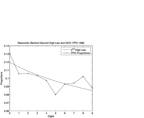
(b) Puerto Rico Elections 1996 PPD Party.

(c) Puerto Rico Elections 1996 PIP Party.

Figure 8: Puerto Rico 1996 Elections compared with the Newcomb–Benford Law for the second digit.

Compliance with the law based on the first digit is to be expected only for greater levels of aggregation, as, for example, in the USA 2004 election on which both the first and second digit laws show impressive fit; see Section 4.1. It should also be emphasized that the results toward NBL are asymptotical in nature, and we require a substantially large numbers of votes to claim a reasonably asymptotic situation, which, only perhaps for the Chicago data, can be claimed among the cases listed by the Carter Center Panel. From an empirical point of view, in this paper we show several elections (with larger data sizes) with good fit to NBL (see Section 4), where compliance with the law is the norm rather than the exception. There is a rapidly increasing number of contributions in which compliance and violations of the NBL have been presented for electoral votes; see Pericchi and Torres (2004), Mebane (2006, 2007a, 2007b), Torres et al. (2007) and Buttorff (2008) among others. (3) A final criticism, raised by the panel appointed by the Carter Center, was that under some (perhaps over simplistic) electoral models, computer simulations did not yield frequencies of second digits in accordance with NBL2. The fact that for some mathematical models NBL2 is not observed may also be regarded as evidence of the lack of realism of such models, and more sophisticated idealizations ought to be searched. In Taylor (2005, 2009) (who was part of the Carter Center Panel) a very intriguing and brief discussion is made of the Newcomb–Benford law regarding elections. The claim is made that the NBL is of “little use in fraud detection” for elections. However, the rationalization covers only the first digit NBL and not the second digit. Data is simulated from models that can be criticized for not being realistic, since realistic population voting models should not be homogeneous on each electoral unit, but should be mixtures of different populations (see next paragraph). The claim seems to be that the results of the simulations contradict NBL for the first, second and third digit laws. However, no measures of fit are provided, and intriguingly, the figures that cover the second and third digits have only 9 entries, although there are 10 second and third digits. (See Taylor, 2005, Figure 8, page 23, Technical Report version November, 7, 2005). Furthermore, for the second digit at least, the fit of the votes for and against the government appear to be markedly different, a fact that is not discussed in the cited Technical Report.

The negative criticism of the Carter Center Panel did not convince everybody. Acknowledging our original suggestion and the Carter Center Report, Walter Mebane presented an invited conference at the Annual Meeting of the American Association for the Advancement of Science which was reported in The Economist (US) (2007), on which the suggestive term “Election Forensics” was coined by Mebane. He provides further support to the use of the 2nd digit NBL (calling it 2BL) for an initial quick scrutiny of elections based solely on officially reported data on the current election and does not require the use of covariates (Mebane, 2006). Mebane produced simulations from realistic models of electorate behavior which are consistent with the 2nd digit NBL, and also presented different types of frauds that are detected by tests on the 2nd digit NBL (although not all frauds are detected). His models are an interesting reflection of political behavior, which are hierarchical mixed population models, denoted here HMPM. In these models there are two populations of voters at each polling station: the partisan population strongly in favor of a candidate and the general population, swinging between candidates. There was, however, a question about the general applicability of the 2nd digit Law: Mebane’s models produce frequencies according to NBL2 for some numbers of voters per unit, say, 2000 or 3000 voters per electoral unit, but not for others, say, 2250. We introduced the Restricted Newcomb–Benford Law (RNBL) in Torres Núñez (2006), before being aware of Mebane’s models. It turns out that the RNBL2 is consistent generally with Mebane’s models, which is illustrated in Table 4.

The NBL1 has been utilized before to check, for example, tax fraud (Nigrini, 1995), and microarrays data corruption (Torres Núñez, 2006). Its use for elections is timely, since electronic voting is raising fresh concerns about the possibility of massive interference with the digital data (Pericchi and Torres, 2004).

The official electoral data, when not presented with levels of aggregation, may have a small upper bound, namely, the number of potential voters. In that respect, when necessary, we proceed in two ways: (1) Check the second digit number Law instead of the first, because the second digit is far less affected, if at all by restrictions on the total; (2) If (1) fails, try the restricted second digit law RNBL with realistic upper bounds; see next section. If both fail, then the alarm is on and further study is required.

The empirical general picture that emerges is that the fit of NBL is accepted in the elections in USA in Puerto Rico and in the manual elections in Venezuela. (In USA 2004, even the first digit and the more complex joint first and second digit test accepts NBL without restrictions). Electronic voting in Venezuela, in the recall referendum, however, fails the test and, to some extent, in the previous presidential elections, adding to the suspicions about electronic voting, particularly without universal paper checking and audits, prior to the sending of the data to the central polling station.

This paper is organized as follows: Section 2 is devoted to the description of the law and a generalization. Section 3 discusses different methods, alternative to the use of $p$-values to judge the fit of the models. Section 4 presents the data analysis of the USA, Puerto Rico and Venezuelan elections and Venezuelan recall referendum. Section 5 states some conclusions.

Table 1: Newcomb–Benford Law for the first significant digit

Digit unit	$\bolds{1}$	$\bolds{2}$	$\bolds{3}$	$\bolds{4}$	$\bolds{5}$	$\bolds{6}$	$\bolds{7}$	$\bolds{8}$	$\bolds{9}$
Probability	0.301	0.176	0.125	0.097	0.079	0.067	0.058	0.051	0.046

Table 2: Newcomb–Benford Law for the second significant digit

Digit unit	$\bolds{0}$	$\bolds{1}$	$\bolds{2}$	$\bolds{3}$	$\bolds{4}$	$\bolds{5}$	$\bolds{6}$	$\bolds{7}$	$\bolds{8}$	$\bolds{9}$
Probability	0.120	0.114	0.109	0.104	0.100	0.097	0.093	0.090	0.088	0.085

2 Overview on the Newcomb–Benford Framework

Intuitively, most people assume that in a string of numbers sampled randomly from some body of data, the first nonzero digit could be any number from 1 through 9, with all nine numbers being equally probable. Empirically, however, it has been found that a law first discovered by Newcomb and later popularized by Benford is ubiquitous.

For the first and second digit Newcomb–Benford Laws we have discrete probability distribution values presented in Table 1 and Table 2, respectively, which are quite different from the Uniform Distribution.

The most general probabilistic justification of the NBL is in Hill (1996).

Hill developed the probability theory that justifies the asymptotic validity of the law for data such as people counts, which do not have units like grams or meters.

The aim here is to use and generalize the Newcomb–Benford Law in order to apply it to wider classes of data sets, particularly arising from elections and to verify their fit to different sets of data with Bayesian statistical methods.

The general definition of the Newcomb–Benford Law is stated here, on base 10, for simplicity. First we introduce the simpler laws for the first and second significant digits. Let $D_{1},D_{2},\ldots$ denote the significant digit functions. For example, $D_{2}(0.154)=5$ gives the second significant digit:

$$p^{B}_{1}(d_{1}) = \mathit{Prob}(D_{1}=\mbox{First significant digit}=d_{1})$$

$$= \log_{10}(1+1/d_{1}),\qquad d_{1}=1,2,\ldots,9,$$

$$p^{B}_{2}(d_{2}) = \mathit{Prob}(D_{2}=\mbox{Second significant digit}=d_{2})$$

$$= \sum_{j=1}^{9}\log_{10}\bigl{(}1+1/(10j+d_{2})\bigr{)},$$

$$\eqntext{d_{2}=0,1,\ldots,9.}$$ (1)

For all positive integers $k$, all $d_{1}\in{\{1,\ldots,9\}}$ and $d_{j}\in{\{0,1,\ldots,9\}}$ for $j=2,\ldots,k$ the joint Newcomb–Benford distribution is

$$p^{B}_{1,\ldots,k}(d_{1},\ldots,d_{k}) = \mathit{Prob}(D_{1}=d_{1},\ldots,D_{k}=d_{k})$$

$$= \log_{10}\biggl{[}1+\frac{1}{\sum_{i=1}^{k}d_{i}\cdot 10^{(k-i)}}\biggr{]}.$$

In the remainder of this section we postulate the way in which the N–B Law acts under restrictions, when the number of electors per electoral unit is restricted to be smaller than a relatively small and known number $K$. This may be important when official data have not been aggregated. The notation used in the following discussion is:

1. $p_{i}^{B}(d_{i})$ is the Newcomb–Benford Probability Distribution for the digit $i$ and number $d_{i}$. These are presented in Table 1 and Table 2 for the first ($i=1$) and second significant digit ($i=2$) respectively.

2. $p_{i}^{C}(d_{i})$ under the constraint $N\leq K$ is the proportion of the numbers with $i$th-digit equals to $d_{i}$ in the set of numbers that are smaller or equal to $K$, that is, $p_{i}^{C}(d_{i})=\frac{\sharp{d_{i}\leq K}}{K}$, where $\sharp{d_{i}\leq K}$ is the cardinality of numbers with $i$th-digit equal to $d_{i}$ that are no bigger than $K$;

3. $p^{U}_{i}(d_{i})$ the proportion of numbers with $i$th-digit equal to $d_{i}$ if no constraints were present.

Note that if there is no restriction, then $p^{C}=p^{U}$. However, if $K=800$, for example, then for the first significant digit, $p_{1}^{B}(d_{1}=2)=0.176$ (see Table 1), $p_{1}^{C}(d_{1}=2)=\frac{111}{800}$ and $p_{1}^{U}(d_{1}=2)=\frac{1}{9}$.

Table 3: NBL for first and second digit with and without an upper restriction of 800

	$\bolds{0}$	$\bolds{1}$	$\bolds{2}$	$\bolds{3}$	$\bolds{4}$	$\bolds{5}$	$\bolds{6}$	$\bolds{7}$	$\bolds{8}$	$\bolds{9}$
$\mathit{NB}1$		0.301	0.176	0.125	0.097	0.079	0.067	0.058	$0.0512$	0.046
$\mathit{CNB}1_{800}$		0.330	0.193	0.137	0.106	0.087	0.073	0.064	$0.006$	0.005
$\mathit{NB}2$	0.120	0.114	0.109	0.104	0.100	0.097	0.093	0.090	$0.088$	0.085
$\mathit{CNB}2_{800}$	0.121	0.114	0.109	0.104	0.100	0.097	0.093	0.090	$0.087$	0.085

Definition 2.1.

The Restricted N–B Law(RNBL) distribution is

$$\qquad p_{i}(d_{i}|N\leq K)=\frac{p_{i}^{B}(d_{i}){p^{C}_{i}(d_{i})}/{p_{i}^{U}(d_{i})}}{\sum_{d_{i}^{\prime}}p_{i}^{B}(d^{\prime}_{i}){p^{C}_{i}(d^{\prime}_{i})}/{p^{U}_{i}(d^{\prime}_{i})}}.$$ (2)

The heuristics behind the RNBL is as follows: sample from sets of numbers that obey NBL, but reject the number if and only if it does not obey the restriction. Note that if $p_{i}^{C}\equiv p_{i}^{U}$, then the usual Newcomb–Benford Law (NBL) is recovered, whether there is a restriction or not. Take as an example the first digit law. If the numbers are restricted to be less than or equal to $K=9$, there is no correction to the NBL. But if $K=15$, say, a substantial correction applies. Note also that the restricted rule is also valid for lower bound restrictions of the form $N\geq K$ or even for two sided restrictions.

For positive numbers, there is a simpler expression for the equation above in terms of the cardinality of the sets induced by the restriction. It turns out that $p^{U}_{i}(d^{\prime}_{i})=\mathit{constant}$ (the constant is equal to $1/9$ for the first digit and to $1/10$ for the second digit). This fact allows to cancel out $p^{U}_{i}$ in (2). Now let $\sharp{d_{i}\leq K}$ be the number of positive numbers less than or equal to $K$, with the $i$th-significant digit equal to $d_{i}$. We may now simplify (2) as follows:

$$p_{i}(d_{i}|N\leq K) = \frac{p_{i}^{B}(d_{i}){p_{i}^{C}(d_{i})}/{p_{i}^{U}(d_{i})}}{\sum_{d_{i}^{\prime}}p_{i}^{B}(d_{i}^{\prime}){p_{i}^{C}(d_{i}^{\prime})}/{p_{i}^{U}(d_{i}^{\prime})}}$$

canceling $$p^{U}_{i}=c$$

$$= \frac{p_{i}^{B}(d_{i})p_{i}^{C}(d_{i})}{\sum_{d_{i}^{\prime}}p^{B}_{i}(d_{i}^{\prime})p_{i}^{C}(d_{i}^{\prime})}$$

$$= \frac{p_{i}^{B}(d_{i}){\sharp\{d_{i}\leq K\}}/{K}}{\sum_{d_{i}^{\prime}}p_{i}^{B}(d^{\prime}_{i}){\sharp\{d_{i}^{\prime}\leq K\}}/{K}}$$

$${}\mbox{canceling }K$$

$$= \frac{p_{i}^{B}(d_{i})\sharp\{d_{i}\leq K\}}{\sum_{d_{i}^{\prime}}p_{i}^{B}(d_{i}^{\prime})\sharp\{d_{i}^{\prime}\leq K\}}.$$

This is a simpler expression easier to calculate.

Comment 1.

In Table 3 we calculated the restricted law with an upper bound of 800. There it is seen that the first digit is more affected by the constraint than the second digit, illustrating that the second digit NBL is of wider applicability than the first digit NBL.

Mebane (2006, 2007a, 2007b) introduced realistic models (HMPM models) of electoral behavior that produced frequencies consistent with the NBL2 for some numbers of electors per unit, like 2000, but not for other such as 2250.

Table 4 displays a large simulation with expected maximum number of voters of 2250 which shows the second digit RNBL to be more consistent with HMPM models than the usual second digit NBL, as anticipated.

Table 4: Table with an upper bound of $N=2250$ voters, that illustrates the better fit of the restricted law, over $m=999$ simulations

	$\bolds{m}$	$\bolds{P(H_{0}|\mathit{data})}$	$\bolds{p}$-values	$\bolds{\underline{P}(H_{0}|\mathit{data})}$
No restrictions	999	0.9996	0.001	000.018
Restrictions	999	1.0000	0.802	$>0.5$

3 Changing $p$-Values to Null Hypothesis Probabilities

The $p$-value is the probability of getting values of the test statistic as extreme as or more extreme than the value actually observed given that the null hypothesis is true. For the first significant digit, the observed chi-squared statistic $\chi^{2}_{\mathit{Observed}}$ is given by

$$\quad\hskip 18.0pt\chi^{2}_{\mathit{Observed}}$$

(3)

$$\qquad\hskip 18.0pt=\mbox{Sample size}\times\sum_{d=1}^{9}\frac{(\mathit{Prob}(D_{1}=d)-f_{d})^{2}}{\mathit{Prob}(D_{1}=d)},$$

where $f_{d}$ is the proportion observed of the digit $d$ as the first significant digit. For the second significant digit, $D_{2}=d\in{\{0,1,\ldots,9\}.}$ This is the basis of a classical test of the null hypothesis which is that the data follows the Newcomb–Benford Law. If the null hypothesis is accepted, the data “passed” the test. If not, a sort of inconsistency has been found which opens the possibility of manipulation of the data. In the electoral process the null hypothesis is $H_{0}{}\dvtx{}$The data is consistent with the Newcomb–Benford proportions for the second significant digit (in Table 2), while the alternative $H_{1}$ means that there is an inconsistency with the law. It is important to get a quantification of the evidence in favor of the Null Hypothesis. In our case, if the data obeys Newcomb–Benford’s Law, then the test offers no basis to suspect undue intervention in the electoral process.

There is a well known statistical misunderstanding between the probability that the null hypothesis is true and the $p$-value. One general way to calibrate $p$-values is through the Universal Upper Bound, due to Sellke, Bayarri and Berger (2001). For a null hypotheses, $H_{0}$, we have

$$P_{val}=\mathit{Prob}(\chi^{2}_{\nu}\geq\chi^{2}_{\mathit{Observed}}|\mbox{ null hypothesis is true}),$$

where $\nu$ is the degrees of freedom, which is equal to 8 for the first significant digit and 9 for the second and onward. If the $p$-value is small (Ex. $p$-values${}<0.05$ or less), it is assumed, based on uncritical practice and convention, that there is a significant result. But the $p$-value is not the probability that the sample arose from the null hypothesis and, therefore, it should not be interpreted as a probability. The usefulness and interpretation of a $p$-value is drastically affected by the sample size.

A useful way to calibrate a $p$-value, under a Robust Bayesian perspective, is by using the bound that is found as the minimum posterior probability of $H_{0}$ that is obtained by changing the priors over large classes of priors under the alternative hypothesis. If a priori we have equal prior probabilities for the two hypotheses, $P(H_{0})=P(H_{1})=1/2$, and for $p_{val}<e^{-1}$, then

$$P(H_{0}|P_{val})$$

(4)

$$\quad\geq 1/\bigl{(}1+[-e\cdot p_{val}\cdot\log_{e}(p_{val})]^{-1}\bigr{)}.$$

A full discussion about this matters can be found in Sellke, Bayarri and Berger (2001).

=6cm $\bolds{p_{\mathit{val}}}$ $\bolds{\underline{P}(H_{0}|\mathit{data})}$ 0.05 $0.29$ 0.01 $0.11$ 0.001 $0.0184$

Table 5: $p$-values in terms of Hypotheses probabilities

It is more appropriate to report the Universal Lower Bound (3) than the $p$-value, with respect to the goodness of fit test of the proportions in the observed digits versus those proportions specified by the Newcomb–Benford Law. As we can see in Table 5, the correction is quite important. This table shows how much larger this lower bound is than the $p$-values. Small $p$-values (i.e., $p_{val}=0.05$) imply that the posterior probability of the null hypotheses is at least $0.29$, which is not very strong evidence to reject a null hypothesis.

However, the lower bound correction does not depend on sample size, so for large sample sizes it can be very conservative. For a full correction of $p$-values, a Bayes Factor is needed, with the corresponding posterior probability of the null hypothesis. Next we compute a very simple Bayes Factor, based on a Uniform prior.

3.1 Posterior Probabilities with Uniform Priors

Let $\Upsilon_{1}=[1,2,\ldots,8,9]$ and $\Upsilon_{2}=[0,1,\ldots,8,9]$.The elements that may appear when the first digit is observed are members of $\Upsilon_{1}$ and if we observe the second digit or higher, the observations are members of $\Upsilon_{2}$. Let

$$\Omega_{0} = \Biggl{\{}p_{1}=p_{01},p_{2}=p_{02},\ldots,$$

$${}\hskip 19.0ptp_{k}=p_{0k}\Big{|}\sum_{i=1}^{k}p_{0i}=1\Biggr{\}}$$

for $k=1,\ldots,9$ in the case of the first digit and $k=0,1,\ldots,9$ for the second digit. Then our hypothesis can be written as

$$\matrix{H_{0}=\Omega_{0},\cr H_{1}=\Omega_{0}^{{}^{\prime}},}$$ (5)

where $\Omega_{0}^{{}^{\prime}}$ means the complement of $\Omega_{0}$. In other words,

$$\Omega_{0}^{{}^{\prime}}=\{p_{i}\neq p_{0i}\mbox{ for at least one }i\in\Upsilon\}.$$

As the simplest objective prior distribution assume an uniform prior for the values of the $p_{i}^{\prime}s$, then

$$\pi^{u}(p_{1},p_{2},\ldots,p_{k}) = \mathit{constant}=\Gamma(k)$$

$$= (k-1)!,$$

which is the correct normalization constant, as it is seen from the well-known integral $\int_{\Omega}\,dp_{1}\cdots dp_{k-1}=1/\Gamma(k)$.

We can write the posterior probability of $H_{0}$ in terms of the Bayes Factor. Let $\mathbf{x}$ be the data vector, then the Bayes Factor is

$$B_{01}=\frac{P(H_{0}|\mathbf{x})P(H_{1})}{P(H_{1}|\mathbf{x})P(H_{0})}.$$ (7)

If we have nested models and $P(H_{0})=P(H_{1})=\frac{1}{2}$, then the Bayes Factor reduces to

$$B_{01}=\frac{P(H_{0}|\mathbf{x})}{P(H_{1}|\mathbf{x})},$$ (8)

where

$$P(H_{0}|\mathbf{x})=\frac{B_{01}}{B_{01}+1}.$$ (9)

For the $i$th significant digit, the data vector is $\textbf{n}=(n_{1},n_{2},\ldots,n_{k})$, where $n_{d}$ is the frequency withwhich $d$ is the $i$th significant digit in the data. Using the definition of a Bayes Factor with a simple hypothesis, we have

$$B_{01} = {f(n_{1},\ldots,n_{k}|\Omega_{0})}$$

$${}\big{/}\biggl{(}\int_{\Omega_{0}^{{}^{\prime}}}f(n_{1},\ldots,n_{k}|\Omega_{0}^{{}^{\prime}})$$

$${}\hskip 30.0pt\cdot\pi^{U}(p_{1},\ldots,p_{k})\,dp_{1}\cdots\,dp_{k-1}\biggr{)},$$

with $\sum_{i\in\Upsilon}p_{i}=1$ and $p_{i}\geq 0\ \forall i\in\Upsilon$. Substituting our assumptions,

$$B_{01}$$

$$\quad=\frac{n!}{\prod_{i=1}^{k}n_{i}!}\prod_{i=1}^{k}p_{i0}^{n_{i}}$$

$$\qquad{}\bigg{/}\Biggl{(}(k-1)!\int_{-\infty}^{+\infty}\frac{n!}{\prod_{i=1}^{k}n_{i}!}$$

$$\qquad\hskip 76.0pt{}\cdot\prod_{i=1}^{k}p_{i}^{n_{i}+1-1}\,dp_{1}\cdots\,dp_{k-1}\Biggr{)}.$$

After canceling factorial terms and using the identity

$$\int_{-\infty}^{+\infty}\prod_{i=1}^{k}p_{i}^{n_{i}+1-1}\,dp_{1}\cdots\,dp_{k}=\frac{\prod_{i=1}^{k}\Gamma(n_{i}+1)}{\Gamma(n+k)},$$

we obtain a simplified expression for $B_{01}$,

$$\hskip 10.0ptB_{01}=\frac{p_{10}^{n_{1}}p_{20}^{n_{2}}\cdots p_{k0}^{n_{k}}}{(k-1)!{\prod_{i=1}^{k}\Gamma(n_{i}+1)}/{\Gamma(n+k)}}.$$ (10)

To obtain the posterior probability using the Bayes Factor (using 9) and substituting $B_{01}$, we get

$$\hskip 22.0ptP(H_{0}|\mathbf{x})$$

$$\hskip 22.0pt\quad={p_{10}^{n_{1}}p_{20}^{n_{2}}\cdots p_{k0}^{n_{k}}}\big{/}\biggl{(}{(k-1)!\frac{\prod_{i=1}^{k}\Gamma(n_{i}+1)}{\Gamma(n+k)}}\biggr{)}$$

(11)

$$\hskip 22.0pt\qquad{}\Big{/}\biggl{(}{p_{10}^{n_{1}}p_{20}^{n_{2}}\cdots p_{k0}^{n_{k}}}$$

$$\qquad\hskip 38.0pt{}\big{/}\biggl{(}(k-1)!\frac{\prod_{i=1}^{k}\Gamma(n_{i}+1)}{\Gamma(n+k)}\biggr{)}+1\biggr{)}.$$

In Torres Núñez (2006), calculations of posterior probabilities with several other priors and approximations are presented. The conclusions are similar to those presented here. [See Berger and Pericchi (2001) for priors and approximations in Bayesian Models Selection].

Table 6: Summary USA 2004 Elections

United States 2004	Min	1st Qu.	Median	Mean	3rd Qu.	Max.
Bush votes	2	$1816$	$5047$	$18380$	$14130$	1076000
Kerry votes	3	$973.2$	$3225.0$	$16840.0$	$9156.0$	1908000
Nader votes	1	$13$	$31$	$143.7$	$85$	13251

Table 7: USA 2004 Elections

United States 2004	$\bolds{m}$	Median	$\bolds{P(H_{0}|\mathit{data})}$	$\bolds{p}$-values	$\bolds{\underline{P}(H_{0}|\mathit{data})}$
NB1 Bush votes	4715	$3694$	1.000	0.003	$0.050$
NB1 Kerry votes	4714	$2603$	1.000	0.002	$0.034$
NB1 Nader votes	2822	$8$	1.000	0.833	$>$ 0.5
NB2 Bush votes	4708	$3713$	1.000	0.068	$0.331$
NB2 Kerry votes	4698	$2621$	1.000	0.651	$>$ 0.5
NB2 Nader votes	2271	$44$	1.000	0.830	$>$ 0.5

4 Results and Data Analysis

We illustrate the use of the First and Second digit Newcomb–Benford Law with data from the 2004 USA elections, three elections in Puerto Rico and the Presidential Recall referendum in Venezuela and one previous Presidential election in that country. We denote by NB1 and NB2 the analysis according to the first and second digit NBL, respectively. We show in the tables the value $m$ which denotes the number of electoral units, and the median number of votes for the respective candidate on the information units. There is wide variation on the aggregation of the numbers, with the USA case as the most aggregate, and Venezuela the least aggregate. That is the reason why the first digit law is obeyed only in the USA, and the fit is remarkable. In most cases, the second digit law is also obeyed, without the need to use the restricted NBL. The case in which the NBL2 was overwhelmingly violated is presented by the Venezuelan Presidential recall vote. We attempted to mend it by restricting the Law for various plausible upper bounds, but the fit did not improve.

4.1 United States Elections 2004

The first case in point is the 2004 USA presidential election, Tables 6 and 7 and Figures 1–7. The data at the level of counties can be found at http:// us.cnn.com/ELECTION/2004/pages/results/.

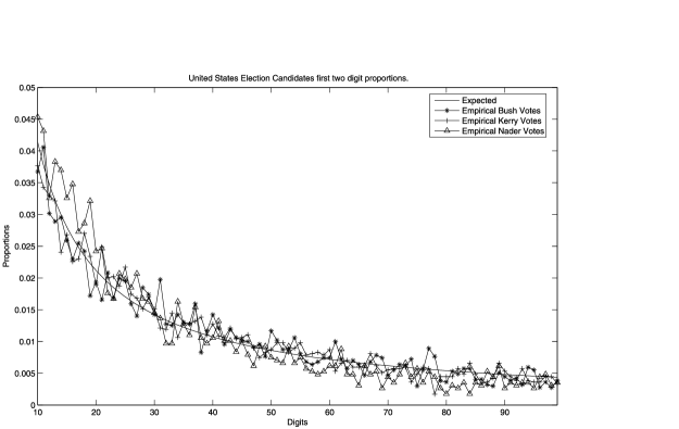
Figure 1: Empirical distributions of the first two digits of the presidential candidates vs. N–B Law for the first two digits.

Figure 2: Bush’s digit proportions vs N–B Law for the $1$st digit.

Figure 3: Kerry’s digit proportions vs. N–B Law for the $1$st digit.

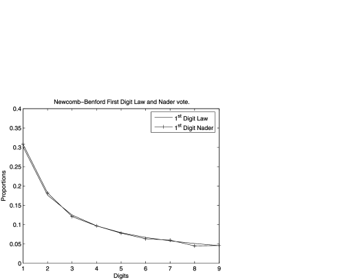
Figure 4: Nader’s digit proportions vs N–B Law for the $1$st digit.

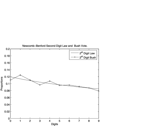
Figure 5: Bush’s digit proportions vs. N–B Law for the $2$nd digit.

Figure 6: Kerry’s digit proportions vs. N–B Law for the $2$nd digit.

Figure 7: Nader’s digit proportions vs. N–B Law for the $2$nd digit.

(Note: Nader’s votes had to be constructed from alternative sources.) This is one of the best case studies we know about the inadequacy of $p$-values when compared to the impressive fit of the NBL with both the first and the second digit, and even with the joint density of first and second digit. For example, in the case of Bush’s votes, for the first digit the fit is excellent, but the $p$-value is only $0.003$, significant even at $0.01$ level. On the other hand, the absolute minimum of posterior probabilities of the null hypothesis is $0.05$, over sixteen times the $p$-value. Note that this is only a lower bound over all possible prior distributions, which is certainly understating the true evidence. Not surprisingly, a real Bayes Factor leads to a posterior probability of almost one.

The best fit is Nader’s votes, which is not significant, neither for the first or the second digit NBL, and so not surprisingly, the posterior probabilities of compliance with NBL is one. Bush’s and Kerry’s votes first digit tests are significant with small $p$-values, but the posterior probabilities are virtually one. For the second digit law the fit in all these cases is excellent. This is illustrated by Figures 1–7.

4.2 Puerto Rico

Here we show the data for the three main parties (PNP, PPD and PIP) in the 1996, 2000 and 2004 elections for governor. The data can be found at http://electionspuertorico.org/datos/2004and http://www.ceepur.org/elecciones2000/.

The results about the first digit are significant. Moreover, the posterior probabilities also reject the NBL1. The restricted NBL for the first digit does not show a big improvement either. This may be due to the fact that in electoral processes, the upper bounds (the total number of electors per polling station) is not typically fixed across the population of polling stations. However, the second digit shows an excellent fit to the NBL2 Law, and the results with restrictions do not change much, illustrating again that the effect of bounds in the second digit is usually smaller than for the first digit NBL.

4.3 Venezuela

4.3.1 Referendum

The 2004 Presidential Revocatory Referendum in Venezuela has attracted considerable interest and controversy. (Data from the Refe-rendum can be found at http://www.cne.gob.ve,http://www.venezuela-referendum.com, https:// sites.google.com/a/upr.edu/probability-and- statistics/data-files-1, http://esdata.info/ 2004.)

One of the most interesting features of this process is that it was partly manual and partly electronic, with the majority of the polling stations having electronic voting, but a sizeable proportion being manual. Here, NO means in favor of the President and SI against.

The most salient feature is that the electronic NO votes give evidence against NB2 Law. Figure 11 shows that the second digits seem to be Uniformly distributed. This is not the case for manual votes, or for the SI electronic votes. This finding is quite informative: The electronic votes in favor of the government need closer scrutiny.

= Puerto Rico 1996 $\bolds{m}$ $\bolds{P(H_{0}|\mathit{data})}$ $\bolds{p}$-values $\bolds{\underline{P}(H_{0}|\mathit{data})}$ NB2 PNP 1836 1.000 0.554 $>0.5$00 NB2 PPD 1839 1.000 0.138 0.0.426 NB2 PIP 1466 1.000 0.104 0.0.390

Table 8: Results of the 1996 Governor Elections in Puerto Rico

= Puerto Rico 2000 $\bolds{m}$ $\bolds{P(H_{0}|\mathit{data})}$ $\bolds{p}$-values $\bolds{\underline{P}(H_{0}|\mathit{data})}$ NB2 PNP 1823 1.000 0.979 $>0.5$ NB2 PPD 1878 1.000 0.436 $>0.5$ NB2 PIP 1579 1.000 0.450 $>0.5$

Table 9: Results of the 2000 Governor Elections in Puerto Rico

= Puerto Rico 2004 $\bolds{m}$ $\bolds{P(H_{0}|\mathit{data})}$ $\bolds{p}$-values $\bolds{\underline{P}(H_{0}|\mathit{data})}$ NB2 PPD 1924 1.000 0.154 $>0.$ 0.44000. NB2 PND 1917 1.000 0.538 $>0.5$00. NB2 PIP 1402 1.000 0.822 $>0.5$00.

Table 10: Results of the 2004 Governor Elections in Puerto Rico

4.3.2 Venezuela 2000

For comparison purposesthe Venezuelan presidential election of 2000 (the presidential election previous to the recall referendum of 2004) is presented here. (Data can be found in: https://sites.google.com/a/upr.edu/probability-and-statistics/data-files-1, http://esdata.info/downloads/ELECCIONES2000.zip.)

(a) Puerto Rico Elections 1996 PNP Party.

(a) Puerto Rico Elections 2000 PNP Party.

(b) Puerto Rico Elections 2000 PPD Party.

(c) Puerto Rico Elections 2000 PIP Party.

Figure 9: Puerto Rico 2000 Elections compared with the Newcomb–Benford Law for the second digit.

(a) Puerto Rico Elections 2004 PNP Party.

(b) Puerto Rico Elections 2004 PPD Party.

(c) Puerto Rico Elections 2004 PIP Party.

Figure 10: Puerto Rico 2004 Elections compared with the Newcomb–Benford Law for the first digit.

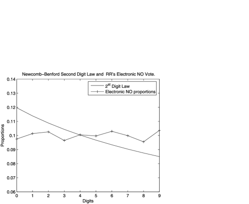
Figure 11: Venezuela Revocatory Referendum Electronic NO Votes proportions. Venezuela Revocatory Referendum Electronic Votes Proportions compared with the Newcomb–Benford Law’s proportions for Second digit. This is the only compelling rejection of the NBL2 law.

Figure 12: Venezuela Revocatory Referendum Electronic SI Votes proportions. Venezuela Revocatory Referendum Electronic Votes Proportions compared with the Newcomb–Benford Law’s proportions for Second digit.

Figure 13: Venezuela Revocatory Referendum Electronic NO Votes proportions. Venezuela Revocatory Referendum Manual Votes Proportions compared with the Newcomb–Benford Law’s proportions for Second digit.

Figure 14: Venezuela Revocatory Referendum Electronic SI Votes proportions. Venezuela Revocatory Referendum Manual Votes Proportions compared with the Newcomb–Benford Law’s proportions for Second digit.

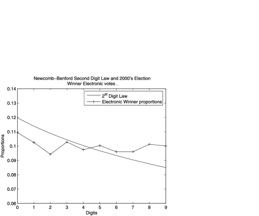
Figure 15: Venezuela 2000 Election Electronic Votes in favor of the Winner compares with Newcomb–Benford Law’s proportions for Second digit.

Figure 16: Venezuela 2000 Election Manual Votes proportions in favor of Winner compares with Newcomb–Benford Law’s proportions for Second digit.

Here none of the candidates for either manual or electronic show compelling evidence against the NB2 Law, although the winning electronic voting results in a posterior probability smaller than the others. Although to a lesser extent than in the 2004 referendum, this result may indicate the need for a closer scrutiny of the winning electronic votes.

5 Conclusions

The main conclusions to be reached here are as follows:

1. At a technical level: (i) the RNBL is a substantial generalization of the NBL that enlarges its domain of applications. However, in the electoral processes presented here, the differences in the results with and without the restriction did not change much. This may be due to the fact that there is no constant upper bound, since the total number of electors is not the same for all polling stations. However, it is the case that the second digit law is far less affected by restrictions than the first digit law. (ii) The second digit NBL2 is a useful test for quick detection of anomalous behavior in electronic or manual elections. (iii) The Universal Lower Bound and even more so, Bayes Factors, are appropriate measures of evidence of the fit to the law, and $p$-values are not, particularly for large data sets like the electoral data.

   Table 11: Results of the 2004 Presidential Recall Referendum in Venezuela for electronic votes

   Venezuela RR	$\bolds{m}$	Median	$\bolds{P(H_{0}|\mathit{data})}$	$\bolds{p}$-values	$\bolds{\underline{P}(H_{0}|\mathit{data})}$
   No Electronic NB2	19064	263	0.000	0.000	0.000
   Si Electronic NB2	19063	172	1.000	0.024	0.196

   Table 12: Results of the 2004 Presidential Recall Referendum in Venezuela for Manual votes

   Venezuela RR	$\bolds{m}$	Median	$\bolds{P(H_{0}|\mathit{data})}$	$\bolds{p}$-values	$\bolds{\underline{P}(H_{0}|\mathit{data})}$
   No Manual NB2	4556	$190$	1.000	0.155	0.440
   Si Manual NB2	4379	$76$	1.000	0.003	0.047

   Table 13: Results of the 2000 Election in Venezuela for electronic votes

   Venezuela 2000	$\bolds{m}$	Median	$\bolds{P(H_{0}|\mathit{data})}$	$\bolds{p}$-values	$\bolds{\underline{P}(H_{0}|\mathit{data})}$
   Winner Electronic NB2	6876	486	0.129	0.000	0.000
   Runner up Electronic NB2	6872	265	1.000	0.017	0.160

   Table 14: Results of the 2000 Election in Venezuela for manual votes

   Venezuela 2000	$\bolds{m}$	Median	$\bolds{P(H_{0}|\mathit{data})}$	$\bolds{p}$-values	$\bolds{\underline{P}(H_{0}|\mathit{data})}$
   Winner Manual NB2	3540	$103$	1.000	0.366	$>0.5$
   Runner up Manual NB2	3219	$52$	1.000	0.006	000.081

   

   Figure 17: Venezuela 2000 Election Electronic Votes proportions of the Loser compares with Newcomb–Benford Law’s proportions for Second digit.

   

   Figure 18: Venezuela 2000 Election Manual Votes proportions of the Loser compares with Newcomb–Benford Law’s proportions for Second digit.

2. Regarding the detection of anomalies: (i) the USA 2004 elections show a remarkable fit to the first digit Newcomb–Benford Law, and also to the second digit NBL. All the manual elections show support for the second digit NBL law. (ii) On the other hand, the electronic results of the votes in favor of the NO in the Recall Referendum violate the NB2 law. This is surprising, since the manual votes in favor and against, as well as the electronic votes in favor of the opposition, fit the law reasonably well. In the previous 2000 Venezuelan presidential elections, there is no compelling evidence against the law, although again the electronic results in favor of the winner show only about $13\%$ of posterior probability in favor of the law.

Our methods, particularly the use of the Second Digit Newcomb–Benford Law, add to the increasing literature on measures of surprise and legitimate suspicion on electoral processes, particularly but not restricted to electronic voting. The NBL2, since our original suggestion in 2004, is becoming a standard tool on what has been termed by Mebane as “Election Forensics.”

References

- Benford (1938) Benford, F. (1938). The law of anomalous numbers. Proc. Amer. Philos. Soc. 78 551–572.
- Berger and Pericchi (2001) Berger, J. O. and Pericchi, L. R. (2001). Objective Bayesian methods for model selection: Introduction and comparison (with discussion). In Model Selection 135–207. IMS, Beachwood, OH. \MR2000753
- Buttorff (2008) Buttorff, G. (2008). Detecting fraud in America’s gilded age. Technical report, Univ. Iowa.
- (4) The Carter Center (2005). Observing the Venezuela Presidential Recall Referendum. http://www.cartercenter. org/documents/2020.pdf Comprehensive Report. Feb. 2005.
- The Economist (US) (2007) The Economist. Feb. 24th–March 2nd, 2007. Pages 93–94. Political Science: Election forensics. http://www.economist. com/science/.
- Hill (1995) Hill, T. (1995). Base-invariance implies Benford’s law. Proc. Amer. Math. Soc. 123 887–895. \MR1233974
- Hill (1996) Hill, T. (1996). A statistical derivation of the Significant-Digit Law. Statist. Sci. 10 354–363. \MR1421567
- Mebane (2006) Mebane, W. R. (2006). Election Forensics: The Second-digit Benford’s Law Test and Recent American Presidential Elections. Election Fraud Conference, Salt Lake Ciy, Utah, September 29–30.
- Mebane (2007a) Mebane, W. R. (2007a). Statistics for Digits. 2007 Summer Meeting of the Political Methodology Society, Pennsylvania State Univ., July 18–21.
- Mebane (2007b) Mebane, W. R. (2007b). Evaluating voting systems to improve and verify accuracy. Presented at the Annual Meeting of the American. Association for the Advancement of Science, San Francisco, Feb. 16, 2007. Available at http:// em.fis.unam.mx/~mochan/elecciones/paperMebane.pdf.
- Newcomb (1881) Newcomb S. (1881). Note on the frequency of use of the Different Digits in Natural Numbers. Amer. J. Math. 4 39–40. \MR1505286
- Nigrini (1995) Nigrini, M. (1995). A taxpayer compliance application of Benford’s Law. J. Amer. Taxation Assoc. 18 72–91.
- Pericchi and Torres (2004) Pericchi, L. R. and Torres, D. (2004). La Ley de Newcomb–Benford y sus aplicaciones al Referendum Revocatorio en Venezuela. Reporte Técnico no-definitivo 2a, Octubre 01, 2004. Presented on Sept. 23, 2004 on the Third Universidad Simon Bolivar Seminar on: Statistical Analyses of the Venezuelan Recall Referendum. Available at https://sites.google.com/a/upr.edu/probability- and-statistics/home/techical-reports.
- Pietronero, Tosatti and Vespignani (2001) Pietronero, L., Tosatti, E. and Vespignani, A. (2001). Explaining the uneven distribution of numbers in nature: The Laws of Benford and Zipf. Physica A 293 297–304.
- Raimi (1976) Raimi, R. (1976). The first digit problem. Amer. Math. Monthly 102 322–327. \MR0410850
- Sellke, Bayarri and Berger (2001) Sellke, T., Bayarri, M. J. and Berger, O. J. (2001). Calibration of -values for testing precise null hypotheses. Amer. Statist. 55 62–71. \MR1818723
- Taylor (2005) Taylor, J. (2005). Too many ties? An empirical analysis of the Venezuelan recall referendum counts. Technical report.
- Taylor (2009) Taylor, J. (2009). Too many ties? An empirical analysis of the Venezuelan recall referendum counts. Statist. Sci. To appear.
- Torres Núñez (2006) Torres Núñez D. A. (2006). Newcomb–Benford’s Law Applications to Electoral Processes, Bioinformatics, and the Stock Index. Supervised by L. R. Pericchi. May 2006. MS thesis.
- Torres et al. (2007) Torres, J., Fernandez, S., Gamero, A. and Sola, A. (2007). How do numbers begin? (the first digit law). Eur. J. Phys. 28 L17–L25.