Simultaneous Ultraviolet and Optical Emission-line Profiles of Quasars: Implications for Black Hole Mass Determination

Abstract

The X-shooter instrument on the VLT was used to obtain spectra of seven moderate-redshift quasars simultaneously covering the spectral range $\sim$3000 Å to 2.5 $\mu$m. At $z\approx 1.5$, most of the prominent broad emission lines in the ultraviolet to optical region are captured in their rest frame. We use this unique dataset, which mitigates complications from source variability, to intercompare the line profiles of C IV $\lambda$1549, C III] $\lambda$1909, Mg II $\lambda$2800, and H$\alpha$ and evaluate their implications for black hole mass estimation. We confirm that Mg II and the Balmer lines share similar kinematics and that they deliver mutually consistent black hole mass estimates with minimal internal scatter ($\mathrel{\hbox{\hbox to0.0pt{\hbox{\lower 4.0pt\hbox{$\sim$}}\hss}\hbox{$<$}}}$0.1 dex) using the latest virial mass estimators. Although no virial mass formalism has yet been calibrated for C III], this line does not appear promising for such an application because of the large spread of its velocity width compared to lines of both higher and lower ionization; part of the discrepancy may be due to the difficulty of deblending C III] from its neighboring lines. The situation for C IV is complex and, because of the limited statistics of our small sample, inconclusive. On the one hand, slightly more than half of our sample (4/7) have C IV line widths that correlate reasonably well with H$\alpha$ line widths, and their respective black hole mass estimates agree to within $\sim$0.15 dex. The rest, on the other hand, exhibit exceptionally broad C IV profiles that overestimate virial masses by factors of 2–5 compared to H$\alpha$. As C IV is widely used to study black hole demographics at high redshifts, we urgently need to revisit our analysis with a larger sample.

1 Motivation

Ever since their discovery in the early 1960s, quasars have attracted attention not only as laboratories for exploring extreme regimes in astrophysics, but also because they serve as useful beacons for probing the interstellar and intergalactic medium. With the growing appreciation that central black holes (BHs) are ubiquitous and inextricably tied to galaxy formation and evolution (Cattaneo et al. 2009, and references therein), quasars have gained even greater prominence in their unique role as markers of vigorous BH growth out to the highest accessible redshifts (Mortlock et al. 2011; Treister et al. 2011).

A key development comes from our ability to estimate BH masses for broad-lined (type 1) active galactic nuclei (AGNs), including quasars, using simple parameters that can be extracted from their rest-frame ultraviolet (UV) and optical spectra. The basic premise is that the BH mass can be approximated by the virial product $M_{\rm BH}=fR_{\rm BLR}\Delta V^{2}/G$, where $R_{\rm BLR}$, the radius of the broad-line region (BLR), can be estimated from the radius-luminosity relation calibrated through reverberating mapping experiments (Kaspi et al. 2000, 2005; Bentz et al. 2009), $\Delta V$ is the velocity dispersion of the line-emitting gas that can be measured from the widths of the broad emission lines, $G$ is the gravitational constant, and $f$ is a geometric factor of order unity that accounts for the poorly constrained geometry and kinematics of the BLR. A variety of approaches have been employed to calibrate the virial method for deriving $M_{\rm BH}$ using single-epoch spectra, using different emission lines for different redshift regimes. H$\beta$ is normally the line of choice for low-redshift objects (Kaspi et al. 2000), as it is the principal line for which most reverberation mapping experiments have been done to date, although under some circumstances H$\alpha$ is preferable to H$\beta$ (Greene & Ho 2005b). At intermediate redshifts, 0.75 $\mathrel{\hbox{\hbox to0.0pt{\hbox{\lower 4.0pt\hbox{$\sim$}}\hss}\hbox{$<$}}}$ $z$ $\mathrel{\hbox{\hbox to0.0pt{\hbox{\lower 4.0pt\hbox{$\sim$}}\hss}\hbox{$<$}}}$ 2, McLure & Jarvis (2002) introduced a formalism based on Mg II $\lambda$2800, while C IV $\lambda$1549 is the only viable option for quasars at $z$ $\mathrel{\hbox{\hbox to0.0pt{\hbox{\lower 4.0pt\hbox{$\sim$}}\hss}\hbox{$>$}}}$ 2 (Vestergaard 2002). With the increasing availability of near-infrared (NIR) spectroscopy, these restrictions can now be circumvented by observing the rest-frame optical lines out to high redshift, thereby minimizing the additional uncertainties incurred through the extra layers of intermediary cross-calibrations. Nevertheless, access to NIR spectroscopy is still far from routine, and all extant, large spectral databases used for statistical analyses of AGNs continue to rely on optical surveys.

A number of studies have investigated the robustness of different broad emission lines commonly used to estimate BH masses. The general consensus is that Mg II serves as a reasonably effective substitute for H$\beta$, the local “standard.” H$\beta$ and Mg II, both low-ionization lines, are thought to arise from gas with common physical conditions and presumably from similar locations with similar kinematics. This expectation appears

to hold to a first approximation (McLure & Dunlop 2004; Salviander et al. 2007; McGill et al. 2008; Shen et al. 2008), and whatever small residual differences there might be appear correctable with empirical prescriptions (Onken & Kollmeier 2008) or more refined spectral analysis (Rafiee & Hall 2011). C IV, on the other hand, turns out to be more problematic. While some contend that C IV can be calibrated to deliver useful mass estimates (Vestergaard 2002; Warner et al. 2003; Vestergaard & Peterson 2006; Kelly & Bechtold 2007; Dietrich et al. 2009; Assef et al. 2011), others sound a more pessimistic note. Baskin & Laor (2005) systematically compared the profiles of C IV and H$\beta$ for low-redshift ($z$ $\mathrel{\hbox{\hbox to0.0pt{\hbox{\lower 4.0pt\hbox{$\sim$}}\hss}\hbox{$<$}}}$ 0.5) quasars for which they could locate published optical and archival space-based UV spectra. The two lines agree poorly. Not only does the width of C IV show large and apparently systematic deviations from H$\beta$, but, as long known (Gaskell 1982; Tytler & Fan 1991), the profile of C IV is often highly blueshifted and asymmetric, casting serious doubt as to whether the line properly traces gravitationally bound gas. Netzer et al. (2007), Sulentic et al. (2007), and Shen & Liu (2012) arrive at a similar conclusion from analysis of moderate-redshift ($z\approx 2$) quasars for which they secured rest-frame Balmer line measurements using near-IR spectroscopy; the widths of the Balmer lines exhibit little, if any, correlation with the widths of C IV.

AGNs vary. Larger variations usually occur at shorter wavelengths and in lines of higher ionization. An important limitation of most of the previous studies comes from the fact that the rest-frame UV and optical lines were observed non-simultaneously, often separated widely apart in time (timescales of months to years), making any comparison between them inherently uncertain. The width of C IV in quasars, for instance, changes up to $\sim$30% on timescales of weeks to months (Wilhite et al. 2006a). Fortunately, variability has only a relatively minor impact on BH masses derived from single-epoch spectra. According to Wilhite et al. (2006b), Denney et al. (2009), and Park et al. (2012) variability affects the mass estimates only at the level of $\sim$0.1 dex, which is small, but significant, compared to the $0.3-0.4$ dex error budget that still plagues the various mass estimators (Vestergaard & Peterson 2006; McGill et al. 2008). Still, to achieve a better understanding of how the different lines most commonly used for BH mass estimation compare to each other, it would be highly desirable to perform a comparative analysis using a set of simultaneous rest-frame UV–optical spectra of quasars. This is the main goal of this paper.

Distribution of the continuum luminosity at 3000 Å and the FWHM of the broad component of Mg II $\lambda$2800 for 11,015 SDSS DR7 quasars with $z=1.4-1.6$ (Shen et al. 2011). The objects observed with X-shooter are plotted as red points. The values of FWHM from SDSS were reduced by 0.05 dex to account for the systematic difference in the method used to fit Mg II (Shen et al. 2011).

Figure 1: X-shooter spectra of our sample, shifted to the rest-frame of the objects. We only show the spectral regions that contain the strongest emission lines used for the profile analysis. The individual objects have been shifted by arbitrary constant additive offsets to improve the clarify of the plot.

Distance-dependent quantities are calculated assuming the following cosmological parameters: $H_{0}=100~{}h=71$ km s^-1 Mpc^-1, $\Omega_{m}=0.26$, and $\Omega_{\Lambda}=0.74$ (Komatsu et al.  2009).

2 Observations and Data Reduction

We selected seven relatively bright ($r\approx 18-19$ mag) quasars from the Seventh Data Release of the Sloan Digital Sky Survey (SDSS DR7; Abazajian et al. 2009). As we are interested in simultaneous coverage of C IV $\lambda$1549 to H$\alpha$, we chose the targets to have $z\approx 1.5$. During the selection process, we inspected the existing SDSS spectra to ensure that the objects have unambiguous broad emission lines suitable for estimating BH masses. We avoided sources with obvious broad absorption features, but aside from this, we did not apply any other selection criteria. Figure 1 compares our sample with the distribution of Mg II line widths (FWHM) and 3000 Å continuum luminosity for 11,015 $z=1.4-1.6$ quasars contained in the DR7 catalog of Shen et al. (2011). Our objects are on average slightly less luminous than the peak of the DR7 distribution, but there are no obvious biases. The one apparent outlier with relatively narrow lines is SDSS J122925.95$-$030702.4, which was intentionally included for comparison because it has characteristics similar to narrow-line Seyfert 1 (NLS1) galaxies. Thus, even though our sample is small and somewhat ill-defined, it nonetheless represents an unbiased subset of luminous ($L_{3000}>10^{45.4}$ erg s^-1), moderate-redshift, optically selected quasars.

The observations were made using X-shooter (Vernet et al. 2011), a three-arm, single-object echelle spectrograph that started operations in 2009 October on the VLT. The instrument covers simultaneously the wavelength range from $\sim$3000 Å to 2.40 $\mu$m, in three arms: UVB ($\Delta\lambda=3000-5500$ Å), VIS ($\Delta\lambda=5500$ Å – 1.02 $\mu$m), and NIR ($\Delta\lambda=$ 1.02–2.40 $\mu$m). The data were taken within the framework of the French Guaranteed Time under program 086.B-0320(A) (PI G. Ponti) and took place on 2010 February 18 UT. A summary of the observations is given in Table 1.

For our observations we used slit widths of 1$\farcs$3, 1$\farcs$2, and 1$\farcs$2, respectively, for the three arms, resulting in resolving powers of $R\equiv\lambda/\Delta\lambda\approx$ 4000, 6700, and 4300. The slits were aligned along the parallactic angle. The observations consist of four separate exposures of 450 s each, for a total of 1800 s, for all sources except SDSS J122925.95$-$030702.4, which was observed for 900 s per exposure for a total of 3600 s. The exposures were taken while nodding the object along the slit with an offset of 5^′′ between exposures in a standard ABBA sequence. Every observation was preceded by an observation of an A0 V telluric standard star at similar airmass. The night was not photometric due to the presence of thin clouds. A high, variable humidity was present with precipitable water vapor varying between 5 and 7.5 mm, rather high for Paranal but not exceptional for this period of the year in Chile (so-called “Bolivian winter”).

We processed the spectra using version 1.1.0 of the X-shooter data reduction pipeline (Goldoni et al. 2006), which performed the following actions. As usual in processing nodding observations, the raw frames taken at different positions were differenced with each other to obtain two frames (i.e. A$-$B and B$-$A), on which cosmic ray hits were detected and corrected using the method developed by van Dokkum (2001). The frames were then divided by a master flat field obtained using day-time flat

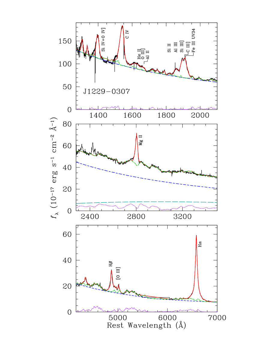
Figure 2: Spectral fitting for one of the objects in our sample, SDSS J1229$-$0307. The original data, corrected for Galactic reddening, are plotted in black histograms. The fitted components include a featureless power law (dashed blue), the Balmer continuum (long dashed turquoise), and iron emission (dotted purple), which altogether constitute the pseudocontinuum (dot-dashed green). The final model, including fits to the principal emission lines, is shown in solid red.

field exposures with halogen lamps. The orders were extracted and rectified in wavelength space using a wavelength solution previously obtained from calibration frames. The resulting rectified orders were then shifted and added to superpose them, thus obtaining the final two-dimensional spectrum. The orders were then merged, and, in the overlapping regions, the merging was weighted by the errors that were propagated during the process. From the resulting two-dimensional, merged spectrum a one-dimensional spectrum was extracted at the source’s position. The one-dimensional spectrum with the corresponding error file and bad pixel map is the final product of the reduction.

To perform flux calibration, we used different procedures for the UVB data and for the VIS-NIR data. In the UVB band we used an observation of the flux standard GD 71 (Bohlin 2007) taken in the beginning of the night. We reduced the data using the same steps as above, but in this case we subtracted the sky emission lines using the method of Kelson (2003). The extracted spectrum was divided by the flux table of the star from the CALSPEC HST database to produce the response function, which was then applied to the spectrum of the science targets. For the VIS and NIR arms, we used A0V stars as both flux and telluric standards. We extracted the A0V spectra with the same procedure used for the flux standard and used these spectra to apply telluric corrections and flux calibrations simultaneously, using the package Spextool (Vacca et al. 2003). We verified that the final spectra of the three arms were compatible in the common wavelength regions and then adjusted the mean continuum flux in the overlap range between 4000 Å and 9000 Å to be consistent with the SDSS spectra, which have a more reliable absolute flux calibration. Figure 2 shows the calibrated, rest-frame spectra of the quasars observed in our program.

3 Spectral Fitting

We correct the X-shooter and SDSS spectra for Galactic extinction using the extinction map of Schlegel et al. (1998) and the reddening curve of Fitzpatrick (1999). The spectra are transformed into the rest frame using the redshift as determined from the peak of the best-fit model (see below) for the [O III] $\lambda 5007$ line. To improve on the absolute flux calibration, we rescale the X-shooter spectra to the flux density level of the SDSS spectra over the wavelength region where the two overlap. Here we present a brief description of the spectral fitting, which is based on $\chi^{2}$-minimization using the Levenberg–Marquardt technique within the MPFIT package (Markwardt 2009).

The analysis for the optical spectra closely follows the methodology for decomposition of AGN spectra described in Dong et al. (2008). We do not correct for starlight contamination, which is expected to be negligible for quasars in our luminosity range ($L_{3000}>10^{45.4}$ erg s^-1). As the broad emission lines, particularly the Fe II multiplets, are so broad and strong that they merge together and essentially leave no line-free wavelength regions, we fit simultaneously the nuclear

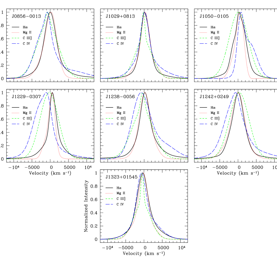
Figure 3: Model line profiles, shown on a velocity scale, for H$\alpha$ $\lambda$6563 (black, solid), Mg II $\lambda$2800 (red, dotted), C III] $\lambda$1909 (green, dashed), and C IV $\lambda$1549 (blue, long dashed). The zero point of the velocity scale is referenced with respect to [O III] $\lambda$5007.

continuum, the Fe II multiplets, and other emission lines. The featureless continuum of type 1 AGNs is not well described by a single power law when a large range of wavelengths is considered (e.g., Vanden Berk et al. 2001). We approximate it by a broken power law, with free indices for the H$\alpha$ and H$\beta$ regions. The optical Fe II emission is modeled with two separate sets of analytical spectral templates, one for the broad-line system and the other for the narrow-line system, constructed from measurements of I Zw 1 by Véron-Cetty et al. (2004). Within each system, the respective set of Fe II lines is assumed to have no relative velocity shifts and the same relative strengths as those in I Zw 1. Emission lines are modeled as multiple Gaussians. Following Dong et al. (2011), we assume that the broad Fe II lines have the same profile as broad H$\alpha$. In our data set, the H$\beta$ region is significantly noisier than the H$\alpha$ region. In our subsequent analysis we will use H$\alpha$ in lieu of H$\beta$; Greene & Ho (2005b) have shown that the broad component of H$\alpha$ is on average slightly narrower than H$\beta$, but the two closely track each other. All narrow emission lines are fitted with a single Gaussian, except for the [O III] $\lambda\lambda 4959,5007$ doublet, each of which is modeled with two Gaussians, one accounting for the line core and the other for a possible blue wing seen in many objects (Greene & Ho 2005a).

For the near-UV spectra, we focus our analysis on the region around Mg II $\lambda\lambda$2796, 2803, following the method described in Wang et al. (2009). Here the pseudocontinuum consists not only of a local power-law continuum and an Fe II template, but also an additional component for the Balmer continuum. The Fe II emission is modeled with the semi-empirical template for I Zw 1 generated by Tsuzuki et al. (2006). To match the width and possible velocity shift of the Fe II lines, we convolve the template with a Gaussian and shift it in velocity space. As in Dietrich et al. (2002), the Balmer continuum is assumed to be produced in partially optically thick clouds with a uniform

Figure 4: Comparison of FWHM of H$\alpha$ with FWHM of (a) Mg II, (b) C IV, and (c) C III]. The error bars represent measurement uncertainties as given in Table 2 (see Section 3).

temperature. Each of the lines of the Mg II doublet is modeled with two components, one broad and the other narrow. The broad component is fit with a truncated, five-parameter Gauss-Hermite series; a single Gaussian is used for the narrow component. The two doublet lines are assumed to have identical profiles, a fixed separation set to the laboratory value, and a flux ratio $\lambda$2796/$\lambda$2803 set to be between 2:1 and 1:1 (Laor et al. 1997).

The fitting for the UV region is performed with a modified version of a code initially written and kindly provided by Jian-Guo Wang. We employ the UV Fe II $+$ Fe III template for I Zw 1 generated by Vestergaard & Wilkes (2001). In light of the moderate signal-to-noise ratio of our data, we adopt the same scaling factor for the Fe II and Fe III emission; this assumption seems adequate from visual inspection of the fits. As in Vestergaard & Wilkes (2001), the power-law continuum and iron emission (both constituting the pseudocontinuum) are fit to the emission-line–free spectral regions from 1300 Å to 2200 Å. After the pseudocontinuum is subtracted, we concentrate our fits on two regions: (1) $\sim 1350-1700$ Å, which contains the blend of Si IV and O IV] at $\sim$1400 Å, C IV $\lambda 1549$, He II $\lambda 1640$, O III] $\lambda 1663$, and Al II $\lambda 1670$, and (2) $\sim 1800-2000$ Å, which covers Si II $\lambda 1817$, Al III $\lambda\lambda 1855,\,1863$, Si III] $\lambda 1892$, C III] $\lambda 1909$, and the Fe III UV34 triplet at $\sim$1914 Å. We model the emission lines with multiple Gaussian components, using the minimum number necessary to achieve a satisfactory fit within the signal-to-noise constraints of the data. The C IV profile is fit with three Gaussians, taking care to avoid narrow absorption features when present (as in J1238$-$0056 and J1323$+$0154; see Figure 2). For the C III] region, Si II, Al III, Si III], and Fe III are each fit with a single Gaussian, while C III] itself is fit with two Gaussians, which in most cases yield better residuals than a single Gaussian. This suffices for our purposes. Our primary objective is to obtain a robust characterization of the profile of C IV and C III], not to achieve a detailed model for every line in this tremendously complicated spectral region.

Figure 3 illustrates the fits for one of objects, and the results of the fits for the entire sample are summarized in Table 2. The emission-line luminosities, velocity shifts (peak of the line; $v$), and velocity widths (FWHMs) are measured from the best-fit models of the line profiles, except for the case of Mg II, whose line peak and FWHM are measured from the model of the single doublet line, Mg II $\lambda$2796. The strength of the optical Fe II $\lambda 4570$ emission is integrated over the wavelength range 4434–4684 Å, and that for UV Fe II is integrated over the range 2200–3090 Å. For all measured emission-line fluxes, we regard the values as reliable detections when they have greater than $3\,\sigma$ significance. As the instrumental resolution (FWHM $\approx 45-75$ km s^-1) is small compared to the measured line widths (FWHM $\approx 500-6000$ km s^-1), no correction for instrumental resolution has been applied to the line widths.

We follow the bootstrap method of Dong et al. (2008; their Section 2.5) to estimate measurement uncertainties. The typical 1 $\sigma$ errors on the fluxes of the strong lines considered in this paper are quite small, $\mathrel{\hbox{\hbox to0.0pt{\hbox{\lower 4.0pt\hbox{$\sim$}}\hss}\hbox{$<$}}}$10% (see Dong et al. 2008, 2011; Wang et al. 2009). We adopt 10% errors for the fluxes of Mg II, C III], and [O III] and 5% for H$\alpha$. The only exception is C IV, whose final flux depends on the exact procedure adopted to fit the “red shelf” (region $\sim 1600-1700$ Å; see, e.g., Fine et al. 2010). We assume that the red shelf is intrinsic to C IV; excluding it reduces the inferred line flux by $\sim$10–25%. To be conservative, we adopt an error of 18% for the flux of C IV. The FWHM values are best measured for H$\alpha$ (error 5%), followed by Mg II (error 10%), C IV (error 15%), and C III] (error 15%–25%). C III] is particularly problematic because of severe blending with Al III $\lambda\lambda 1855,\,1863$, Si III] $\lambda 1892$, and Fe III UV34.

4 Results

Figure 4 shows the final, fitted profiles for the sample, normalized by their amplitude and plotted on a velocity scale. A direct comparison among the line widths is given in Figure 5. Several trends are immediately obvious.

1. H$\alpha$ shows, by far, the most symmetric profiles and the least amount of systemic velocity shift. This is not unexpected, given the overall similarity between H$\alpha$ and H$\beta$ profiles (Greene & Ho 2005b), reinforcing the commonly adopted view that the Balmer lines offer the most reliable BH virial mass estimators (but see Vestergaard et al. 2011 for a different point of view).

2. Consistent with other studies (e.g., McLure & Dunlop 2004; Shen et al. 2008; Shen & Liu 2012), we find that Mg II on average serves as a reasonably decent proxy for the Balmer lines, at least for five out of the seven objects in our sample. The two exceptions are J1050$-$0105 and

   

   Figure 5: Comparison of $M_{\rm BH}$ derived using (a) Mg II and H$\alpha$, (b) C IV and H$\alpha$, and (c) C IV and Mg II. The error bars reflect the statistical uncertainties for the BH mass estimators (see Section 4).

   J1229$-$0307, whose Mg II lines are distinctly narrower than H$\alpha$ and somewhat asymmetric.

3. Among the five objects that show better match between Mg II and H$\alpha$, the lines agree best near the core (FWHM) but often diverge noticeably in the wings. H$\alpha$ generally has more extended wings than Mg II. This implies that comparison between virial mass estimators for Mg II and the Balmer lines depends sensitively on the adopted measure of line width. The agreement should be reasonably close for the FWHM (Figure 5(a); mean and standard deviation $\langle$FWHM(Mg II)/FWHM(H$\alpha$)$\rangle=0.95\pm 0.14$ km s^-1), but the line dispersion, more sensitive to the line wings, will be systematically higher for the Balmer lines compared to Mg II.

4. The behavior of C IV is much more perplexing. Apart from the presence of a prominent extended red wing—a model-dependent feature sensitive to the adopted fitting procedure (Fine et al. 2010)—the line peak exhibits a range of velocity shifts, from $\sim$800 km s^-1 to $-1100$ km s^-1. A direct comparison between C IV and H$\alpha$ line widths reveals two clusters of points (Figure 5(b)). Four of the quasars have C IV line widths that are roughly consistent with those of H$\alpha$ (mean and standard deviation $\langle$FWHM(C IV)/FWHM(H$\alpha$)$\rangle=1.07\pm 0.11$ km s^-1), whereas the other three (J1229$-$0307, J1238$-$0056, and J1242$+$0249) are significantly broader, $\langle$FWHM(C IV)/FWHM(H$\alpha$)$\rangle=1.86\pm 0.38$ km s^-1. Both are difficult to understand in the context of a radially stratified BLR with a velocity field dominated by Keplerian rotation, wherein $\Delta V\propto R_{\rm BLR}^{1/2}$. Not many AGNs have been reverberation mapped in C IV, but the handful for which adequate data exist show that C IV arises from a region that is a factor of $\sim 2$ more compact than H$\beta$ (e.g., Korista et al. 1995; Onken & Peterson 2002). If these results apply to higher luminosity quasars, they imply that FWHM(C IV) $\approx$ $\sqrt{2}$FWHM(H$\alpha$) [for simplicity, we assume FWHM(H$\alpha$) = FWHM(H$\beta$)]. Our sample, albeit small, does not seem to conform to this simple expectation. The three outliers with unusually high FWHM(C IV)/FWHM(H$\alpha$) share one common characteristic: the peak of the C IV is significantly blueshifted, by $-$700 to $-$1100 km s^-1. However, not all objects with C IV blueshifts show enhanced FWHM(C IV)/FWHM(H$\alpha$); two of the other four objects also show blueshifts of comparable magnitude. Nor is excess C IV width uniquely associated with any obvious AGN property. While J1229$-$0307, with its relatively narrow lines [FWHM(H$\alpha$) $\approx$ 2500 km s^-1], strong Fe II emission (log Fe II $\lambda$4570/H$\beta$ = $-0.12$), and high Eddington ratio (log $L_{{\rm bol}}$/$L_{{\rm Edd}}$ = 0.21) qualify it as a NLS1, whose C IV line may be particularly problematic for mass determination (Vestergaard et al. 2011), the other two outliers do not.

5. C III] poses an even greater challenge to understand. While there are no large velocity shifts, the width of C III] appears to be completely erratic (Figure 5(c)). Two of the objects have unusually narrow cores that result in FWHM(C III])/FWHM(H$\alpha$) $<$ 1, and the rest are characterized by FWHM(C III])/FWHM(H$\alpha$) $\gg$ 1. Counterintuitively, FWHM(C III]) $>$ FWHM(C IV) in four out of the seven sources. This agrees with the results of Brotherton et al. (1994), Jiang et al. (2007), and Greene et al. (2010), but is inconsistent with the study of Shang et al. (2007), who generally find FWHM(C III]) $\mathrel{\hbox{\hbox to0.0pt{\hbox{\lower 4.0pt\hbox{$\sim$}}\hss}\hbox{$<$}}}$  FWHM(C IV). Using a much larger sample, Shen & Liu (2012) find no obvious offset between FWHM(C III]) and FWHM(C IV), although the two are poorly correlated. The discrepancy associated with C III] may arise, at least in part, from the uncertainty in deblending the line from its surrounding contaminating features.

How do these results impact BH mass determinations? Figure 6 graphically illustrates the answer. We estimate BH masses using the C IV-based formalism of Vestergaard & Peterson (2006), the Mg II-based formalism of Vestergaard & Osmer (2009), and the H$\alpha$-based formalism of Greene & Ho (2005b), as updated by Xiao et al. (2011) to account for the latest BLR size-luminosity relation of Bentz et al. (2009). For consistency with our adopted C IV and Mg II mass estimators, we further adjust Xiao et al.’s prescription so that its virial coefficient $f$ matches the value advocated by Onken et al. (2004). We do not consider C III] because there is currently no mass estimator based on this line, and we feel discouraged by the line width comparison presented above. The BH masses derived from these virial mass estimators typical have statistical uncertainties of $\sim 0.3-0.4$ dex. For concreteness, we adopt an error bar of 0.4 dex for $M_{\rm BH}$(C IV) and 0.3 dex for both $M_{\rm BH}$(Mg II) and $M_{\rm BH}$(H$\alpha$).

Vestergaard et al. (2011) stress the importance of using mass estimators calibrated on the same mass scale for a proper comparison between masses derived from different lines. Both the C IV and Mg II masses are tied to a common scale based on reverberation-mapped AGNs. Vestergaard & Osmer, however, model the broad Mg II line as a single component, whereas we follow Wang et al. (2009) and treat Mg II as a doublet, which results in slightly narrower line widths. These two methods yield Mg II line widths that differ on average only by $\sim 0.05$ dex (Shen et al. 2011); we scale up all of our Mg II line widths by this constant factor to account for the minor systematic offset. To date the H$\alpha$ BH mass estimator of Greene & Ho (2005b) has not been calibrated directly against the reverberation-mapped AGNs. Fortunately, the analysis of Shen et al. (2011) indicates that the H$\alpha$-based masses show only a mean offset of 0.08 dex with respect to Vestergaard & Peterson’s H$\beta$-based masses, which, like the C IV and Mg II masses, are calibrated to the same scale tied to the reverberation-mapped AGNs. For the purposes of this paper, we will not worry about this small discrepancy, which does not impact any of our main conclusions.

As foreshadowed by the line width analysis, H$\alpha$ and Mg II deliver reasonably consistent mass estimates, which for our sample spans a small range around $M_{\rm BH}\approx 10^{8.7\pm 0.2}$ $M_{\odot}$. For our choice of mass estimators, $M_{\rm BH}$(Mg II) agrees very well with $M_{\rm BH}$(H$\alpha$): $\langle$log $M_{\rm BH}$(Mg II)$-$log $M_{\rm BH}$(H$\alpha$)$\rangle\approx 0.03\pm 0.07$ dex. By contrast, the comparison between $M_{\rm BH}$(C IV) and $M_{\rm BH}$(H$\alpha$) is less clear-cut. The three objects (labeled in Figure 6) with anomalously broad, blueshifted C IV profiles all have $M_{\rm BH}$(C IV) in excess of $10^{9}$ $M_{\odot}$, deviating from $M_{\rm BH}$(H$\alpha$) by 0.34 dex to as much as 0.72 dex. The most discrepant object is the NLS1 J1229$-$0307, confirming Vestergaard et al.’s (2011) suspicion that C IV masses are especially unreliable for this class of AGNs, but the other two show no obvious warning signs as to why C IV should misbehave. All three C IV outliers appear relatively normal in the Mg II versus H$\alpha$ comparison (Figure 6(a)). The remaining four objects fare better: $\langle$log $M_{\rm BH}$(C IV)$-$log $M_{\rm BH}$(H$\alpha$)$\rangle\approx 0.01\pm 0.14$ dex. While this may be regarded as reassuring confirmation that C IV-based masses can be trusted in at least some objects, the difficulty is that, in the absence of independent evidence from lower ionization lines (Mg II, H$\beta$, or H$\alpha$), we have no means of forecasting which objects are reliable or not. This result is unsettling, especially in light of the very large masses ($M_{\rm BH}\approx 10^{9}-10^{10}$ $M_{\odot}$) routinely inferred for high-redshift quasars and the astrophysical implications attached to them.

5 Summary

The widths of broad emission lines in active galaxies, when combined with physical dimensions inferred from the size-luminosity relation empirically calibrated from reverberation mapping experiments, provide a powerful and efficient means of estimating BH masses for large samples of sources detected at all redshifts. Over the past decade, a number of virial BH mass estimators have been devised and extensively used to determine BH masses, facilitating a wide range of investigations on BH demographics and AGN physics. Despite their popularity, however, there are nagging doubts as to the reliability of these mass estimators. While calibrations based on low-ionization lines, especially H$\alpha$ and H$\beta$, are reasonably secure, higher redshift observations often depend on UV lines that are less well understood. The most contentious mass estimator is that based on C IV $\lambda$1549, the workhorse for studies of high-redshift quasars, as the kinematics of this line may be significantly affected by winds and other non-virial motions. Mg II appears to be safer, but even it may not be completely immune to systematic biases.

Spectral variability complicates the comparison between different mass estimators, if they derive from spectra taken at different times. To mitigate this effect, we have undertaken an experiment to acquire spectra of a small sample of seven moderate-redshift quasars that simultaneously cover the rest-frame UV through optical spectral regions (1300–7500 Å). This dataset is enabled by the unique capabilities of the X-shooter instrument on the VLT, which delivers simultaneous spectra from $\sim$3000 Å to 2.5 $\mu$m. At $z\approx 1.5$, this allows us to access the principal broad emission lines from C IV to H$\alpha$.

In accord with other studies, we find that Mg II and the Balmer lines (this study uses H$\alpha$ instead of H$\beta$) have similar velocity widths near the core (FWHM) of their profiles, but H$\alpha$ generally has more extended, higher velocity wings than Mg II. Mg II-based and H$\alpha$-based BH masses agree to better than $\sim 0.1$ dex. The C III] $\lambda$1909 line widths are difficult to interpret. Contrary to naive expectations, FWHM(C III]) $>$ FWHM(C IV) in most of our objects, but some also have unusually narrow lines, narrower than even those of H$\alpha$. While these discrepancies can perhaps be attributed to the difficulties of line deblending in the highly crowded spectral region near $\sim$1900 Å, it appears that it would be challenging to devise a robust BH virial mass estimator using C III]. The verdict on C IV is mixed. While roughly half of the C IV-based masses are reasonably consistent with those derived from H$\alpha$, the others are systematically high by factors of 2–5. These extreme outliers not only have unusually broad C IV line widths, but their line peaks are all systematically blueshifted by several hundred to a thousand km s^-1, suggesting that a significant fraction of the emission arises from outflowing or dynamically unrelaxed gas. However, systemic C IV blueshifts are a common feature in AGNs, and they do not appear to be a clean predictor of which objects show deviant C IV line widths or masses; two of the objects whose C IV-based masses agree with those derived from H$\alpha$ also have systematic C IV blueshifts of comparable magnitude. We are thus left in an uncomfortable predicament: in the absence of independent confirmation from lower ionization lines, we do not know, a priori, which C IV profiles provide more accurate mass estimates.

To end on a more positive note, we emphasize that our results clearly suffer from small-number statistics. Other investigators (e.g., Vestergaard & Peterson 2006; Greene et al. 2010; Assef et al. 2011) are more optimistic that C IV can be used to study BH demographics at high redshifts. It would be important to secure simultaneous, or at least near-contemporaneous, rest-frame UV-optical spectra for a larger, better defined sample of AGNs to revisit the issues raised in this study. Because high-luminosity AGNs vary on time scales of weeks to months, complete simultaneity in spectral coverage (such as those presented here) is desirable, but not truly necessary. Near-contemporaneous observations, taken within a span of a few days (e.g., during the same observing run or coordinated between two different telescopes), would suffice.

References

- (1) Abazajian, K. N., Adelman-McCarthy, J. K., Agüeros, M. A., et al. 2009, ApJS, 182, 543
- (2) Assef, R. J., Denney, K. D., Kochanek, C. S., et al. 2011, ApJ, 742, 93
- (3) Baskin, A., & Laor, A. 2005, MNRAS, 356, 1029
- (4) Bentz, M. C., Peterson, B. M., Netzer, H., Pogge, R. W., & Vestergaard, M. 2009, ApJ, 697, 160
- (5) Bohlin, R. C. 2007, in The Future of Photometric, Spectrophotometric and Polarimetric Standardization, ed. C. Sterken (San Francisco: ASP), 315
- (6) Brotherton, M. S., Wills, B. J., Steidel, C. C., & Sargent, W. L. W. 1994, ApJ, 423, 13
- (7) Cattaneo, A., Faber, S. M., Binney, J., et al. 2009, Nature, 460, 213
- (8) Denney, K. D., Peterson, B. M., Dietrich, M., Vestergaard, M., & Bentz, M. C. 2009, ApJ, 692, 246
- (9) Dietrich, M., Appenzeller, I., Vestergaard, M., & Wagner, S. J. 2002, ApJ, 564, 581
- (10) Dietrich, M., Mathur, S., Grupe, D., & Komossa, S. 2009, ApJ, 696, 1998
- (11) Dong, X.-B., Wang, J.-G., Ho, L. C., et al. 2011, ApJ, 736, 86
- (12) Dong, X., Wang, T., Wang, J., et al. 2008, MNRAS, 383, 581
- (13) Fine, S., Croom, S. M., Bland-Hawthorn, J., et al. 2010, MNRAS, 409, 591
- (14) Fitzpatrick, E. L. 1999, PASP, 111, 63
- (15) Gaskell, C. M. 1982, ApJ, 263
- (16) Goldoni, P., Royer, F., François, P., et al. 2006, SPIE, 6269, 62692
- (17) Greene, J. E., & Ho, L. C. 2005a, ApJ, 627, 721
- (18) Greene, J. E., & Ho, L. C. 2005b, ApJ, 630, 122
- (19) Greene, J. E., Peng, C. Y., & Ludwig, R. R. 2010, ApJ, 709, 937
- (20) Jiang, L., Fan, X., Vestergaard, M., et al. 2007, AJ, 134, 1150
- (21) Kaspi, S., Maoz, D., Netzer, H., et al. 2005, ApJ, 629, 61
- (22) Kaspi, S., Smith, P. S., Netzer, H., et al. 2000, ApJ, 533, 631
- (23) Kelly, B. C., & Bechtold, J. 2007, ApJS, 168, 1
- (24) Kelson, D. D. 2003, PASP, 115, 688
- (25) Komatsu, E., Dunkley, J., Nolta, M. R., et al. 2009, ApJS, 180, 330
- (26) Korista, K. T., Alloin, D., Barr, P., et al. 1995, ApJS, 97, 285
- (27) Laor, A., Jannuzi, B. T., Green, R. F., & Boroson, T. A. 1997, ApJ, 489, 656
- (28) Markwardt, C. B. 2009, in Astronomical Data Analysis Software and Systems XVIII, ed. D. A. Bohlender, D. Durand, & P. Dowler (San Francisco: ASP), 251
- (29) McGill, K. L., Woo, J.-H., Treu, T., & Malkan, M. A. 2008, ApJ, 673, 703
- (30) McLure, R. J., & Dunlop, J. S. 2004, MNRAS, 352, 1390
- (31) McLure, R. J., & Jarvis, M. J. 2002, MNRAS, 337, 109
- (32) Mortlock, D. J., Warren, S. J., Venemans, B. P., et al. 2011, Nature, 474, 616
- (33) Netzer, H., Lira, P., Trakhtenbrot, B., Shemmer, O., & Cury, I. 2007, ApJ, 671, 1256
- (34) Onken, C. A., Ferrarese, L., Merritt, D., et al. 2004, ApJ, 615, 645
- (35) Onken, C. A., & Kollmeier, J. A. 2008, ApJ, 689, L13
- (36) Onken, C. A., & Peterson, B. M. 2002, ApJ, 572, 746
- (37) Park, D., Woo, J.-H., Treu, T., et al. 2012, ApJ, in press (arXiv:1111.6604)
- (38) Rafiee, A., & Hall, P. B. 2011, ApJS, 194, 42
- (39) Salviander, S., Shields, G. A., Gebhardt, K., & Bonning, E. W. 2007, ApJ, 662, 131
- (40) Schlegel, D. J., Finkbeiner, D. P., & Davis, M. 1998, ApJ, 500, 525
- (41) Shang, Z., Wills, B. J., Wills, D., & Brotherton, M. S. 2007, AJ, 134, 294
- (42) Shen, Y., Greene, J. E., Strauss, M., Richards, G. T., & Schneider, D. P. 2008, ApJ, 680, 169
- (43) Shen, Y., & Liu, X. 2012, ApJ, submitted (arXiv:1203.0601)
- (44) Shen, Y., Richards, G. T., Strauss, M. A., et al. 2011, ApJS, 194, 45
- (45) Sulentic, J. W., Bachev, R., Marziani, P., Negrete, C. A., & Dultzin, D. 2007, ApJ, 666, 757
- (46) Treister, E., Schawinski, K., Volonteri, M., Natarajan, P., & Gawiser, E. 2011, Nature, 474, 356
- (47) Tsuzuki, Y., Kawara, K., Yoshii, Y., et al. 2006, ApJ, 650, 57
- (48) Tytler, D., & Fan, X. M. 1992, ApJS, 79, 1
- (49) Vacca, W. D., Cushing, M. C., & Rayner, J. T. 2003, PASP, 115, 389
- (50) Vanden Berk, D. E., Richards, G. T., Bauer, A., et al. 2001, AJ, 122, 549
- (51) van Dokkum, P. G. 2001, PASP, 113, 1420
- (52) Véron-Cetty, M.-P., Joly, M., & Véron, P. 2004, A&A, 417, 515
- (53) Vernet, J., Dekker, H., D’Odorico, S., et al. 2011, A&A, 536, A105
- (54) Vestergaard, M. 2002, ApJ, 571, 733
- (55) Vestergaard, M., Denney, K., Fan, X., et al. 2011, in Narrow-Line Seyfert 1 Galaxies and their Place in the Universe, ed. L. Foschini et al., published online at http://pos.sissa.it/cgi-bin/reader/conf.cgi?confid=126
- (56) Vestergaard, M., & Osmer, P. S. 2009, ApJ, 699, 800
- (57) Vestergaard, M., & Wilkes, B. J. 2001, ApJS, 134, 1
- (58) Wang, J.-G., Dong, X.-B., Wang, T.-G., et al. 2009, ApJ, 707, 1334
- (59) Warner, C., Hamann, F., & Dietrich, M. 2003, ApJ, 596, 72
- (60) Wilhite, B. C., Brunner, R. J., Schneider, D. P., & Vanden Berk, D. E. 2006a, ApJ, 669, 791
- (61) Wilhite, B. C., Vanden Berk, D. E., Brunner, R. J., & Brinkmann, J. V. 2006b, ApJ, 641, 78
- (62) Xiao, T., Barth, A. J., Greene, J. E., et al. 2011, ApJ, 739, 28