Effects of the randomly distributed magnetic field on the phase diagrams of the Ising Nanowire I: discrete distributions

Ümit Akıncı

Department of Physics, Dokuz Eylül University, TR-35160 Izmir, Turkey

1 Abstract

The effect of the random magnetic field distribution on the phase diagrams and ground state magnetizations of the Ising nanowire is investigated with effective field theory with correlations. Trimodal distribution chosen as a random magnetic field distribution. The variation of the phase diagrams with that distribution parameters obtained and some interesting results found such as reentrant behavior. Also for the trimodal distribution, ground state magnetizations for different distribution parameters determined which can be regarded as separate partially ordered phases of the system. Keywords: Ising Nanowire; random magnetic field; trimodal distribution

2 Introduction

Recently there has been growing interest both theoretically and experimentally in the magnetic nanomaterials such as nanoparticles, nanorods, nanotubes and nanowires. Nowadays, fabrication of these nanomaterials no longer difficult, since development of the experimental techniques permit us making materials with a few atoms. For instance acicular magnetic nano elements were fabricated [1, 2, 3] and magnetization of the nanomaterial has been measured [4]. In general nanoparticle systems can be used as sensors [5] and they can be used for making permanent magnets [6], beside some medical applications [7]. In particular, magnetic nanowires and nanotubes have many applications to a nanotechnology [8, 9]. Nanowires can be used as an ultrahigh density magnetic recording media [10, 11, 12] and they have potential applications in biotechnology [13, 14], such as Ni nanowires can be used for bio seperation [15, 16].

In a nanometer scale for the magnetic properties of these materials, some unexpected properties appear and in a nanotechnology these properties allow us to fabrication materials for various purposes, since behaviors of these finite materials different than bulk counterparts. In addition, magnetic properties and magnetic phase transition characteristics are highly depends on the size and the dimensionality of the material.

Mean field approximation (MFA), effective field theory (EFT) and Monte Carlo (MC) simulation are most common used theoretical methods for determining the magnetic properties of these materials. For instance, nanoparticles investigated by EFT with correlations [17], MFA and MC [18]. The phase diagrams and the magnetizations of the nanoparticle described by the transverse Ising model investigated with using MFA and EFT [19, 20], compensation temperature of the nano particle [21] and magnetic properties of the nanocube with MC [22] are among these studies.

Another method namely Variational cumulant expansion (VCE) based on expanding free energy in terms of the action up to $m^{th}$ order, has been applied to the magnetic superlattices [23] and ferromagnetic nanoparticles [24, 25]. The first order expansion within this method gives the results of the MFA.

Various nano structures such as $FePt$ and $Fe_{3}O_{4}$ nanotubes [26] can be modeled by core-shell models and these models can be solved also by MFA, EFT and MC. The phase diagrams and magnetizations of the transverse Ising nanowire is treated within MFA and EFT [27, 28], the effect of the surface dilution on the magnetic properties of the cylindrical Ising nanowire and nanotube has been studied [29, 30], the magnetic propeties of nanotubes of different diameters, using armchair or zigzag edges has been investigated with MC [31], initial susceptibility of the Ising nanotube and nanowire within the EFT with correlations [32, 33] and the compensation temperature which appears negative core-shell coupling is investigated by EFT for nanowire and nanotube [34]. There has been also works deal with hysteresis characteristics of the cylindrical Ising nanowire [35, 36]. Beside these, higher spin nanowire or nanotube has been investigated also, e.g. spin - 1 nanotube [37] and nanowire [38], mixed spin - $3/2,1$ core shell structured nanoparticle [39], mixed spin - $1/2,1$ nanotube [40].

On the other hand, as far as we know, there is less attention to quenched randomness effects of these systems except the site dilution. However, including quenched randomness or disorder effects to these systems may induce some beneficial results. For this purpose we investigate the effects of the random magnetic field distributions on the phase diagrams of the Ising nanowire within this work. As stated in [29] the phase diagrams of the nanotube and nanowire are similar qualitatively, then investigation of the effect of the random magnetic field distribution on the nanowire will give hints about the effect of the same distribution on the phase diagrams of the nanotube.

The Ising model in a quenched random field (RFIM) has been studied over three decades. The model which is actually based on the local fields acting on the lattice sites which are taken to be random according to a given probability distribution was introduced for the first time by Larkin [41] for superconductors and later generalized by Imry and Ma [42]. Beside the equality between the diluted antifferromagnets and ferromagnets with random field distribution [43, 44], the importance of the random field distribution on these systems comes from the fact that, random distribution of the magnetic field changes drastically phase diagrams of the system and then magnetic properties.

The paper is organized as follows: In Sec. 3 we briefly present the model and formulation. The results and discussions are presented in Sec. 4, and finally Sec. 5 contains our conclusions.

3 Model and Formulation

We consider a nanowire which has geometry shown in Fig. 1.

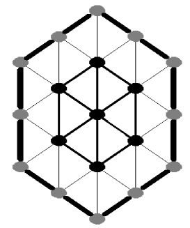
Figure 1: Schematic representation of a cylindrical nanowire (top view). The gray/black circles represents of the surface/shell magnetic atoms, respectively

The Hamiltonian of the nanowire is given by

$$\mathcal{H}=-J_{1}{{\underset{<i,j>}{\overset{}{\displaystyle\sum}}}s_{i}s_{j}}-J_{2}{{\underset{<m,n>}{\overset{}{\displaystyle\sum}}}s_{m}s_{n}}-J_{3}{{\underset{<i,m>}{\overset{}{\displaystyle\sum}}}s_{i}s_{m}}-{{\underset{i}{\overset{}{\displaystyle\sum}}}H_{i}s_{i}}-{{\underset{m}{\overset{}{\displaystyle\sum}}}H_{m}s_{m}}$$ (1)

where $s_{i}$ is the $z$ component of the spin at a lattice site $i$ and it takes the values $s_{i}=\pm 1$ for the spin-1/2 system, $J_{1}$ and $J_{2}$ are the exchange interactions between spins which are located at the core and shell, respectively, and $J_{3}$ is the exchange interaction between the core and shell spins which are nearest neighbor to each other. $H_{i}$ and $H_{m}$ are the external longitudinal magnetic fields at the lattice sites $i$ and $m$ respectively. Magnetic fields are distributed to lattice sites by a given probability distribution. The first three summations in Eq. (1) is over the nearest-neighbor pairs of spins, and the other summations are over all the lattice sites.

This work deals with the following discrete magnetic field distribution, namely trimodal distribution

$$P\left(H_{i}\right)=p\delta\left(H_{i}\right)+\frac{1-p}{2}\left[\delta\left(H_{i}-H_{0}\right)+\delta\left(H_{i}+H_{0}\right)\right]$$ (2)

which covers a bimodal distribution for $p=0$ and reduces to the system with zero magnetic field (pure system) for $p=1$. According to the distribution given in Eq. (2), $p$ percentage of the lattice sites are subjected to a magnetic field $H_{i}=0$, while half of the remaining sites are under the influence of a field $H_{i}=H_{0}$ whereas the field $H_{i}=-H_{0}$ acts on the remaining sites.

We have to separate four representative spins according to their interactions with other spins. Their magnetizations ($m_{i},i=1,2,3,4$) can be given by usual EFT equations which are obtained by differential operator technique and decoupling approximation (DA) [45, 46],

$$\begin{array}[]{lcl}m_{1}&=&\left[A_{1}+m_{1}B_{1}\right]^{4}\left[A_{3}+m_{2}B_{3}\right]\left[A_{3}+m_{3}B_{3}\right]^{2}\left[A_{1}+m_{4}B_{1}\right]\\ m_{2}&=&\left[A_{3}+m_{1}B_{3}\right]\left[A_{2}+m_{2}B_{2}\right]^{2}\left[A_{2}+m_{3}B_{2}\right]^{2}\\ m_{3}&=&\left[A_{3}+m_{1}B_{3}\right]^{2}\left[A_{2}+m_{2}B_{2}\right]^{2}\left[A_{2}+m_{3}B_{2}\right]^{2}\\ m_{4}&=&\left[A_{1}+m_{1}B_{1}\right]^{6}\left[A_{1}+m_{4}B_{1}\right]^{2}\\ \end{array}$$ (3)

Here $m_{1},m_{4}$ are the magnetizations of the two different representative sites in the core and $m_{2},m_{3}$ are the magnetizations of the two different representative sites in the shell. The coefficients in Eq. (3) are

$$\begin{array}[]{lcl}A_{n}&=&\cosh\left(J_{n}\nabla\right)F\left(x\right)|_{x=0}\\ B_{n}&=&\sinh\left(J_{n}\nabla\right)F\left(x\right)|_{x=0}\\ \end{array}$$ (4)

where $\nabla$ is the usual differential operator in the differential operator technique and $n=1,2,3$. The function is defined by

$$F\left(x\right)={{\underset{}{\overset{}{\displaystyle\int}}}}dH_{i}P\left(H_{i}\right)f\left(H_{i},x\right)$$ (5)

where

$$f\left(H_{i},x\right)=\tanh\left(\beta x+\beta H_{i}\right).$$ (6)

In Eq. (6), $\beta=1/(k_{B}T)$ where $k_{B}$ is Boltzmann constant and $T$ is the temperature. The effect of the exponential differential operator to a function is given by

$$\exp{\left(a\nabla\right)}F\left(x\right)=F\left(x+a\right)$$ (7)

with any constant $a$. DA will give the results of the Zernike approximation [47] for this system.

With the help of the Binomial expansion, Eq. (3) can be written in the form

$$\begin{array}[]{lcl}m_{1}&=&{{\underset{i=0}{\overset{4}{\displaystyle\sum}}}}{{\underset{j=0}{\overset{1}{\displaystyle\sum}}}}{{\underset{k=0}{\overset{2}{\displaystyle\sum}}}}{{\underset{l=0}{\overset{1}{\displaystyle\sum}}}}K_{1}\left(i,j,k,l\right)m_{1}^{i}m_{2}^{j}m_{3}^{k}m_{4}^{l}\\ m_{2}&=&{{\underset{i=0}{\overset{1}{\displaystyle\sum}}}}{{\underset{j=0}{\overset{2}{\displaystyle\sum}}}}{{\underset{k=0}{\overset{2}{\displaystyle\sum}}}}K_{2}\left(i,j,k\right)m_{1}^{i}m_{2}^{j}m_{3}^{k}\\ m_{3}&=&{{\underset{i=0}{\overset{2}{\displaystyle\sum}}}}{{\underset{j=0}{\overset{2}{\displaystyle\sum}}}}{{\underset{k=0}{\overset{2}{\displaystyle\sum}}}}K_{3}\left(i,j,k\right)m_{1}^{i}m_{2}^{j}m_{3}^{k}\\ m_{4}&=&{{\underset{i=0}{\overset{6}{\displaystyle\sum}}}}{{\underset{l=0}{\overset{2}{\displaystyle\sum}}}}K_{4}\left(i,l\right)m_{1}^{i}m_{4}^{l}\\ \end{array}$$ (8)

where

$$\begin{array}[]{lcl}K_{1}\left(i,j,k,l\right)&=&\left(\begin{array}[]{c}4\\ i\end{array}\right)\left(\begin{array}[]{c}1\\ j\end{array}\right)\left(\begin{array}[]{c}2\\ k\end{array}\right)\left(\begin{array}[]{c}1\\ l\end{array}\right)A_{1}^{5-i-l}A_{3}^{3-j-k}B_{1}^{i+l}B_{3}^{j+k}\\ K_{2}\left(i,j,k\right)&=&\left(\begin{array}[]{c}1\\ i\end{array}\right)\left(\begin{array}[]{c}2\\ j\end{array}\right)\left(\begin{array}[]{c}2\\ k\end{array}\right)A_{2}^{4-j-k}A_{3}^{1-i}B_{2}^{j+k}B_{3}^{i}\\ K_{3}\left(i,j,k\right)&=&\left(\begin{array}[]{c}2\\ i\end{array}\right)\left(\begin{array}[]{c}2\\ j\end{array}\right)\left(\begin{array}[]{c}2\\ k\end{array}\right)A_{2}^{4-j-k}A_{3}^{2-i}B_{2}^{j+k}B_{3}^{i}\\ K_{4}\left(i,l\right)&=&\left(\begin{array}[]{c}6\\ i\end{array}\right)\left(\begin{array}[]{c}2\\ l\end{array}\right)A_{1}^{8-i-l}B_{1}^{i+l}\\ \end{array}$$ (9)

These coefficients can be calculated from the definitions given in Eqs. (4) and (7).

For a given Hamiltonian and field distribution parameters, by determining the coefficients from Eq. (9) we can obtain a system of coupled non linear equations from Eq. (8), and by solving this system we can get the magnetizations $m_{i},i=1,2,3,4$. The magnetization of the core $(m_{c})$ and shell $(m_{s})$ of nanowire, as well as the total magnetization $(m_{T})$ can be calculated via

$$m_{c}=\frac{1}{7}\left(6m_{1}+m_{4}\right),\quad m_{s}=\frac{1}{12}\left(6m_{2}+6m_{3}\right),\quad m_{T}=\frac{1}{19}\left(6m_{1}+6m_{2}+6m_{3}+m_{4}\right)$$ (10)

Since in the vicinity of the critical point all magnetizations are close to zero, we can obtain another coupled equation system for determining this critical point by linearizing the equation system given in Eq. (8), i.e.

$$A.m=0$$ (11)

where

$$A=\left(\begin{array}[]{cccc}K_{1}(1,0,0,0)&K_{1}(0,1,0,0)&K_{1}(0,0,1,0)&K_{1}(0,0,0,1)\\ K_{2}(1,0,0)&K_{2}(0,1,0)&K_{2}(0,0,1)&0\\ K_{3}(1,0,0)&K_{3}(0,1,0)&K_{3}(0,0,1)&0\\ K_{4}(1,0)&0&0&K_{4}(0,1)\\ \end{array}\right)$$ (12)

$$m=\left(\begin{array}[]{c}m_{1}\\ m_{2}\\ m_{3}\\ m_{4}\\ \end{array}\right)$$ (13)

Critical temperature can be determined from $det(A)=0$. As discussed in [33], the matrix $A$ given in Eq. (12) is invariant under the transformation $J_{3}\rightarrow-J_{3}$ then we can conclude that the system with ferromagnetic ($J_{3}>0$) core-shell interaction has the same critical temperature as that of the system with anti-ferromagnetic ($J_{3}<0$) core-shell interaction (with the same $|J_{3}|$) for certain Hamiltonian and magnetic field distribution parameters. Although this discussion has been made for the system with zero magnetic field in [33], this conclusion is also valid for this system, because of the symmetry of the magnetic field distribution. The equation $det(A)=0$ is invariant under the transformation $J_{3}\rightarrow-J_{3}$ for the nanowire with trimodal magnetic field distribution.

4 Results and Discussion

In this work we discuss the effect of the random magnetic field distribution on the phase diagrams of the system. Since the phase diagrams are the same for the $J_{3}>0$ and $J_{3}<0$ with the same $|J_{3}|$, we focus ourselves on the case $J_{3}>0$, i.e ferromagnetic core-shell interaction. We use the scaled interactions as

$$J_{1}=J,\quad r_{n}=\frac{J_{n}}{J},\quad n=2,3.$$ (14)

Let us start with bimodal magnetic field distribution.

4.1 Bimodal Distribution

This distribution is given by Eq. (2) with $p=0$. It is a well known fact that, in this distribution, increasing $H_{0}$ values drag the system to the disordered phase, due to the random distribution of the magnetic fields $\pm H_{0}$ on the lattice sites. On the other hand, the interactions $J_{n},(n=1,2,3)$ enforce the system to stay in the ordered phase. Thus a competition takes place between these two factors, in addition to the thermal agitations.

The phase diagrams in $(k_{B}T_{c}/J,H_{0}/J)$ plane can be seen in Fig. 2 for different $r_{2}$ and $r_{3}$ values. We can see from Fig. 2 that the general effect of increasing $H_{0}$ is to decrease the critical temperature, as expected. Besides, another expected result is that the higher $r_{2}$ or $r_{3}$ values has the higher $T_{c}$ values at a certain $H_{0}$ value which can be seen in Fig. 2. But we can see in Fig. 2(a) that, the latter observation does not hold for $r_{3}=0$ case. In the absence of the interface interaction between the core and shell, the phase diagrams in $(k_{B}T_{c}/J,H_{0}/J)$ plane are the same for all $r_{2}\leq r_{2}^{\star}$ values. In order to clarify this situation, we plot the curves of the core magnetization, shell magnetization and the total magnetization of the system in Fig. 3. As seen in Fig. 3, shell magnetization falls to zero at a temperature lower than that of the core for the $r_{2}=0.8,1.0$. For these values, the core determines the critical temperature of the system. But for the value of $r_{2}=2.0$, the critical temperature of the shell is higher than the critical temperature of the core. Then we can say that shell of the nanowire has a lower critical temperature than that of the core, up to a certain $r_{2}=r_{2}^{\star}$ value, after that $r_{2}^{\star}$ value, the critical temperature of the shell becomes higher than the critical temperature of the core i.e. the shell begins to determine the critical temperature of the system. This means that for the values that satisfies $r_{2}<r_{2}^{\star}$, the phase diagram of the system does not affected by the changing $r_{2}$. Although the $r_{2}=1.5$ curve in Fig. 2(a) is different from other $r_{2}$ curves corresponding to $r_{2}<1.5$ for the higher $H_{0}/J$ (which are close to the $H_{0}/J=3.0$) values, we can say that this $r_{2}^{\star}$ value satisfies $r_{2}>1.0$. This fact can be explained by taking a look at the geometry of the system. In the absence of the interaction between the core and shell, both of the two distinct shell spins have four nearest neighbors (which have magnetizations labeled as $m_{2},m_{3}$) and the two distinct core spins have five and eight nearest neighbors, respectively (which have magnetizations labeled as $m_{1},m_{4}$). Thus we can say that for equal exchange interactions of the core and shell ($r_{2}=1$), the core has higher critical temperature than that of the shell. Consequently, $r_{2}$ value that providing the equality of the critical temperatures of the core and shell has to be $r_{2}>1.0$. In summary, we can conclude that, for the $r_{3}=0$ phase diagrams in $(k_{B}T_{c}/J,H_{0}/J)$ plane, all diagrams are the same up to a certain $r_{2}^{\star}>1.0$ value, and when $r_{2}=r_{2}^{\star}$, the diagrams begin to separate from the diagrams which are for the $r_{2}<r_{2}^{\star}$ in the higher $H_{0}/J$ region. Furthermore, as $r_{2}$ grows then the phase diagrams become completely separate from the diagrams for the $r_{2}<r_{2}^{\star}$.

We can see from Fig. 2 that, increasing $r_{2}$ and $r_{3}$ values make the ferromagnetic region wider in ($k_{B}T_{c}/J,H_{0}/J$) plane, since increasing $r_{2}$ and $r_{3}$ values rises the absolute value of the lattice energy coming from the spin-spin interaction, which must be overcomed by both thermal agitations and random magnetic fields for the phase transition from an ordered phase to a disordered one.

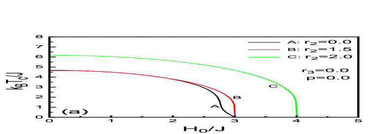
Figure 2: The phase diagrams of the nanowire with bimodal random field distribution in the ($k_{B}T_{c}/J,H_{0}/J)$ plane for different $r_{2},r_{3}$ values.

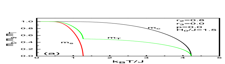
Figure 3: Variation of the magnetization with temperature for some selected $r_{2}$ parameter value of the nanowire with bimodal random field distribution. Fixed parameter values are $r_{3}=0.0,H_{0}/J=1.5$.

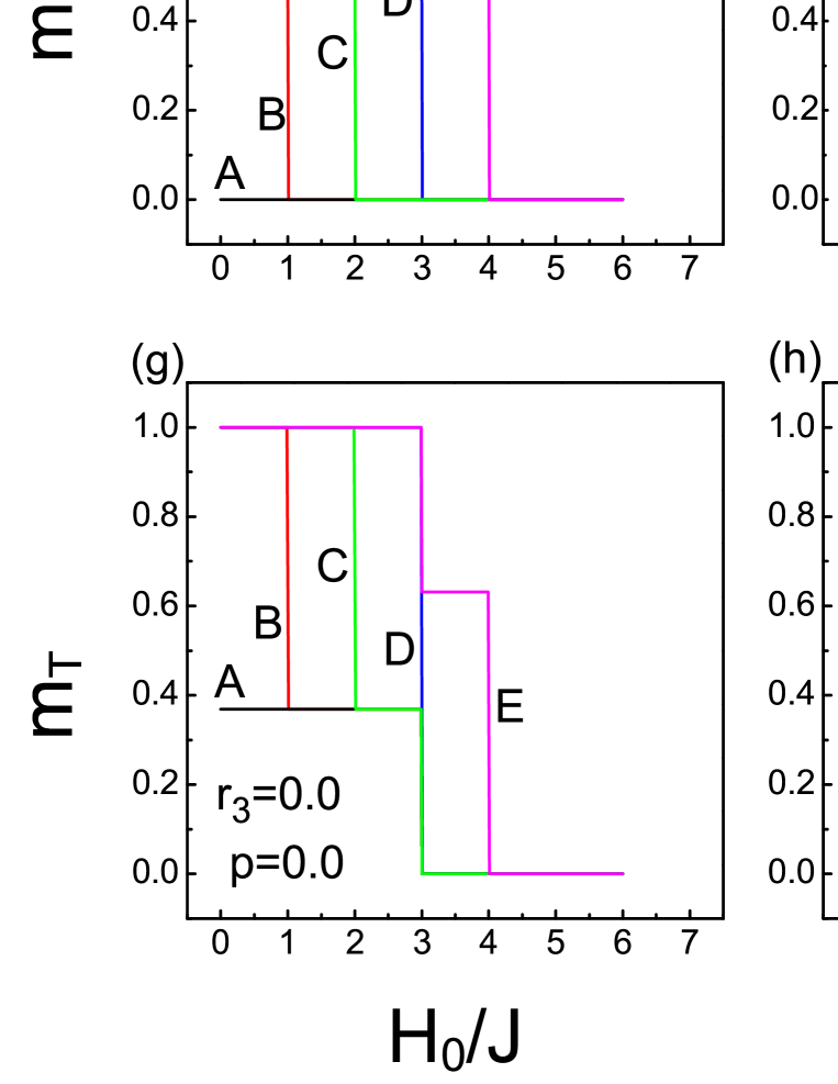
Figure 4: Variation of the ground state magnetizations with $H_{0}/J$ which corresponds to the phase diagrams seen in Fig. 2 for the system with bimodal magnetic field distribution. Each magnetization calculated at a temperature $k_{B}T/J=0.001$ which can be regarded as ground state. The letters which are close to the related curve represent the different $r_{2}$ values as (A) $r_{2}=0.0$, (B) $r_{2}=0.5$, (C) $r_{2}=1.0$, (D) $r_{2}=1.5$, (E) $r_{2}=2.0$

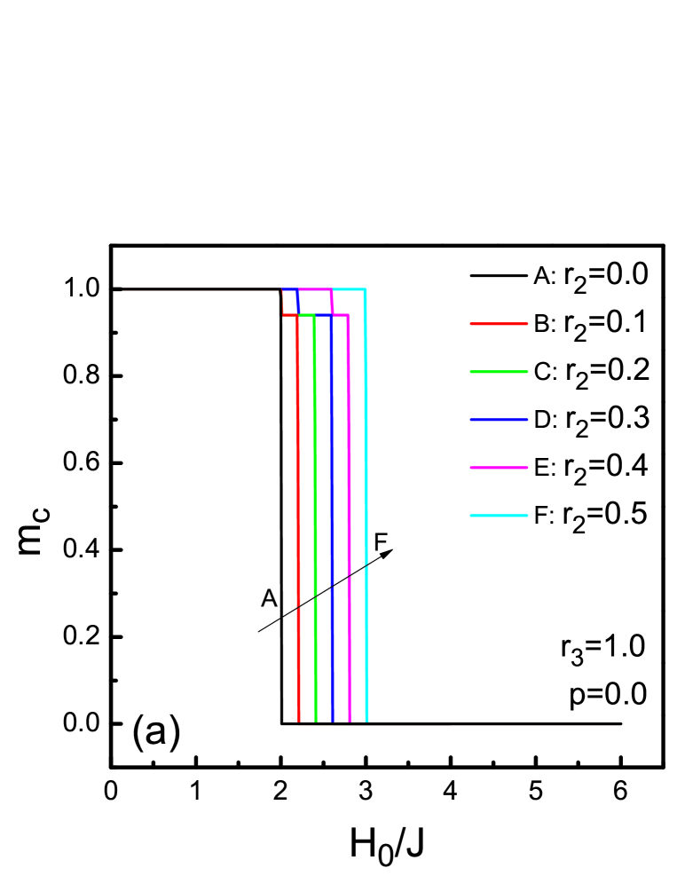
Figure 5: Variation of the ground state magnetizations for selected values of $r_{2}$ for the system with bimodal magnetic field distribution. Each magnetization calculated at a temperature $k_{B}T/J=0.001$ which can be regarded as ground state and for the parameter value $r_{3}=1.0$.

Now the question is: what is the magnetization behavior for that different $r_{2},r_{3}$ and $H_{0}$ values for bimodal magnetic field distribution. Since the magnetization behavior with temperature is well known for the nanowire without any random magnetic field and due to the number of parameters in this problem and also the restrictions on the length of the paper, we restrict ourselves to this question: what is the ground state magnetization behaviors with $H_{0}$ form different $r_{2},r_{3}$ values? We can see the answer of the question from Fig. 4 which is the variation of the core ground state magnetization($m_{c}^{g}$), shell ground state magnetization ($m_{s}^{g}$) and the total ground state magnetization ($m_{T}^{g}$) (where the superscript $g$ stands for the ground state) with $H_{0}$. This figure corresponds to the phase diagrams given in Fig. 2 and the temperature is chosen as $k_{B}T/J=0.001$ which can be regarded as ground state for the system. As seen in Fig. 4(g), in the absence of the core-shell interaction (i.e. $r_{3}=0$), two more ground state magnetization appears apart from the magnetizations $m_{T}^{g}=0.0$ and $m_{T}^{g}=1.0$ which are correspond to the disordered state and ordered state, respectively. These two more ground state magnetization values are $m_{T}^{g}=0.3684$ and $m_{T}^{g}=0.6316$ and can be regarded as two different partially ordered phases of the nanowire under the bimodal magnetic field distribution. Since the core has the ground state magnetization $m_{c}^{g}=1.0$ regardless of the value of $r_{2}$ up to the value of $H_{0}/J=3.0$ ( Fig. 4(a)), that partially ordered phases seen in Fig. 4(g) has to come from the mismatch in magnetization behaviors with $H_{0}$ in the core and shell. It can be seen from Eq. (10) that the core contributes to the total magnetization with the ratio $7/19$ while this ratio for the shell is $12/19$. Because of the difference of the regions which are core and shell in ordered and disordered phases with $H_{0}$, this two partially ordered phases appears in the regions seen in Fig. 4(g). For example, for the $r_{3}=0.0,r_{2}=2.0$, the core has ground state magnetization $m_{c}^{g}=1.0$ up to $H_{0}/J=3.0$ and the shell has ground state magnetization $m_{s}^{g}=1.0$ up to $H_{0}/J=4.0$ then a partially ordered phase $m_{T}^{g}=0.6316=12/19$ appears in the intersection of this two region which is $3.0<H_{0}/J<4.0$.

The presence of the interaction between the core and shell makes this situation slightly different. When $r_{3}\neq 0.0$ then the system becomes whole instead of separate core and shell as in the case $r_{3}=0.0$. Then the core and the shell can develop partially ordered phases separately, thus new partially ordered phases can appear in the system. As seen in Fig. 4(e), shell can develop two new partially ordered phases (other than phases that corresponds to ordered $m_{s}^{g}=1.0$ and disordered $m_{s}^{g}=0.0$ phases) which have magnetizations $m_{s}^{g}=0.5$ ($r_{2}=0$) and $m_{s}^{g}=0.9835$ ($r_{2}=0.5,1.0$) due to the random field and presence of the interaction with the core. This makes the ground state magnetization of the system as in Fig. 4(h) with the same reasoning explained just above, with two partially ordered phases namely $m_{T}^{g}=0.6842$ ($r_{2}=0$) and $m_{T}^{g}=0.9896$ ($r_{2}=0.5,1.0$). The increasing interaction strength between the core and shell increases the magnetization of that two partially ordered phases that has magnetization near to $1.0$ of the shell and then the ground state magnetizations of the system become as seen in Fig. 4(i).

More detailed investigation on that partially ordered phases can show that, indeed a few other partially ordered phases exist in the shell even in the core. This fact can be seen in Fig. 5. As in Fig. 5(a) for $r_{3}=1.0$, with little $r_{2}$ (e.g. $r_{2}=0.3$), rising $H_{0}$ can induce a partially ordered phase in the core which disappears with rising $r_{2}$ (e.g. $r_{2}=0.5$). The same thing also be valid for the shell as seen in Fig. 5(b) and thus whole system which can be seen in Fig. 5(c).

4.2 Trimodal Distribution

Let us investigate the phase diagrams in the ($k_{B}T_{c}/J,H_{0}/J$) plane for the distribution which is given by Eq. (2) for the $p\neq 0$. We can see from the random magnetic field distribution that, when $p$ approaches to $p=1$ from the value $p=0$, the phase diagrams given in Fig. 2 have to evolve to the phase diagrams of the system with zero magnetic field, i.e. parallel lines to the $H_{0}/J$ axes in that plane. This evolution can be seen in Fig. 6. We can see from the Fig. 6 that (e.g. $r_{2}=1.0,r_{3}=1.0$ curve in order of Fig. 6 (a),(c),(e),(g)) , rising $p$ from the $p=0$ to the $p=1$ first opens phase diagrams on the right hand sides of them, then creates a tail on that side which extends to the high magnetic fields then rises that tail to the level of the pure system’s critical temperature. The same effect can be also performed by the rising $r_{2}$ (or $r_{3}$) in the trimodal distribution for little $p$ values, since that effect results from the competition between the spin-spin interaction which tends system to ordered phase and randomly distributed magnetic field. This can be seen for instance in Fig. 6(c). We also note that, during this evolution process a phenomena called reentrant can be seen in the diagrams.

The details of the evolution process of the phase diagram with $p$ in the ($k_{B}T_{c}/J,H_{0}/J$) plane for fixed $r_{2}=1.0,r_{3}=1.0$ values can be seen in Fig. 7. We can see from Fig. 7 that, at zero temperature the transitions from the ordered phase to a disordered one occurs at integer $H_{0}/J$ values.

The ground state magnetizations appear more complicated forms for this distribution than the bimodal distribution. This can be seen from Fig. 8 which are corresponding ground state magnetizations to the phase diagrams given in Fig. 6(a),(c),(e),(g). Construction of the total ground state magnetization from the ground state magnetizations of the core and shell is the same as explained in the bimodal distribution section, since trimodal distribution does not change the contribution ratios of the core and shell to the total magnetization. But we can see from Fig. 8 that, trimodal distribution induce higher number of partially ordered phases to the system both core and shell than the bimodal distribution. This causes higher number of partially ordered phases of the whole system. It is not meaningful to give all the ground state magnetization values of that ordered phases seen in Fig. 8, since that values depends on the parameters $r_{2},r_{3},p$ and $H_{0}$. But we have to say that rising $r_{2}$ for fixed $r_{3}=1.0$, shifts the partially ordered phases to the right of the $m_{T}-H_{0}/J$ plane, means that increasing $r_{2}$ destroys partially ordered phases with beginning in low $H_{0}/J$. We can also see from Fig. 8 that the same effect can be done by rising $p$, i.e. also rising $p$ destroys the partially ordered phases beginning from the low $H_{0}/J$. Thus we can say that rising $r_{2}$ for other fixed parameters or rising $p$ for other fixed parameters induces same changes on both phase diagrams and the ground state magnetizations. This similarity is expected because rising $r_{2}$ means that interactions between spins in the shell getting stronger, then after some value of $r_{2}$ this interactions can overcome the effect of the random magnetic field distribution. On the other hand rising $p$ means that the falling strength of the randomness, then system can escape from that partially ordered phases which are formed by randomness effects.

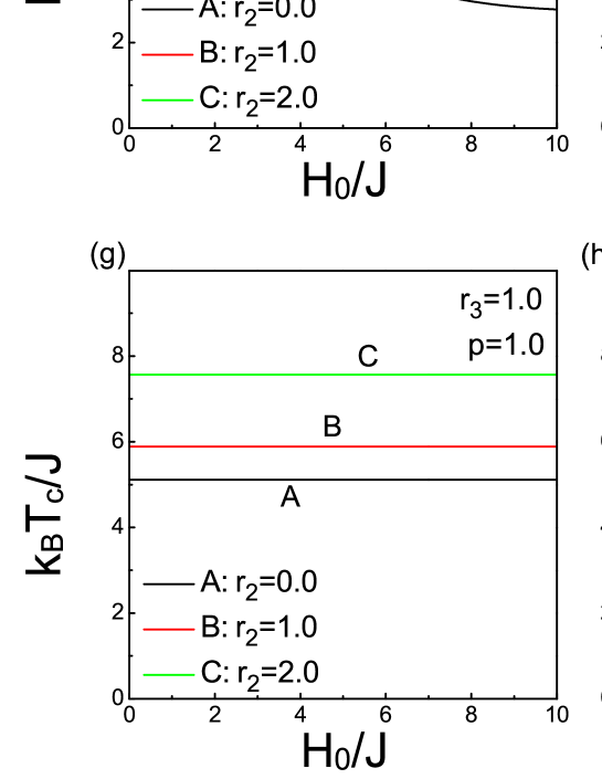
Figure 6: The phase diagrams of the nanowire with trimodal random field distribution in the $(k_{B}T_{c}/J,H_{0}/J)$ plane for different $r_{2},r_{3},p$ values

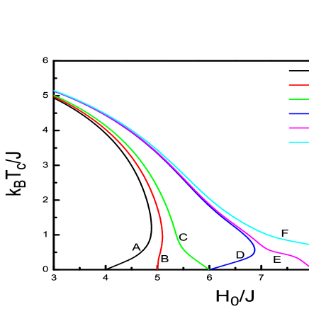
Figure 7: The phase diagrams of the nanowire with trimodal random field distribution in the $(k_{B}T_{c}/J,H_{0}/J)$ plane for different $p$ values. Fixed values of the diagrams are $r_{2}=1.0$ and $r_{3}=1.0$.

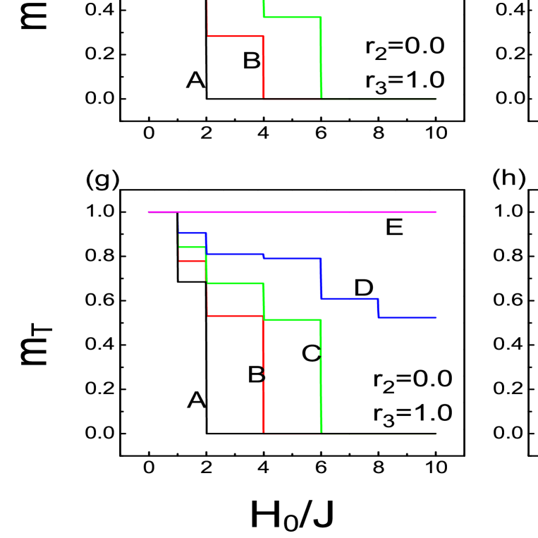
Figure 8: Variation of the ground state magnetizations for selected values of $r_{2}$ and $p$ for the system with trimodal magnetic field distribution. Each magnetization calculated at a temperature $k_{B}T/J=0.001$ which can be regarded as ground state and for the parameter value $r_{3}=1.0$. The letters which are close to the related curve represent the different $p$ values as (A) $p=0.0$, (B) $p=0.3$, (C) $p=0.5$, (D) $p=0.7$, (E) $p=1.0$

5 Conclusion

The effect of the random magnetic field distribution on the phase diagrams and ground state magnetizations of the Ising nanowire investigated. The evolution of the phase diagrams of the system with bimodal magnetic field distribution to the pure one (i.e. system with no magnetic field) investigated as the distribution parameter of the magnetic field goes from $p=0$ to $p=1$. In the bimodal distribution as a special case of the trimodal distribution with $p=0$, some partially ordered phases seen for the system as a result of the inspection of the ground state magnetizations. This complicated situation in the ground state magnetizations comes from the competition between the randomness of the magnetic field which drag the system to the disordered phase and the interaction strengths between the spins which try to hold the system in an ordered phase.

Our findings about the phase diagrams in $(k_{B}T_{c}/J-H_{0}/J)$ plane as follows:

• All closed phase diagrams intersect $H_{0}/J$ axes at integer $H_{0}/J$ values. This means that at zero temperature, system has ferromagnetic ordering up to the some value of $H_{0}$ which is multiple of the core interaction strength $J$.

• In the absence of the core-shell interaction ($r_{3}=0.0$) the phase diagrams for different $r_{2}$ values are the same up to some $r_{2}<r_{2}^{\star}$ value where $r_{2}^{\star}>1.0$ for the bimodal distribution. This fact comes from the difference between the total interaction energy of the core and shell. When $r_{2}$ reaches the value $r_{2}^{\star}$, shell starts to determine the critical temperature of the system and thus phase diagrams for $r_{2}>r_{2}^{\star}$ become separate.

• Phase diagrams of the system with trimodal magnetic field distribution getting open on the high $H_{0}/J$ region when $p$ is sufficiently large. This is due to the decreasing randomness.

Lastly our findings about the ground state magnetization values as follows:

• System with bimodal magnetic field distribution have a few partially ordered phases.

• This number of partially ordered phases getting higher in the trimodal distribution.

• Rising $p$ and also rising $r_{2}$ or $r_{3}$ destroys this partially ordered phases.

These partially ordered phases requires more detailed investigation in order to obtain more precise relations of the numerical values of that ground state magnetizations and the length of a certain ground state magnetization in the $(m-H_{0}/J)$ plane, with random magnetic field distribution parameters. At the same time these partially ordered phases means that, the phase diagrams in $(k_{B}T_{c}/j-H_{0}/J)$ plane have some first order transition lines. But since one can not calculate the free energy of the system within this formulation, we can not explicitly determine these first order transition lines.

Altough these questions waiting for being answered, another important question is the effect of the continuous random magnetic field distributions (e.g. Gaussian distribution) to the phase diagrams of the Ising nanowire. This will be our next work. We hope that the results obtained in this work may be beneficial form both theoretical and experimental point of view.

References

- [1] M. Ruhrig, B. Khamsehpour, K. J. Kirk, J. N. Chapman, P. Aitchison, S. McVitie, and C. D. W. Wilkinsons,IEEE Trans. Magn. 32, 4452 (1996).
- [2] Th. Schrefl, J. Filder, K. J. Kirk, and J. N. Chapman, IEEE Trans. Magn. 33, 4128 (1997).
- [3] Th. Schrefl, J. Filder, K. J. Kirk, and J. N. Chapman, J. Magn. Magn. Mater. 175,193(1997).
- [4] B. Martinez, X. Obradors, L. Balcells, A. Rouanet, and C. Monty, Phys. Rev. Lett. 80, 181 (1998).
- [5] G. V. Kurlyandskaya, M. L. Sanchez, B. Hernando, V. M. Prida, P. Gorria, M. Tejedor, Appl. Phys. Lett. 82 (2003) 3053.
- [6] H. Zeng, J. Li, J. P. Liu, Z. L. Wang, S. Sun, Nature 420 (2002) 395.
- [7] C. Alexiou, A. Schmidt, R. Klein, P. Hullin, C. Bergemann, W. Arnold, J. Magn. Magn. Mater. 252 (2002) 363.
- [8] R. Skomski, J. Phys. :Condens. Matter 15 (2003) R841.
- [9] H. Schlorb, V. Haehnel, M. S. Khatri, A. Srivastav, A. Kumar, L. Schultz, S. Fahler, Phys. Status Solidi B 247 (2010) 2364.
- [10] J. E. Wegrowe, D. Kelly, Y. Jaccard, Ph. Guittienne, J. P. hAnsermet, Europh Lett. 45 (1999) 626.
- [11] A. Fert,L. Piraux, J. Magn. Magn. Mater. 200 (1999) 338.
- [12] R. H. Kodama, J. Magn. Magn. Mater. 200 (1999) 359.
- [13] S. J. Son, J. Reichet, B. He, M. Schuchman, and S. B. Lee, J. Am. Chem. Soc. 127, 7316 (2005).
- [14] D. Lee, R. E. Cohen, and M. F. Rubner, Langmuir 23, 123 (2007).
- [15] A. Hultgren, M. Tanase, C. S. Chen, D. H. Reich, IEEE Transactions on Magnetics 40 (2004) 2988.
- [16] A. Hultgren, M. Tanase, E. J. Felton, K. Bhadriraju, A. K. Salem, C. S. Chen, D. H. Reich, Biotechnology Progress 21 (2005) 509.
- [17] A. F. Bakuzis and P. C. Morais, J. Magn. Magn. Mater. 285, 145 (2005).
- [18] V. S. Leite and W. Figueiredo, Physica A 350, 379 (2005).
- [19] T. Kaneyoshi, Phys. Status Solidi B 242, 2938 (2005).
- [20] T. Kaneyoshi, J. Magn. Magn. Mater. 321, 3430 (2009).
- [21] T. Kaneyoshi, Solid State Commun. 152 (2012) 883
- [22] A. Zaim, M. Kerouad, and Y. El. Amraoui, J. Magn. Magn. Mater. 321, 1077 (2009).
- [23] J. T. Ou, W. Lai, D. L. Lin, and F. Lee, J. Phys. :Condens. Matter 9, 3687 (1997)
- [24] Huaiyu Wang, Yunsong Zhou, D. L. Lin, and Enge Wang, Chin. J. Phys. 39, 85 (2001).
- [25] Huaiyu Wang, Yunsong Zhou, D. L. Lin, and Chongyu Wang, Phys. Stat. Sol. (b) 232, 254 (2002).
- [26] Y. C. Su, R. Skomski, K. D. Sorge, D. J. Sellmyer, Appl. Phys. Lett. 84 (2004) 1525.
- [27] T. Kaneyoshi, J. Magn. Magn. Mater. 322, 3014 (2010).
- [28] T. Kaneyoshi, J. Magn. Magn. Mater. 322, 3410 (2010).
- [29] T. Kaneyoshi, Phys. Status Solidi B 248, 250 (2011).
- [30] T. Kaneyoshi, Solid State Commun. 151 (2011) 1528.
- [31] E. Konstantinova, J. Magn. Magn. Mater. 320, 2721 (2008).
- [32] T. Kaneyoshi, J. Magn. Magn. Mater. 323, 1145 (2011).
- [33] T. Kaneyoshi, J. Magn. Magn. Mater. 323, 2483 (2011).
- [34] T. Kaneyoshi, Physica A 390, 3697 (2011).
- [35] M. Keskin, N. Sarli, B. Deviren, Solid State Commun. 151 (2011) 1025.
- [36] S. Bouhou, I. Essaoudi, A. Ainane, M. Saber, F. Dujardin, J. J. de Miguel, J. Magn. Magn. Mater. 324 (2012) 2434
- [37] O. Canko, A. Erdinç, F. Taþkin, M. Atýþ, Phys. Lett. A 375 (2011) 3547
- [38] N. Sarli, M. Keskin, Solid State Commun. 152 (2012) 354.
- [39] Y. Yüksel, E. Aydiner, H. Polat, J. Magn. Magn. Mater. 323 (2011) 33168.
- [40] O. Canko, A. Erdinç, F. Taþkin, A. F. Yýldýrým, J. Magn. Magn. Mater. 324 (2012) 508
- [41] A. I. Larkin, Sov. Phys. JETP 31, 784 (1970).
- [42] Y. Imry and S. K. Ma, Phys. Rev. Lett. 35, 1399 (1975).
- [43] S. Fishman and A. Aharony, J. Phys. C 12, L729 (1979).
- [44] J. L. Cardy, Phys. Rev. B 29, 505 (1984).
- [45] R. Honmura, T. Kaneyoshi, J. Phys. C 12 (1979) 3979.
- [46] T. Kaneyoshi, Acta Phys. Pol. A 83 (1993) 703.
- [47] F. Zernike, Physica 7 (1940) 565.