Collider Signatures of the $N=3$ Lee-Wick Standard Model

Abstract

Inspired by the Lee-Wick higher-derivative approach to quantum field theory, Grinstein, O’Connell, and Wise have illustrated the utility of introducing into the Standard Model negative-norm states that cancel quadratic divergences in loop diagrams, thus posing a potential resolution of the hierarchy problem. Subsequent work has shown that consistency with electroweak precision parameters requires many of the partner states to be too massive to be detected at the LHC. We consider the phenomenology of a yet-higher derivative theory that exhibits three poles in its bare propagators (hence $N=3$), whose states alternate in norm. We examine the interference effects of $W$ boson partners on LHC scattering cross sections, and find that the $N=3$ LWSM already makes verifiable predictions at 10 fb^-1 of integrated luminosity.

I Introduction

Previous work by Grinstein, O’Connell, and Wise Grinstein:2007mp , repurposing the seminal work of Lee and Wick (LW) Lee:1970iw , has demonstrated the effectiveness of introducing negative-norm states to cancel the quadratic divergences endemic to the Standard Model (SM). In this formulation, the LW states amount to the additional solutions of a higher-derivative (HD) field equation possessing two poles in its Feynman propagator. Starting with

$$\mathcal{L}_{\rm HD}=-\frac{1}{2}\hat{\phi}\,\Box\hat{\phi}-\frac{1}{2M^{2}}\hat{\phi}\,\Box^{2}\hat{\phi}-\frac{1}{2}m^{2}\hat{\phi}^{2}+\mathcal{L}_{\rm int}(\hat{\phi})\,,$$ (1)

one obtains

$$\tilde{D}_{\rm HD}(p)=\frac{i}{p^{2}-m^{2}-p^{4}/M^{2}}\,,$$ (2)

which scales as $-p^{-4}$ at high energies, thereby improving the convergence of Feynman diagrams in the HD formulation of the theory. For $M^{2}\gg m^{2}$, the field $\hat{\phi}$ has poles at $p^{2}\approx m^{2}$ and $p^{2}\approx M^{2}$. As in Ref. Grinstein:2007mp , one can perform an auxiliary field redefinition to split the single field $\hat{\phi}$ into two fields, one of positive and one of negative norm:

$$\tilde{D}_{\rm SM}(p)\approx\frac{i}{p^{2}-m^{2}}\,,\ \ \tilde{D}_{\rm LW}(p)\approx\frac{-i}{p^{2}-M^{2}}\,,$$ (3)

which becomes exact in the limit $m^{2}/M^{2}\rightarrow 0$. It was also shown in Grinstein:2007mp that the heavy LW fields have the interesting property of possessing negative decay widths, a feature that figures prominently in the remainder of this work.

The primary theoretical motivation to study the LWSM is rooted in the resolution of the hierarchy problem provided by higher-derivative Lagrangians. The level of attractiveness of this solution relies upon whether these heavy LW states can be definitively observed at colliders using present experimental capabilities (i.e., the LHC). This line of research was initially conducted in Ref. Rizzo:2007ae , in which the author analyzed, among other processes, $pp\rightarrow W_{i}^{+}+X\rightarrow\ell^{+}+\nu_{\ell}+X$, where $W_{i}^{+}$ refers to either a SM or LW virtual gauge boson, and a LW mass of 1.5 TeV was assumed. However, analyses of electroweak parameters carried out in succession of improvements Alvarez:2008za ; Underwood:2008cr ; Carone:2008bs ; Chivukula:2010nw (by scanning the LW parameter space in Alvarez:2008za ; by including only LW masses for the fields most important for the hierarchy problem Carone:2008bs ; by using not just oblique parameters $S$, $T$, but also the “post-LEP” parameters $W$, $Y$ Underwood:2008cr ; by including bounds from the $Zb\bar{b}$ direct correction Chivukula:2010nw ) reach the consensus conclusion that the LW $W$ mass must be at least $\sim 3$ TeV in order to maintain consistency with current electroweak precision tests (EWPT), and even then only at the price of making LW fermion masses substantially higher (as much as 10 TeV, according to the same references). More generic scenarios, in which all LW particles have comparable masses, have typical bounds of $\gtrsim 7$ TeV, which not only places experimental signals out of reach for the LHC, but also diminishes the value of LW states for providing a natural hierarchy problem resolution. Nevertheless, significant work on the phenomenology of the LWSM at the LHC has been carried out in a number of papers Krauss:2007bz ; Carone:2009nu ; Alvarez:2011ah ; Figy:2011yu .

However, the conventional LW approach studied to date provides only the first nontrivial example in a series of higher-derivative theories with an increasing number $N$ of propagator poles. Naming the original theory $N=1$ and the conventional LW theory $N=2$, one may generate an $N=3$ theory Carone:2008iw , or any higher $N$, each of which resolves the hierarchy problem. In particular, the Lagrangian for the scalar $N=3$ theory reads

$$\mathcal{L}_{N=3}=-\frac{1}{2}\hat{\phi}\,\Box\hat{\phi}-\frac{1}{2M_{2}^{2}}\hat{\phi}\,\Box^{2}\hat{\phi}-\frac{1}{2M_{3}^{4}}\hat{\phi}\,\Box^{3}\hat{\phi}-\frac{1}{2}m^{2}\hat{\phi}^{2}+\mathcal{L}_{\rm int}(\hat{\phi})\,,$$ (4)

which gives rise to the propagator

$$\tilde{D}_{\rm HD}(p)=\frac{i}{p^{2}-m^{2}-p^{4}/M_{2}^{2}+p^{6}/M_{3}^{4}}\,.$$ (5)

For $M_{3}\gg M_{2}\gg m$, this theory exhibits three well-separated poles, in analogy to the $N=2$ case discussed above. However, when one performs successive auxiliary field transformations to the original HD Lagrangian, the new state so obtained is a heavy positive-norm field, with a positive decay width just like its SM partner. Work underway LTprep shows that this crucial alternation of norm provides a substantial cancellation of the complete LW contribution to the EWPT, and therefore significantly relaxes the bounds on the LW masses; however, in anticipation of the results of this detailed analysis, we consider here as a first step whether the LW states themselves are easily discernible in realistic LHC data, and whether they are easily distinguishable from other beyond-SM (BSM) scenarios. This work therefore closely follows the approach of Ref. Rizzo:2007ae , which found the answers to these questions for the LW $W$ to be yes and no, respectively; we, on the other hand, show not only that the two LW $W$ states with generic $\leq 2$ TeV masses are easily visible already with 10 fb^-1 of data, but also that the generic case produces a spectrum distinguishable from that generated by other common BSM scenarios.

The only assumptions essential to this analysis are the $+,-,+$ signature of the states and the $M_{3}>M_{2}>m$ hierarchy of masses. The construction of Ref. Carone:2008iw then shows that one can build a canonically normalized Lagrangian of the form

$$\mathcal{L}=\displaystyle\sum_{i=1}^{N}(-1)^{i+1}\left[-\frac{1}{2}\phi^{(i)}\left(\Box+m_{i}^{2}\right)\phi^{(i)}\right]+\mathcal{L}_{\rm int}(\{\phi^{(i)}\})\,,$$ (6)

where $i=1$ refers to the SM state, $i=2$ refers to the negative-norm LW state, $i=3$ refers to the heavy positive-norm LW state, and so on, up to arbitrary $N$.

This paper is organized as follows: In Sec. II, we outline the method of calculation for analyzing collider production of $W_{i}$ states, and discuss the expected signals of such states from not only LW, but Kaluza-Klein (KK) and other popular BSM scenarios as well. We present our results in Sec. III, which indicate definite LHC discovery potential, and offer conclusions in Sec. IV. Technical details of the calculation are relegated to the Appendix.

II Methods

We are primarily interested in the semileptonic process $pp\rightarrow\ell^{+}+\nu_{\ell}+X$, where the leptons are produced by an intermediate $W_{i}^{+}$, and $X$ is an inclusive hadronic final state. To leading order in weak interactions, one obtains the partonic-level differential cross section Rizzo:2007ae

$$\frac{d^{3}\sigma}{d\tau\;dy\;dz}=K\frac{G_{F}^{2}M_{W}^{4}}{48\pi}\displaystyle\sum_{qq^{\prime}}|V_{qq^{\prime}}|^{2}[SG^{+}_{qq^{\prime}}(1+z^{2})+2AG_{qq^{\prime}}^{-}z],$$ (7)

with the variables defined by

$$S \equiv \displaystyle\sum_{ij}P_{ij}(C_{i}C_{j})^{\ell}(C_{i}C_{j})^{q}(1+h_{i}h_{j})^{2}\,,$$ (8)

$$A \equiv \displaystyle\sum_{ij}P_{ij}(C_{i}C_{j})^{\ell}(C_{i}C_{j})^{q}(h_{i}+h_{j})^{2}\,,$$ (9)

$$P_{ij} \equiv \hat{s}\frac{(\hat{s}-M_{i}^{2})(\hat{s}-M_{j}^{2})+\Gamma_{i}\Gamma_{j}M_{i}M_{j}}{[(\hat{s}-M_{i}^{2})^{2}+\Gamma_{i}^{2}M_{i}^{2}][i\rightarrow j]}\,.$$ (10)

Here, $K$ is a numerical factor $\simeq 1.3$ arising from NLO and NNLO QCD corrections Melnikov:2006kv , and $z\equiv\mathrm{cos}\;\theta^{*}$ is the center-of-momentum (CM) frame scattering angle of parton $q$ into charged lepton $\ell^{+}$. The factors $P_{ij}$ represent cross terms between the allowed $W^{+}_{i}$ propagators (see the Appendix for a detailed description of the calculation of $\Gamma$), and the $S$ (symmetric) and $A$ (antisymmetric) terms are the combinations of helicities $h_{i}$ and couplings $C_{i}^{\ell,q}$ of the leptons and quarks that carry the indicated parities with respect to the variable $z$. The $G_{qq^{\prime}}^{\pm}$ are combinations of parton distribution functions (PDFs) Martin:2009iq :

$$G_{qq^{\prime}}^{\pm}=q(x_{a},\,M^{2})\bar{q}^{\prime}(x_{b},\,M^{2})\pm q(x_{b},\,M^{2})\bar{q}^{\prime}(x_{a},\,M^{2})\,,$$ (11)

where $q$ ($q^{\prime}$) are the PDFs associated with an up (down)-type quark, the lepton invariant mass is $M^{2}\equiv\hat{s}$, and $x_{a,b}=\sqrt{\tau}e^{\pm y}$ are the parton longitudinal momentum fractions, where $\tau\equiv\hat{s}/s$, and $y$ is the virtual gauge boson rapidity. At the level of the differential cross section, the present work extends the calculation of Ref. Rizzo:2007ae by introducing an additional heavy state with positive norm, and hence with $\Gamma_{3}>0$. One converts the differential cross section Eq. (7) into a distribution in the transverse mass $M_{T}$, obtained from $z=(1-M_{T}^{2}/M^{2})^{1/2}$:

$$\frac{d\sigma}{dM_{T}}=\displaystyle\int_{M_{T}^{2}/s}^{1}d\tau\int_{-Y}^{Y}dy\;J(z\rightarrow M_{T})\frac{d^{3}\sigma}{d\tau\;dy\;dz}\,.$$ (12)

The Jacobian factor $J(z\rightarrow M_{T})=|dz/dM_{T}|=\frac{M_{T}}{M^{2}}|1-M_{T}^{2}/M^{2}|^{-1/2}$ produces the peak structures seen in the plots in the next section. The new positive-norm state produces an observable signal in the region near $M_{T}\approx M_{3}$, with a distinctive sharp interference edge generated by the off-diagonal terms in $P_{ij}$.

How do the predictions of the $N=3$ LWSM compare with those of other theories featuring a heavy $W^{\prime}$ boson? The $W^{\prime}$ could, in principle, have arbitrary helicities and couplings to SM fields. The alternating-norm LW states offer just one such example amidst a plethora of possibilities. These include the Sequential Standard Model (the SM with extra gauge bosons carrying the same couplings), left-right symmetric models (such as Pati-Salam), and KK excitations of the $W$ on a compactified $S^{1}/{Z}_{2}$ dimension (see Davoudiasl:2007cy for a thorough list of references). It was shown in Rizzo:2007ae that the first two scenarios are already clearly distinguishable from the $N=2$ LWSM, so we do not consider them further. The hypothetical KK excitations of the $W$, on the other hand, demand a more careful treatment.

The most straightforward universal extra dimension models Barbieri:2004qk already require $R^{-1}$ to exceed several TeV, but alternative mechanisms allow $R^{-1}$ to be brought down to scales that can be probed at the LHC. Suppose, for example, that gauge and Higgs bosons propagate in the bulk of the $S^{1}/Z_{2}$ dimension $y\in[0,\pi R]$, but that leptons are localized at $y=0$ and quarks are localized at $y=\pi R$ ArkaniHamed:1999za . Such a mechanism can have a lower compactification scale; as in Ref. Rizzo:2007ae , for sake of argument we take it to be $R^{-1}\sim 1.5$ TeV. The $n^{\rm th}$ mode of the $W$ in the compactified dimension has a 5D wave function of the form $\cos(ny/R)$. Reading off the couplings from Eq. (3) of Ref. Rizzo:1999br , one sees that the localization of the quarks at $y=\pi R$ forces their couplings in the 4D effective theory to be $C_{n}^{q}=(-1)^{n}$ for the $n^{\rm th}$ KK excitation of the $W$. Upon making this change to Eq. (8), one finds that the KK excitations can mimic the wrong-sign propagator of the LW bosons quite faithfully. The only algebraic difference comes from the negative sign of $\Gamma_{2}$, but due to the very narrow widths under consideration (as calculated in the Appendix), the two models are potentially virtually indistinguishable. This ambiguity could not be resolved within the framework of the $N=2$ LWSM, but we find that the $N=3$ LWSM yields starkly different predictions.

To illustrate this point, consider the mass term of the KK excitations, with $\varphi_{b}$ being the bulk Higgs field with VEV $|\varphi_{b}|$ Rizzo:1999br and $g$ being the 5D gauge coupling:

$$\mathcal{L}_{\rm mass}=\frac{1}{2}\left(\frac{n^{2}}{R^{2}}+2g^{2}|\varphi_{b}|^{2}\right)V_{\mu}^{(n)}V^{(n)\mu}\,.$$ (13)

One sees that the squared masses of the KK excitations obey a specific $n^{2}$ hierarchy; therefore, if the first excitation has a mass equal to that of the $N=2$ $W$ boson, the mass of the second KK excitation is pre-determined by the theory, whereas the masses of LW bosons can in principle assume any positive values. The spacing restriction is especially apparent in the limit $R^{-1}\gg g|\varphi_{b}|$, in which case the KK excitations have equally spaced masses

$$m_{\rm KK}\approx\frac{n}{R}\,.$$ (14)

In order for the KK and $N=3$ LWSM scenarios to be confused, either the experimental sensitivities must be such that only one excitation can be discerned in each case (which reduces to the situation described in Ref. Rizzo:2007ae ), or the spacing of the LW partners matches by unfortunate chance the spectrum given by Eq. (13). In this case, the natural next step would be to look for the KK and LW partners of other particles and examine their mass spectra for further evidence to distinguish the two possibilities. In general, however, we conclude that the generic $N=3$ LWSM makes unique predictions for mass and coupling spectra that cannot be mimicked by well-known alternative $W^{\prime}$ theories.

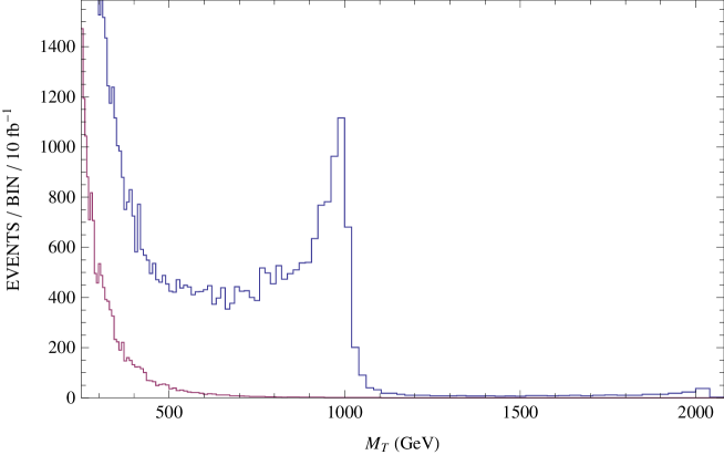
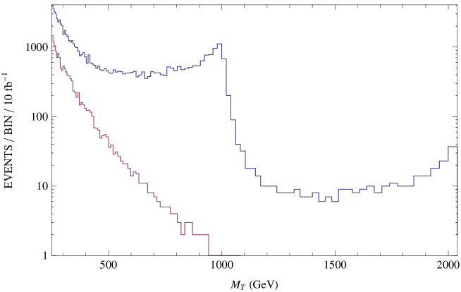
Figure 1: Transverse mass distribution for the $N=3$ LWSM (blue) and expected SM background (red), assuming masses $M_{2}=1$ TeV, $M_{3}=2$ TeV. Both plots display the same data, though the lower plot has a log scale in order to emphasize the second Jacobian peak near the region $M_{T}\approx M_{3}$. We employ a cut $|\eta_{\ell}|<2.5$ on the rapidity of the outgoing leptons, and smear the distribution by $\delta M_{T}/M_{T}\approx 2\%$ to simulate the resolution of the ATLAS detector.

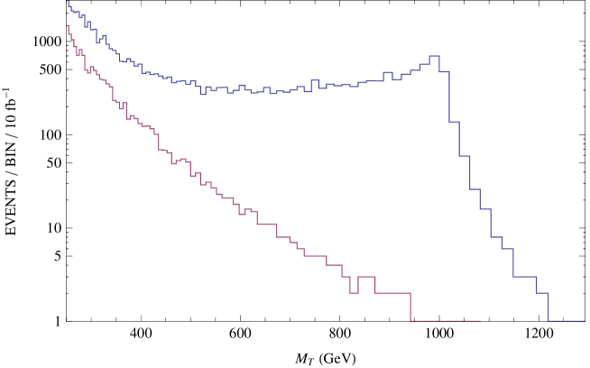
Figure 2: Transverse mass distribution for $M_{2}=1$ TeV, but now $M_{3}=5$ TeV. Even with an integrated luminosity of 10 fb^-1, the second Jacobian peak is too weak to be discernible; the plots are truncated where the simulated number of events per bin drops below 0.5.

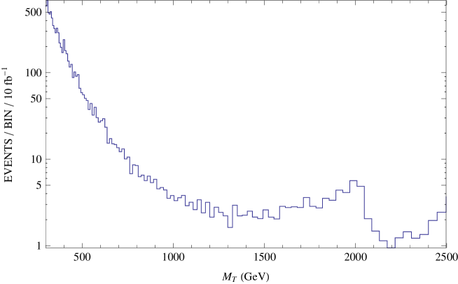
Figure 3: Transverse mass distribution for $M_{2}=2$ TeV, $M_{3}=2.5$ TeV, now at $\sqrt{s}=8$ TeV and an integrated luminosity of 15 fb^-1.

III Results

We start with the LHC inputs $\sqrt{s}=7$ TeV and 10 fb^-1 of integrated luminosity. Assuming the masses $m\approx m_{W,{\rm SM}}=80.4$ GeV, $M_{2}=1$ TeV, $M_{3}=2$ TeV, a set chosen purely for illustration, one then has all the necessary inputs to compute transverse mass distributions in the LWSM. We plot our results in Fig. 1. The most exciting feature is the statistically robust Jacobian peak near $M_{T}\approx M_{3}$ at 10 fb^-1, which is not only revealed as dozens of events that would not appear in the SM or even the $N=2$ LWSM, but one that exhibits a very distinctive morphology. This result indicates that, for a sufficiently light $W_{3}^{\pm}$ boson, the $N=3$ LWSM makes unambiguous predictions (i.e., are highly unlikely to be confused with KK modes or even the $N=2$ LW theory) that can be tested at the LHC, given a reasonable 10 fb^-1 of integrated luminosity. However, we hasten to add that nothing is special about the value $M_{3}=2$ TeV; in principle, the $W_{3}^{\pm}$ could be significantly heavier, still resolving the hierarchy problem (although likely creating tension with EWPT LTprep ), but evading detection any time within the next decade. Behavior that satisfies a theory well can provide a dull phenomenology: A sufficiently heavy $W_{3}^{\pm}$ combined with a lighter $W_{2}^{\pm}$ might still satisfy the EWPT constraints while slipping past the range of detection. Even for $M_{3}=5$ TeV this effect is quite stark; see Fig. 2 for a plot of the transverse mass distribution in such a theory. One can check that the absence of a strong $M_{3}=5$ TeV signal is not due to the limited integrated luminosity, but rather the limited CM energy.

One can also show that a 2012 LHC data set of 15 fb^-1 at $\sqrt{s}=8$ TeV allows the discovery bounds to be pushed even further. In Fig. 3 we present the expectation in such a scenario for $M_{2}=2.0$ TeV and $M_{3}=2.5$ TeV, which provides further evidence that a wide expanse of LW parameter space will be probed in the near future at the LHC. The crucial point of the present work is that, regardless of the masses of the $W_{i}$ under consideration, the alternating-sign metric of the LWSM plus the lack of a specific mass spectrum functional dependence produces distinct Jacobian peak structures that can be easily distinguished from those of other theories.

IV Conclusions

Our work in the $N=3$ LWSM shows that the presence of a heavy, positive-norm state has observable consequences for physics at the LHC. It makes predictions above and beyond that of the conventional $N=2$ LWSM, and moreover is clearly distinguishable from other heavy $W^{\prime}$ theories, most specifically the Kaluza-Klein excitations associated with particles propagating along a compactified $S^{1}/Z_{2}$ dimension. The novel contribution of our work is the second Jacobian peak associated with the $N=3$ $W$ boson. However, since little information exists to constrain the value of $M_{3}$ LTprep , our choice $M_{3}=2$ TeV should be interpreted as one possibility of many. We find that, for a sufficiently heavy choice of $M_{3}$ ($\sim 5$ TeV), the expected signal for the $N=3$ theory does not rise significantly above the SM background for 10 fb^-1 of integrated luminosity.

Finally, one might question the naturalness of the choice $N=3$, and argue either that one has no good reason to stop at 3, or that including as many as 2 LW partners is already excessive. For argument’s sake, why would one settle with a theory of $N$ sets of states when $N+1$ sets might do an even better job of solving the hierarchy problem? It is even possible (albeit unpalatable) for a countably infinite tower of LW states to exist, alternating in the signs of their norms, while still conspiring to cancel out divergences in loop diagrams; the study of field equations of motion for infinite-order propagator poles was addressed in Ref. Pais:1950za , wherein the authors found that basic elements such as the propagator could still be reliably constructed in such a theory. These increasingly heavy states would serve an important theoretical role in the structure of the SM, but would lie far beyond the reach of any collider in the foreseeable future, not to mention creating a proliferation of new degrees of freedom. Moreover, as discussed in the Introduction, the $N=2$ LWSM with lighter partner masses is known to create significant tension with electroweak precision constraints (particularly for custodial isospin violation), but we anticipate a large degree of cancellation at the $N=3$ level between the opposite-norm LW partners. For these reasons, we have restricted our attention solely to the $N=3$ LWSM; the full range of phenomenologically allowed possibilities awaits an analysis of the precision constraints LTprep .

Appendix A Diagonalization of the Gauge Boson and Quark Sectors and Calculation of Decay Widths

A.1 Gauge Boson Mass Diagonalization

First address the question of diagonalizing gauge boson masses. In a LW theory with spontaneous symmetry breaking, one generically encounters mass mixing terms between the SM and LW gauge bosons; one must diagonalize this sector in order to construct gauge boson mass eigenstates. Start with the Higgs kinetic energy Lagrangian

$$\mathcal{L}_{\rm Higgs,kin}=\eta_{ij}(\hat{D}_{\mu}H_{i})^{\dagger}(\hat{D}^{\mu}H_{j})\,,$$ (15)

where the metric $\eta_{ij}=\rm diag\{1,\;-1,\;1\}$ encodes the opposite signs of the LW states, and the $H_{i}$ are given by

$$H_{1}=\left(\begin{array}[]{c}0\\ \frac{1}{\sqrt{2}}(v+h_{1})\end{array}\right),\,\,\,\,\,H_{2}=\left(\begin{array}[]{c}h_{2}^{+}\\ \frac{1}{\sqrt{2}}(h_{2}+iP_{2})\end{array}\right),\,\,\,\,\,H_{3}=\left(\begin{array}[]{c}h_{3}^{+}\\ \frac{1}{\sqrt{2}}(h_{3}+iP_{3})\end{array}\right)\,.$$ (16)

Note that only $H_{1}$ carries a nonzero VEV. The hat on $\hat{D}$ indicates an action on superfields containing both the SM field and its LW partners. For fields such as $H_{i}$ transforming under the fundamental representation of the group with gauge bosons denoted by $A^{\mu}$, one has $\hat{D}^{\mu}=\partial^{\mu}-ig\hat{A}^{\mu}$. Upon expanding the HD gauge superfield $\hat{A}^{\mu}$ in terms of its LW components and resolving the resulting fields into mass eigenstates, one finds

$$\hat{A}^{\mu}=A_{1}^{\mu}-\frac{M_{3}}{\sqrt{M_{3}^{2}-M_{2}^{2}}}A_{2}^{\mu}+\frac{M_{2}}{\sqrt{M_{3}^{2}-M_{2}^{2}}}A_{3}^{\mu}\equiv\hat{\theta}_{p}A_{p}^{\mu}=\hat{\theta}_{p}V_{pq}A_{q,0}^{\mu}\,,$$ (17)

where the first equality is due to Eq. (3.9) of Ref. Carone:2008iw . The correlation of SM and LW fields Carone:2008iw with $m\equiv M_{1}=0$ is incorporated by defining the vector

$$\hat{\theta}\equiv\left\{1,\;-\frac{M_{3}}{\sqrt{M_{3}^{2}-M_{2}^{2}}},\;\frac{M_{2}}{\sqrt{M_{3}^{2}-M_{2}^{2}}}\right\}\,,$$ (18)

the mass eigenstates are denoted by a 0 subscript, and $V$ is a mixing matrix whose origin is explained shortly. Expanding the superfield covariant derivative for the gauge fields using Eq. (17), one notes that in the absence of spontaneous symmetry breaking, the fields $A_{p}^{\mu,a}$ are the eigenstates with masses given by $M_{p}$. However, the nonzero Higgs VEV connects all terms quadratic in the SU(2) fields $W_{p}^{\mu,a}$ equally, mandating somewhat more effort to obtain the complete mass eigenstates. Keeping only the terms quadratic in $W^{\pm}$, $\mathcal{L}_{\rm Higgs,kin}$ evaluated at its VEV gives the additional mass contribution

$$\Delta{\cal L}_{\rm mass}=\left(\frac{g_{2}v}{2}\right)^{2}\hat{\theta}_{r}\hat{\theta}_{s}W_{r\mu}^{+}W_{s}^{-\mu}\,.$$ (19)

One sees that the Higgs VEV introduces a contribution to the gauge boson masses beyond the explicit masses $M_{2}$, $M_{3}$ generated by the pure Yang-Mills Lagrangian of the theory. Since the diagonalization of the gauge sector entails solving the eigenvalue problem of a $3\times 3$ matrix, we introduce numerical matrices $V^{+}$ satisfying $W_{p}^{+}=V^{+}_{pq}W_{0,q}^{+}$, where $W_{0,q}^{+}$ are the mass eigenstates associated with the eigenvalues in the propagator factors of Eq. (10).

A.2 Quark Mass Diagonalization

For the quarks, begin with definitions of the purely left-handed supermultiplets $T^{T}_{L}\equiv\left(t^{\vphantom{{}^{\prime}}}_{L,1},t^{\vphantom{{}^{\prime}}}_{L,2},t_{L,2}^{\prime},t^{\vphantom{{}^{\prime}}}_{L,3},t_{L,3}^{\prime}\right)$ and $B^{T}_{L}\equiv\left(b^{\vphantom{{}^{\prime}}}_{L,1},b^{\vphantom{{}^{\prime}}}_{L,2},b_{L,2}^{\prime},b^{\vphantom{{}^{\prime}}}_{L,3},b_{L,3}^{\prime}\right)$, and define $T_{R}^{T}$ and $B_{R}^{T}$ analogously. (Of course, $T$ and $B$ can refer to the collection of all up- and down-type quarks, respectively.) Here, the unprimed LW fields possess the same quantum numbers as their SM counterparts [i.e., all $t_{L,i}$ transform as $(\textbf{2},+\frac{1}{6})$ under SU(2)$\times$U(1)], whereas the primed fields possess quantum numbers identical to the unprimed fields of opposite chirality, so that all $t_{L,i}^{\prime}$ (like $t^{\vphantom{{}^{\prime}}}_{R,i}$) transform as $(\textbf{1},+\frac{2}{3})$ and all $t_{R,i}^{\prime}$ (like $t^{\vphantom{{}^{\prime}}}_{L,i}$) transform as $(\textbf{2},+\frac{1}{6})$. This relationship can be clarified by examining the derivation of the HDLW Lagrangian from the original $N=3$ HD theory Carone:2008iw , but arises quite generally for BSM theories in which fermions are permitted to possess explicit Dirac mass terms.

Now examine the mass contribution to the Lagrangian, which allows all SM and LW states to mix. These terms are of the form

$$\mathcal{L}_{\rm mass}=-\overline{T}^{\vphantom{dagger}}_{L}\,\rho\mathcal{M}_{t}^{\dagger}T^{\vphantom{dagger}}_{R}-\overline{B}^{\vphantom{dagger}}_{L}\,\rho\mathcal{M}_{b}^{\dagger}B^{\vphantom{dagger}}_{R}+{\rm h.c.}\,,$$ (20)

where the metric $\rho\equiv\mathrm{diag}\{1,-1,-1,1,1\}$ conveniently encodes the opposite signs of the positive- and negative-norm states. Not counting the Hermitian conjugates, Eq. (20) contains only $t$ mass terms of the forms ($i$) $M^{\vphantom{{}^{\prime}}}_{t,i}\bar{t}^{\vphantom{{}^{\prime}}}_{L,i}t_{R,i}^{\prime}$ for $i>1$, which transform as $(\textbf{1},0)$ and are manifestly invariant under SU(2)$\times$U(1), and ($ii$) $m_{t}\,\bar{t}_{L,i}t_{R,j}$, which originate via Yukawa couplings that are also invariant under SU(2)$\times$U(1) when the scalar fields are included, and which are made possible by the Higgs VEV. Therefore, any linear combination of these mass terms via matrix diagonalization results in a gauge-invariant contribution to $\mathcal{L}_{\rm mass}$. In order to diagonalize the mass matrix, one must solve a system more involved than the standard eigenvalue problem in order to respect the metric $\rho$ of the LW Lagrangian. To carry out the procedure, introduce symplectic transformations $S_{L,R}$ for each supermultiplet $\Psi$ satisfying

$$S_{L}^{\dagger}\,\rho\,S_{L}^{\vphantom{dagger}}=\rho,\;\;S_{R}^{\dagger}\,\rho\,S_{R}^{\vphantom{dagger}}=\rho,\;\;\mathcal{M}\rho=S_{R}^{\dagger}\,\mathcal{M}^{\vphantom{dagger}}_{0}\rho\,S_{L}^{\vphantom{dagger}}\,.$$ (21)

Under these transformations, one identifies the linear combinations $\Psi_{L,R}^{i,0}\equiv S_{L,R}^{ij}\Psi_{L,R}^{j}$ as the mass eigenstates corresponding to the diagonal mass matrix $\mathcal{M}^{\vphantom{dagger}}_{0}$, thereby providing each field $\Psi_{L,R}^{i,0}$ with an unmixed propagator. Appendix C of Ref. Figy:2011yu provides an explicit procedure to rewrite Eq. (21) in terms of a standard Hermitian matrix diagonalization. The price of this diagonalization becomes apparent in the kinetic terms. Using the supermultiplet notation, one begins by writing

$$\mathcal{L}_{\rm kinetic}=\overline{T}_{\!L}\,i\cancel{D}\rho\,T_{L}+\overline{T}_{\!R}\,i\cancel{D}\rho\,T_{R}\,,$$ (22)

with an analogous expression for $T\to B$. The calculation relevant to this work requires one to include only the mass-eigenstate $W^{\pm}_{i,0}$ bosons from the covariant derivative while ignoring terms proportional to all the neutral gauge bosons, so that only the portion of $i\cancel{D}$ in Eq. (22) proportional to the identity matrix in supermultiplet space is important here. Furthermore, since the supermultiplets $T$ and $B$ contain fields with different SM charges (i.e., the primed vs. unprimed fields), the gauge portion of $i\cancel{D}$ implicitly contains projection operators (called $\Xi$ below) that eliminate gauge-nonsinglet Lagrangian terms. In order to implement the transformation (21), we adopt the notation $T_{L,R}^{i}=\tau_{L,R}^{ij}T_{(L,R),\,0}^{j}$, where $\tau^{\vphantom{1}}_{L,R}\equiv S_{L,R}^{-1}$ of the $T$ sector. In terms of the new basis, Eq. (22) becomes:

$$\mathcal{L}_{\rm kinetic}=\overline{T}_{L,0}^{\vphantom{\dagger}}\tau_{L}^{\dagger}\,i\cancel{D}\rho\,\tau_{L}^{\vphantom{\dagger}}T_{L,0}^{\vphantom{\dagger}}+\overline{T}_{R,0}^{\vphantom{\dagger}}\tau_{R}^{\dagger}\,i\cancel{D}\rho\,\tau_{R}^{\vphantom{\dagger}}T_{R,0}^{\vphantom{\dagger}}\,.$$ (23)

The analogous terms for the $B$ quarks are obtained introducing $\beta_{L,R}\equiv S_{L,R}^{-1}$ for the $B$ sector and replacing $\tau_{L}^{ij}T_{(L,R),\,0}^{j}\rightarrow\beta_{L}^{ij}B_{(L,R),\,0}^{j}$ in Eq. (23). For the purposes of this calculation, the most interesting element of the quark Lagrangian is also technically a kinetic term, since it is derived from a covariant derivative:

$$\mathcal{L}_{\rm int} = \overline{T}_{L}\,i\cancel{D}B_{L}+{\rm h.c.}$$ (24)

$$\supset \overline{T}^{\vphantom{\dagger}}_{L,0}\tau_{L}^{\dagger}\left(\frac{g_{2}}{\sqrt{2}}\hat{\theta}^{\vphantom{+}}_{p}V_{pq}^{+}\cancel{W}_{0,q}^{+}\right)\Xi_{L}^{\vphantom{\dagger}}\rho\,\beta_{L}^{\vphantom{\dagger}}B_{L,0}^{\vphantom{\dagger}}+{\rm h.c.}$$

The CKM elements appear in this expression when one extends the supermultiplets $T$ and $B$ to contain all 3 quark generations (and would arise in part through the inequality of $\tau_{L}$ and $\beta_{L}$). As described in Eq. (18) and below, $\hat{\theta}$ incorporates the correlation of SM fields and LW partners from their original HD superfields, and the matrix $V^{+}$ rotates the $W^{+}$ gauge bosons to their mass eigenstate basis. The combined vector $\hat{\theta}^{\vphantom{+}}_{p}V^{+}_{pq}$ comes from the form of the fermion kinetic energy term $\bar{\psi}\gamma^{\mu}\hat{D}_{\mu}\psi$, as in Ref. Carone:2008iw . For $\psi$ transforming under the fundamental representation of the group, the factor $\hat{\theta}^{\vphantom{+}}_{p}V^{+}_{pq}$ attends the gauge boson throughout the calculation; it becomes part of the gauge-fermion vertex factor, and hence appears in the calculation of the decay rate. For example, for LW $W$ masses $M_{2}=1$ TeV, $M_{3}=5$ TeV, one computes $\hat{\theta}^{\vphantom{+}}_{p}V^{+}_{pq}\approx\{1,-1.021,0.204\}.$

$\Xi_{L}$ in Eq. (24) is defined as the matrix of 1’s and 0’s that guarantees each nonvanishing term connecting components of $T_{L}$ and $B_{L}$ is a gauge singlet [Likewise, for the gauge boson $B$, the 1’s would be replaced with U(1) charges]. An analogous $\mathcal{L}_{\rm int}$ can be formed from the right-handed mass eigenstates. One thus defines the generalized quark mixing matrices:

$$\Lambda^{\vphantom{\dagger}}_{L,R}\equiv\tau_{L,R}^{\dagger}\,\Xi^{\vphantom{\dagger}}_{L,R}\,\rho\,\beta^{\vphantom{\dagger}}_{L,R}\,.$$ (25)

With this convenient abbreviation, one can employ the usual chirality projection operators $P_{L,R}\equiv\frac{1}{2}(1\mp\gamma_{5})$ to write $\Psi_{0}\equiv\Psi_{L,0}P_{L}+\Psi_{R,0}P_{R}$ and cast the full interaction term as

$$\mathcal{L}_{\rm int}=\frac{g_{2}}{\sqrt{2}}\overline{T}^{\vphantom{\dagger}}_{0}\hat{\theta}_{p}^{\vphantom{+}}V_{pq}^{+}\cancel{W}_{0,q}^{+}(\Lambda^{\vphantom{\dagger}}_{L}P^{\vphantom{\dagger}}_{L}+\Lambda^{\vphantom{\dagger}}_{R}P^{\vphantom{\dagger}}_{R})B^{\vphantom{\dagger}}_{0}+{\rm h.c.}$$ (26)

A.3 $W$ Boson Width Calculation

In the special case of $W^{+}\rightarrow t\bar{b}$ decay, the associated Feynman vertex rule from Eq. (26) reads

$$i\frac{g_{2}}{\sqrt{2}}\gamma^{\mu}\hat{\theta}_{p}^{\vphantom{+}}V_{pq}^{+}(\Lambda_{L}^{ij}P^{\vphantom{+}}_{L}+\Lambda^{ij}_{R}P^{\vphantom{+}}_{R})\,,$$ (27)

which leads to the invariant matrix element

$$i\mathcal{M}=i\epsilon_{\mu}\frac{g_{2}}{\sqrt{2}}\bar{t}_{0}^{\,i}\gamma^{\mu}\hat{\theta}^{\vphantom{+}}_{p}V_{pq}^{+}(\Lambda_{L}^{ij}P^{\vphantom{j}}_{L}+\Lambda_{R}^{ij}P^{\vphantom{j}}_{R})b_{0}^{\,j}\,,$$ (28)

and then to the squared, spin-averaged matrix element

$$\overline{|\mathcal{M}|^{2}} = \frac{g_{2}^{2}}{3}|\hat{\theta}_{p}V_{pq}^{+}|^{2}\!\left\{\left[M_{W,q}^{2}-\frac{1}{2}(m_{t,i}^{2}+m_{b,j}^{2})-\frac{1}{2M_{W,q}^{2}}(m_{t,i}^{2}-m_{b,j}^{2})^{2}\right](\Lambda_{L}^{ij}\Lambda_{L}^{\dagger ji}+\Lambda_{R}^{ij}\Lambda_{R}^{\dagger ji})\right.$$ (29)

$$+ \left.3m_{t,i}m_{b,j}(\Lambda_{L}^{ij}\Lambda_{R}^{\dagger ji}+\Lambda_{R}^{ij}\Lambda_{L}^{\dagger ji})\right\}\,.$$

No Einstein summation is assumed on the indices $q$, $i$, $j$, so that Eq. (29) specifies the squared amplitude for the $q^{\rm th}$ weak gauge boson, the $i^{\rm th}$ top quark state, and the $j^{\rm th}$ bottom quark state (all mass eigenstates). In the SM case, $|\hat{\theta}^{\vphantom{+}}_{p}V_{pq}^{+}|^{2}=1$, $\Lambda_{L}=V_{tb}$, and $\Lambda_{R}=0$.

One then integrates over phase space to obtain the decay width $\Gamma$. Using the well-known formulas

$$\Gamma=\frac{1}{2M_{W,q}}\int d\Pi_{2}|\mathcal{M}|^{2}\,,$$ (30)

where

$$\int d\Pi_{2}=\int d\cos\theta\,\frac{1}{16\pi}\frac{2|\textbf{p}|}{E_{cm}}=\frac{1}{4\pi M_{W,q}}\sqrt{\frac{(M_{W,q}^{2}+m_{t,i}^{2}-m_{b,j}^{2})^{2}}{4M_{W,q}^{2}}-m_{t,i}^{2}}\,,$$ (31)

one finds the total contribution to the width of the $q^{\rm th}$ weak gauge boson to be

$$\Gamma=\frac{\overline{|\mathcal{M}|^{2}}}{8\pi M_{W,q}^{2}}\sqrt{\frac{(M_{W,q}^{2}+m_{t,i}^{2}-m_{b,j}^{2})^{2}}{4M_{W,q}^{2}}-m_{t,i}^{2}}\,,$$ (32)

assuming of course that $M_{W,q}>m_{t,i}+m_{b,j}$.

Working under the assumption that the final-state SM quarks are essentially massless with respect to the initial-state LW gauge boson, the decay rate contribution for each $W^{+}_{q}\rightarrow f_{i}\bar{f}_{j}$ event is

$$\delta\Gamma=g_{2}^{2}\frac{|\hat{\theta}_{p}V^{+}_{pq}|^{2}}{48\pi}(\Lambda_{L}^{ij}\Lambda_{L}^{\dagger ji}+\Lambda^{ij}_{R}\Lambda_{R}^{\dagger ji})M^{\vphantom{\dagger}}_{W,q}\,,$$ (33)

For the case $M_{3}\gg M_{2},$ one anticipates from Eq. (18) that $|\hat{\theta}^{\vphantom{+}}_{p}V^{+}_{p2}|\gg|\hat{\theta}^{\vphantom{+}}_{p}V^{+}_{p3}|$, which suppresses the decay rate contribution for $W_{3}^{+}\rightarrow f_{1}\bar{f}_{2}$ compared to that for $W^{+}_{2}$. This effect is mitigated by the possible presence of massive final-state particles kinematically forbidden in $W^{+}_{2}$ decays but allowed in $W^{+}_{3}$ decays.

- (1) B. Grinstein, D. O’Connell, and M.B. Wise, Phys. Rev. D 77, 025012 (2008) [arXiv:0704.1845 [hep-ph]].
- (2) T.D. Lee and G.C. Wick, Phys. Rev. D 2, 1033 (1970).
- (3) T.G. Rizzo, JHEP 0706, 070 (2007) [arXiv:0704.3458 [hep-ph]].
- (4) E. Alvarez, L. Da Rold, C. Schat, and A. Szynkman, JHEP 0804, 026 (2008) [arXiv:0802.1061 [hep-ph]].
- (5) C.D. Carone and R.F. Lebed, Phys. Lett. B 668, 221 (2008) [arXiv:0806.4555 [hep-ph]].
- (6) T.E.J. Underwood and R. Zwicky, Phys. Rev. D 79, 035016 (2009) [arXiv:0805.3296 [hep-ph]].
- (7) R.S. Chivukula, A. Farzinnia, R. Foadi, and E.H. Simmons, Phys. Rev. D 81, 095015 (2010) [arXiv:1002.0343 [hep-ph]].
- (8) F. Krauss, T.E.J. Underwood, and R. Zwicky, Phys. Rev. D 77, 015012 (2008) [Erratum-ibid. D 83, 019902 (2011)] [arXiv:0709.4054 [hep-ph]].
- (9) C.D. Carone and R. Primulando, Phys. Rev. D 80, 055020 (2009) [arXiv:0908.0342 [hep-ph]].
- (10) E. Alvarez, E.C. Leskow, and J. Zurita, Phys. Rev. D 83, 115024 (2011) [arXiv:1104.3496 [hep-ph]].
- (11) T. Figy and R. Zwicky, JHEP 1110, 145 (2011) [arXiv:1108.3765 [hep-ph]].
- (12) C.D. Carone and R.F. Lebed, JHEP 0901, 043 (2009) [arXiv:0811.4150 [hep-ph]].
- (13) A. Pais and G.E. Uhlenbeck, Phys. Rev. 79, 145 (1950).
- (14) R.F. Lebed and R.H. TerBeek, in preparation.
- (15) K. Melnikov and F. Petriello, Phys. Rev. D 74, 114017 (2006) [hep-ph/0609070].
- (16) A.D. Martin, W.J. Stirling, R.S. Thorne, and G. Watt, Eur. Phys. J. C 63, 189 (2009) [arXiv:0901.0002 [hep-ph]].
- (17) H. Davoudiasl and T.G. Rizzo, Phys. Rev. D 76, 055009 (2007) [hep-ph/0702078 [HEP-PH]].
- (18) R. Barbieri, A. Pomarol, R. Rattazzi, and A. Strumia, Nucl. Phys. B 703, 127 (2004) [hep-ph/0405040].
- (19) N. Arkani-Hamed, Y. Grossman, and M. Schmaltz, Phys. Rev. D 61, 115004 (2000) [hep-ph/9909411].
- (20) T.G. Rizzo and J.D. Wells, Phys. Rev. D 61, 016007 (2000) [hep-ph/9906234].