Second-order matter fluctuations via higher order galaxy correlators

Abstract

We provide a formula for extracting the value of the $rms$ of the linear matter fluctuations on a scale $R$ directly from redshift survey data. It allows us to constrain the real-space amplitude of $\sigma_{R}$ without requiring any modeling of the nature and power spectrum of the matter distribution. Furthermore, the formalism is completely insensitive to the character of the bias function, namely its eventual scale or non-linear dependence. By contrasting measurements of $\sigma_{R}$ with predictions from linear perturbation theory, one can test for eventual departures from the standard description of gravity on large cosmological scales.

The proposed estimator exploits the information contained in the reduced one-point and two-point cumulant moments of the matter and galaxy density fields, and it can be applied on cosmic scales where linear and semi-linear perturbative approximations of the evolution of matter overdensities offer a satisfactory description of the full underlying theory. We implement the test with N-body simulations to quantify potential systematics and successfully show that we are able to recover the present day value of $\sigma_{8}$ ‘hidden’ in the simulations. We also design a consistency check to gauge the soundness of the results inferred when the formalism is applied to real (as opposed to simulated) data. We expect that this approach will provide a sensitive probe of the clustering of matter when applied to future large redshift survey such as BigBOSS and EUCLID.

1 Introduction

According to a widely accepted paradigm, cosmic structures grew from tiny dark matter density fluctuations present in the otherwise homogeneous and rapidly expanding early universe. The standard version of the model incorporates the assumption that these primordial and Gaussian distributed fluctuations are amplified by gravity eventually turning into the rich structure that surrounds us today. This picture in which gravity, as described by general relativity, is the engine driving cosmic growth is generally referred to as the gravitational instability paradigm (GIP). However plausible it may seem, it is important to test its validity.

In the local universe the GIP paradigm has been shown to make sense of a vast amount of independent observations on different spatial scales, from galaxies to superclusters of galaxies (e.g. Peacock et al., 2001; Tegmark et al., 2006; Reyes et al., 2010). Deep galaxy surveys now allow us to test whether the predictions of this assumption are also valid at earlier epochs (Guzzo et al., 2008; Blake et al., 2011). In particular, they allow us to asses weather GR is the correct theory describing the action of gravity on large cosmological scales (e.g. Jain & Zhang, 2008; Uzan, 2009; Acquaviva & Gawiser, 2010).

Indeed, modifications to GR have been proposed as alternatives to explain observations showing that the universe is undergoing accelerated expansion (Dvali, Gabadadze & Porrati, 2000; Capozziello, Cardone & Troisi, 2005; Amendola, Polarski & Tsujikawa, 2007; Buzzi, Marinoni & Colafrancesco, 2008). Non standard gravitational models have also been invoked as an alternative to dark matter (Milgrom, 1983; Bekenstein, 2004) or to its standard physical characterization (Piazza & Marinoni, 2003; Bertacca et al., 2008). Since these modified gravity theories are specifically tuned to explain the uniform cosmic expansion history, a possible way to test their reliability is to analyze the inhomogeneous section of the universe, i.e. cosmological perturbations of matter (Linder, 2005; Zhang et al., 2007).

It is a non-trivial task, compounded by our poor knowledge of the biasing mechanism, to trace the global matter distribution by its luminous subcomponent. An operational definition of bias, that is useful for investigating the hierarchical clustering of matter, is conventionally given in terms of continuous density fields, provided that the galaxy distribution is smoothed on scales $R$ large enough compared to those where non-gravitational physics operates. One can thus expand the dimensionless density fluctuations of galaxies $\delta_{g,R}({\bf x})$ at position ${\bf x}$ in Taylor series of the underlying mass overdensity $\delta_{R}$ at the same point

$$\delta_{g,R}({\bf x})=\sum_{i=0}^{N}\frac{b_{i}}{i!}\delta_{R}^{i}({\bf x})$$ (1)

where $b_{i}$ are the bias coefficients. It has been shown that, in this large scale limit, such a local transformation preserves the hierarchical properties of one-point matter statistics (Fry & Gaztañaga, 1993).

The problem of interfacing theory (mass) with observations (light) stems from the fact that the equations that give access to the value of fundamental gravitational quantities (such as the $rms$ of linear matter fluctuations on a given scale $R$ $\displaystyle(\sigma_{R}=\sqrt{\langle\delta_{R}^{2}\rangle})$ or the growth rate of linear perturbations $f=d\ln\delta/\ln a$, where $a$ is the cosmic scale factor) are also the very same equations that allows us to extract the value of the bias parameters $b_{i}$. Since the relevant physical and cosmological quantities are generally degenerate with the bias parameters, it is not immediately obvious how to fix their values. Because of this, the traditional approach consists in assuming that gravitational and cosmological parameters are independently determined to fix the amplitude of the bias coefficients $b_{i}$ (e.g. Lahav et al., 2002).

The viability of the opposite route, that is investigating the coherence of the physical model given an a-priori knowledge of the bias function, has been systematically explored only recently. Zhang et al. (2007) and Song & Percival (2009), for example, have proposed to assess the soundness of GR by constructing statistical indicators that are in principle insensitive to the linear biasing parameter, i.e. the lower order term in equation (1). Guzzo et al. (2008), on the contrary, tested GR by comparing the observed and predicted growth rate of matter fluctuations using data from deep redshift surveys. To fulfill their goal they adopted the value of the linear biasing parameter provided by independent observations, such as the level of anisotropy in the Cosmic Microwave Background (Komatsu et al., 2011) or the mean number density of galaxy clusters (Borgani et al., 2001; Schuecker et al., 2003). Both these strategies suffer from the fact that there are now convincing evidences about the non-linear character of the bias function (Marinoni et al., 2005; Gaztañaga et al., 2005; Marinoni et al., 2008; Kovac et al., 2009). These testing scheme is also far from being economic, requiring data from multiple and independent probes of the large scale structure, redshift surveys, imaging surveys, CMB observations.

An orthogonal, more general approach, aims at extracting from redshift surveys both the value of $\sigma_{R}$ and the bias parameters $b_{i}$. Several authors have shown that, if the initial perturbations are Gaussian and if the shape of third order statistics such as the reduced skewness $S_{3}$ (Gaztañaga, 1994; Gaztañaga & Frieman, 1994), the bispectrum (Fry, 1994; Scoccimarro, 1998; Feldman et al., 2001; Verde et al., 2002) or the 3-point correlation function (Gaztañaga et al., 2005; Gaztañaga & Scoccimarro, 2005; Pan & Szapudi, 2005) is correctly described by results of the weakly non-inear perturbation theory, then one can fix the amplitude of $b_{i}$ up to order 2 in a way that is independent from the overall amplitude of clustering (e.g. $\sigma_{8}$) and depends only on the shape of the linear power spectrum.

In this paper we further explore the potentiality of this approach. We exploit the information encoded in a different kind of third order statistics, the reduced two-point correlator $C_{12}$ (Bernardeau, 1996). Following a suggestion of Szapudi (1998) we work out the explicit expressions for the bias coefficients up to order 4 as a function of $C_{12}$ and of the reduced one-point cumulant $S_{i}$ (up to order $5$). Using these results we construct the central formula of this paper (cfr. eq. (45)), i.e. an estimator of $\sigma_{R}$ that is independent from any assumption about the linear power spectrum of matter. As a result, by contrasting the redshift evolution of $\sigma_{R}$ with predictions of perturbation theory at linear order we can place constraints on the reliability of the GIP paradigm and in particular on the viability of general relativity on large cosmological scales. Our formalism relies upon theoretical assumptions and approximations that we have tested using cosmological N-body simulations. In this way we can assess the overall coherence of the method and the impact of potential systematics.

The paper is organized as follows: in §2, we introduce the relevant definitions and relations that provide the standard framework for understanding the clustering of matter in the weakly non-linear regime. We work out the relationships between the two-point reduced correlators of galaxies and matter in §3, and in §4 we show how to use them in order to express the bias coefficients $b_{i}$ (up to order 4) as a function of observable quantities. The central achievement of this paper is presented in §5 where we detail the computational scheme that allows to extract both the amplitude and redshift scaling of $\sigma_{R}$ in real space. In section §6 we work out the formalism for mapping continuum variables into discrete observables and we show how to implement in practice the proposed testing strategy using simulations. We also design a strategy to test the coherence of the results. Conclusions and prospects are drawn in §7.

2 Higher order correlations as a measure of the large-scale distribution of matter

In this section we give the theoretical background for analyzing the clustering of matter on large cosmic scales as well as the mathematical framework to the model presented in Section §3. We first introduce our notation and briefly overview the current understanding of the hierarchical clustering of matter in the universe. We then discuss the high order statistical descriptors of the density perturbation field and display some fundamental results about their linear and weakly non-linear evolution. We finally show how these results are changed when the relevant statistics are sampled with a given finite resolution. A thorough treatment of the subject can be found in the review of Bernardeau et al. (2002).

2.1 Joint $K$-point cumulant moments of the continuous fluctuation field

Be $\lambda({\bf x})$ the intensity function describing the overall mass distribution in the universe, i.e. a stochastic field representing the density of matter at a given position ${\bf x}$ (e.g. Martinez & Saar, 2002). We consider $\lambda({\bf x})$ as a particular (homogeneous and isotropic) realization drawn from an ensemble $\mathcal{E}$ and indicate with $\mathcal{F}\big{[}\lambda({\bf x})\big{]}$ its probability density functional (PDF).

Since the intensity field is positively defined, $\mathcal{F}\big{[}\lambda({\bf x})\big{]}$ is by definition non Gaussian. Its complete characterization requires the knowledge of the entire (formally infinite) hierarchy of the $K$-point expectation values

$$\big{\langle}\lambda({\bf x}_{1})\,...\,\lambda({\bf x}_{K})\big{\rangle}=i^{-K}\frac{{\displaystyle\delta^{K}\mathcal{M}_{\lambda}[J]}}{{\displaystyle\delta J({\bf x}_{1})\,...\,\delta J({\bf x}_{K})}}\Bigr{|}_{J({\bf x}_{1})=...=J({\bf x}_{K})=0}$$ (2)

where

$$\mathcal{M_{\lambda}}[J]=\int\mathcal{D}\lambda({\bf x})\mathcal{F}\big{[}\lambda({\bf x})\big{]}e^{i\int d{\bf x}J({\bf x})\lambda({\bf x})}=\Big{\langle}e^{i\int d{\bf x}J({\bf x})\lambda({\bf x})}\Big{\rangle}$$

is the $K$-point moment generating functional, and where $\mathcal{D}\lambda({\bf x})$ represents a suitable measure introduced in $\mathcal{E}$ such that the total probability turns out to be normalized to 1 (Matarrese, Lucchin & Bonometto, 1986).

The cosmological principle guarantees the existence of a non-zero value for the expected value of the $\lambda$ field. It is thus convenient to characterize inhomogeneities in the matter distribution in terms of the local dimensionless density contrast

$$\delta({\bf x})\equiv\frac{\lambda({\bf x})}{\langle\lambda({\bf x})\rangle}-1.$$ (3)

We assume that the ensemble average over $\mathcal{E}$ is equivalent to averaging a particular realization over different spatial positions. If this operation is done on a fair sample then $\langle\delta({\bf x})\rangle=0$.

An useful tool for probing the large-scale cosmological structure, because of their relatively simple connection to both theory and observations, are the joint $K$-point cumulant moments of order ${\bf n}=(n_{1},n_{2}.....n_{K})$ of the cosmic overdensity field

$$\kappa_{n_{1},...,n_{K}}({\bf x}_{1},...,{\bf x}_{K})\equiv\big{\langle}\delta^{n_{1}}({\bf x}_{1})\,...\,\delta^{n_{K}}({\bf x}_{K})\big{\rangle}_{c},$$ (4)

and, in particular, the irreducible $K$-point autocorrelation functions

$$\kappa_{1,...,1}({\bf x}_{1},...,{\bf x}_{K})\equiv\big{\langle}\delta({\bf x}_{1})\,...\,\delta({\bf x}_{K})\big{\rangle}_{c}$$ (5)

generally denoted as $\xi_{K}$ and shortly called correlation functions. By definition, the generating functional of the $K$-point cumulant moment of the overdensity field is the logarithm of the moment generating functional

$${\displaystyle\mathcal{C}[J]\equiv\ln\mathcal{M}_{\delta}[J].}$$ (6)

The advantage of computing connected averages instead of statistical averages ($\mu_{n_{1},...,n_{K}}\equiv\big{\langle}\delta^{n_{1}}({\bf x}_{1})\,...\,\delta^{n_{K}}({\bf x}_{K})\big{\rangle}$) is that cumulants are zero if the random variables representing the value of the stochastic field at different spatial positions are statistically independent. Conversely, a cumulant is not zero if and only if the random variables in it are statistically “connected”. A specific consequence of this properties is that $\kappa_{n_{1},...,n_{K}}\rightarrow 0$ as any subset of positions ${\bf x}_{i}$ are displaced to infinite separation. Finally, cumulants can be explicitly represented in terms of only the lower order moments, that is as a function of $\mu_{m_{1}...m_{K}}({\bf x}_{1},...,{\bf x}_{K})$ with $0\leq m_{i}\leq n_{i}$. This follows from taking successive functional derivatives of the generating functional $\mathcal{C}[J]$

$$\kappa_{n_{1},...,n_{K}}=i^{-N}\frac{{\displaystyle\delta^{N}\mathcal{C}[J]}}{{\displaystyle\delta J^{n_{1}}({\bf x}_{1})\,...\,\delta J^{n_{K}}({\bf x}_{k})}}\Bigr{|}_{J({\bf x}_{1})=...=J({\bf x}_{K})=0}$$ (7)

where $N=\sum_{i=1}^{K}n_{i}$. The result can be formally written as (Meeron, 1957)

$$\kappa_{n_{1},...,n_{K}}={\displaystyle-\prod_{j}\nu_{j}!\sum_{l=1}^{N}\sum_{\gamma_{i},m_{ij}}}\big{(}\sum\gamma_{i}-1\big{)}!\big{(}-1\big{)}^{\sum\gamma_{i}}{\displaystyle\prod_{i=1}^{l}\frac{1}{\gamma_{i}!}}\Bigg{\{}\frac{\big{\langle}\prod_{j=1}^{K}\delta^{n_{ij}}({\bf x_{j}})\big{\rangle}}{\prod_{j}n_{ij}!}\Bigg{\}}^{\gamma_{i}}.$$ (8)

In this last equation, $\gamma_{i}$ and $m_{ij}$ are non-negative integers satisfying the set of equations

$$\sum_{i=1}^{l}\gamma_{i}m_{ij}=n_{j}$$

and bookkeeping all the possible decompositions

$$\big{(}\delta^{n_{1}}({\bf x}_{1})\,...\,\delta^{n_{K}}({\bf x}_{K})\big{)}\rightarrow\prod_{i=1}^{l}\big{(}\delta^{m_{i1}}({\bf x}_{1})\,...\,\delta^{m_{iK}}({\bf x}_{K})\big{)}^{\gamma_{i}}.$$

In this study we are interested in the joint cumulant moments taken at two different locations ${\bf x}_{1}$ and ${\bf x}_{2}$ up to the order $N=n_{1}+n_{2}=7$. For these statistics, from now on simply called correlators and indicated as $\kappa_{nm}$, eq. 8 gives

$$\kappa_{{11}} = \mu_{{11}}$$ (9)

$$\kappa_{{12}} = \mu_{{12}}$$

$$\kappa_{{13}} = \mu_{{13}}-3\,\mu_{{11}}\mu_{{2}}$$

$$\kappa_{{22}} = \mu_{{22}}-2\,{\mu_{{11}}}^{2}-{\mu_{{2}}}^{2}$$

$$\kappa_{{14}} = \mu_{{14}}-6\,\mu_{{12}}\mu_{{2}}-4\,\mu_{{11}}\mu_{{3}}$$

$$\kappa_{{23}} = \mu_{{23}}-6\,\mu_{{12}}\mu_{{11}}-\mu_{{3}}\mu_{{2}}-3\,\mu_{{12}}\mu_{{2}}$$

$$\kappa_{{15}} = \mu_{{15}}-5\,\mu_{{11}}\mu_{{4}}-10\,\mu_{{12}}\mu_{{3}}-10\,\mu_{{13}}\mu_{{2}}+30\,\mu_{{11}}{\mu_{{2}}}^{2}$$

$$\kappa_{{24}} = \mu_{{24}}-4\,\mu_{{12}}\mu_{{3}}-8\,\mu_{{13}}\mu_{{11}}-6\,\mu_{{22}}\mu_{{2}}-6\,{\mu_{{12}}}^{2}+6\,{\mu_{{2}}}^{3}+24\,{\mu_{{11}}}^{2}\mu_{{2}}-\mu_{{4}}\mu_{{2}}$$

$$\kappa_{{33}} = \mu_{{33}}-6\,\mu_{{13}}\mu_{{2}}-{\mu_{{3}}}^{2}-9\,{\mu_{{12}}}^{2}+12\,{\mu_{{11}}}^{3}-9\,\mu_{{22}}\mu_{{11}}+18\,\mu_{{11}}{\mu_{{2}}}^{2}$$

$$\kappa_{{16}} = \mu_{{16}}-6\,\mu_{{11}}\mu_{{5}}-20\,\mu_{{13}}\mu_{{3}}-15\,\mu_{{12}}\mu_{{4}}-15\,\mu_{{14}}\mu_{{2}}+120\,\mu_{{11}}\mu_{{2}}\mu_{{3}}+90\,\mu_{{12}}{\mu_{{2}}}^{2}$$

$$\kappa_{{25}} = \mu_{{25}}+40\,{\mu_{{11}}}^{2}\mu_{{3}}-10\,\mu_{{14}}\mu_{{11}}-5\,\mu_{{12}}\mu_{{4}}-20\,\mu_{{13}}\mu_{{12}}+30\,\mu_{{12}}{\mu_{{2}}}^{2}-10\,\mu_{{22}}\mu_{{3}}-10\,\mu_{{23}}\mu_{{2}}-\mu_{{5}}\mu_{{2}}+120\,\mu_{{3}}{\mu_{{2}}}^{2}$$

$$+20\,\mu_{{11}}\mu_{{2}}\mu_{{12}}$$

$$\kappa_{{34}} = \mu_{{34}}-4\,\mu_{{13}}\mu_{{3}}-12\,\mu_{{13}}\mu_{{12}}-18\,\mu_{{22}}\mu_{{12}}-3\,\mu_{{14}}\mu_{{2}}+24\,\mu_{{11}}\mu_{{2}}\mu_{{3}}+36\,\mu_{{12}}{\mu_{{2}}}^{2}-6\,\mu_{{23}}\mu_{{2}}+6\,\mu_{{3}}{\mu_{{2}}}^{2}+$$

$$72\,{\mu_{{11}}}^{2}\mu_{{12}}-12\,\mu_{{23}}\mu_{{11}}-\mu_{{3}}\mu_{{4}}+72\,\mu_{{11}}\mu_{{2}}\mu_{{12}}$$

where we have used the fact that $\langle\delta\rangle=0$. In the one-point limiting case one recovers the expressions of the cumulant moments $\kappa_{N}$ given by Fry (1984) (cfr. eq. 17). Note, also, that correlators are symmetric with respect to exchanging the indexes.

2.2 Dynamics of the mass fluctuations

Cosmological perturbation theory can be successfully applied to determine the evolution of the hierarchy of moments and correlators of the mass fluctuations. Theoretical predictions, however, cannot be derived without the prior assumption of a specific, primordial, clustering model.

An interesting, simple and physically motivated case is that in which the initial density fluctuations in the matter component are described by a Gaussian probability density functional. In this case, odd moments are zero and all the even moments are completely specified by the moment of order two. However, even starting with an initial Gaussian over-density field, gravitational dynamics induces non-zero higher order correlations already in the mildly non-linear regime. In particular, by applying weakly non-linear perturbation theory (WNLPT) to compute the correlations that first emerges from a gravitationally unstable Gaussian field, one finds that, at leading order (lowest order in $\kappa_{2}$),

$$\kappa_{N}=S_{N}\kappa_{2}^{N-1}$$ (10)

where $S_{N}$ are structure constants that do not depend on the scale of the fluctuations, on the initial power spectrum and are almost insensitive to cosmological parameters (Peebles, 1980; Fry, 1984; Bernardeau, 1992).

While extremely useful to characterize the gravitational properties of matter, the one-point reduced moments $S_{N}$ do not retain information about the spatial configuration of clustering. Interestingly, their most immediate generalization, i.e. the correlators $\kappa_{nm}$ show hierarchical scaling properties similar to those in eq. 10. Indeed, by assuming that the locations ${\bf x_{1}}$ and ${\bf x_{2}}$ are sufficiently separated (large separation (LS) limit), Bernardeau (1996) showed that

$$\kappa_{nm}=C_{nm}\kappa_{11}\kappa_{2}^{n+m-2}.$$ (11)

As it is the case for the $S_{N}$, even the $C_{nm}$ statistics (hereafter calledthe reduced correlators of order $(n,m)$) do show a negligible dependence on the cosmological mass density parameter, the cosmological constant and cosmic epoch (Bernardeau, 1996). Indeed they are mostly sensitive to the initial conditions (assumed to be Gaussian) and to the physical mechanism that drives the distribution of the fluctuations away from the initial state (assumed to be gravity).

In the LS approximation, the reduced correlators $C_{nm}$ factorize as

$$C_{nm}=C_{n1}C_{m1}.$$ (12)

This key property shows that not all the reduced correlators are independent, and that some of them do not give access to complementary cosmological information.

2.3 Finite resolution effects on the dynamics of the field

In order to ease the comparison with an intrinsically discrete process such as the distribution of galaxies, as well as to facilitate the incorporation of the biasing scheme (e.g. eq. 1) into the analysis, it is useful to smooth the mass distribution on a spatial scale $R$. This is done by convolving the overdensity field $\delta$ with a (normalized) window function of size $R$.

$${\displaystyle\delta_{R}({\bf x})=\int\delta({\bf x^{\prime}})W\bigg{[}\frac{\mid{\bf x}-{\bf x^{\prime}}\mid}{R}\bigg{]}d^{3}{\bf x^{\prime}}}.$$ (13)

For a top-hat filter, $\delta_{R}({\bf x})$ is just the volume average of the density contrast over a sphere of radius $R$. Note that the smoothed correlators of order $N=(n,m)$ retain some of the information contained in the $Nth$ order correlation function. As a matter of fact,

$$\kappa_{nm,R}=\frac{1}{V_{R}^{n+m}}\int_{V_{R}({\bf x}_{1})}d{\bf y}_{1}...d{\bf y}_{n}\int_{V_{R}({\bf x}_{2})}d{\bf y}_{n+1}...d{\bf y}_{n+m}\xi_{n+m}({\bf y}_{1},...,{\bf y}_{n+m})$$ (14)

where we have assumed a top-hat filter of volume $V_{R}$. From a physical point of view $\kappa_{nm,R}$ is the average of the correlation function of order $n+m$ over two distinct volumes separated by $|{\bf x}_{1}-{\bf x}_{2}|$.

Smoothing and averaging are non commutative operations. As a consequence, while the relations given in eqs. 9, 10 and 11 retain their validity when applied to filtered fields, the amplitudes of the smoothed dynamical variables (cumulants and reduced cumulants) become, instead, scale dependent. Consider for example the lowest-order non-zero cumulant moment and correlator, that is the variance of the mass fluctuations on a scale R

$$\sigma^{2}_{R}=\kappa_{2,R}=\big{\langle}\delta_{R}^{2}({\bf x})\big{\rangle}_{c},$$ (15)

and the covariance of the smoothed mass overdensity field

$$\xi_{R}(r)=\kappa_{11,R}=\big{\langle}\delta_{R}({\bf x})\delta_{R}({\bf x}+{\bf r})\big{\rangle}_{c}.$$ (16)

Suppose, further, that mass fluctuations are small ($|\delta|\ll 1$) and described by the linear (dimensionless) power spectrum

$$\Delta^{2}_{L}=4\pi Ak^{n_{s}+3}T^{2}(k),$$ (17)

where $A$ is the normalization factor, $n_{s}$ the primordial spectral index, and $T^{2}(k)$ the transfer function (Bardeen et al., 1986; Efstathiou, Bond & White, 1992; Eisenstein & Hu, 1998). This implies that the amplitudes of second order statistics evolve as a function of time and scale as

$$\sigma^{2}_{R}(z)=\sigma^{2}_{8}(0)D^{2}(z){\mathcal{F}}_{R},$$ (18)

and

$$\xi_{R}(r,z)=\sigma_{8}(0)^{2}D^{2}(z){\mathcal{G}}_{R}(r).$$ (19)

The normalization of these equations is conventionally fixed at a scale $r_{8}=8h^{-1}$Mpc, $D(t)$ represents the linear growing mode (Peebles, 1980), while the effects of filtering are incorporated in the functions

$${\mathcal{F}}_{R}=\frac{\int_{0}^{+\infty}\Delta_{L}^{2}(k)\hat{W}^{2}(kR)d\ln k}{\int_{0}^{+\infty}\Delta_{L}^{2}(k)\hat{W}^{2}(kr_{8})^{2}d\ln k}$$ (20)

and

$${\mathcal{G}}_{R}(r)=\frac{\int_{0}^{+\infty}\Delta_{L}^{2}(k)\hat{W}^{2}(kR)\frac{\displaystyle\sin(kr)}{\displaystyle kr}d\ln k}{\int_{0}^{+\infty}\Delta_{L}^{2}(k)\hat{W}^{2}(kr_{8})d\ln k}$$ (21)

where $\hat{W}$ is the Fourier transform of the window function. In Figure 1 we show the scaling of the smoothed two-point correlation function (as a function of both $R$ and $r$) at two different cosmic epochs. There is an overall qualitative resemblance between the $r$ dependence of the two-point correlation function $\xi(r)$ and the $R$ dependence of its smoothed version $\xi_{R}(r)$. More interestingly, the characteristic non-monotonic scaling induced by the baryon acoustic oscillations (BAO) that are frozen in the large scale matter distribution survives to the smoothing procedure and stands out also in the second order correlator as soon as $r$ approaches $\sim 100h^{-1}$Mpc.

Computing the amplitude of the smoothed reduced cumulants and correlators at the next order (i.e. $S_{3,R}$ and $C_{12,R}$) requires results from the weakly non-linear perturbation theory. If the primordial mass field is Gaussian and fluctuations with wavelength $<<R$ are suppressed using a top-hat filter, then the third order reduced moment, which is often referred to as the skewness of the density field, is (Juszkiewicz, Bouchet, & Colombi, 1993; Bernardeau, 1994b)

$$S_{3,R}=\frac{34}{7}+\gamma_{R}$$ (22)

while, in the LS limit, that is for separations $r>>R$, the reduced correlator of the same order is (Bernardeau, 1996)

$$C_{12,R}(r)=\frac{68}{21}+\frac{1}{3}\gamma_{R}+\frac{1}{3}\beta_{R}(r).$$ (23)

The effect of filtering is to introduce additional, scale-dependent, coefficients

$$\gamma_{R}\equiv\frac{d\log\sigma^{2}_{R}}{d\log R}$$ (24)

$$\beta_{R}(r)\equiv\frac{d\log\xi_{R}(r)}{d\log R},$$ (25)

such that the reduced moment $S_{3,R}$ effectively depends on the local slope of the linear power spectrum of density fluctuations (decreasing with the slope of the power spectrum), while the reduced correlator $C_{12,R}$ acquires a specific and characteristic non-local dependence. In the following we parameterize the distance between the centers of independent smoothing spheres as $r=nR$, where $n$ is a generic real parameter (usually taken, without loss of generality, to be an integer). According to the analysis of Bernardeau (1996), the LS regime is fairly well recovered as soon as $n\geq 3$. Interestingly, since WNLPT results hold for large $R$, such a small $n$ defines a separation scale $r$ that is already accessible using current redshift surveys such as the Sloan Digital Sky Survey.

The $\beta_{R}$ contribution in eq. (25) is usually neglected (Bernardeau, 1996) since, in the LS limit, $\xi_{R}(r)$ is simply the two-point correlation function of the un-filtered field, a function that effectively vanishes for large separations. This is a critical simplification and the domain of its validity deserves more in-depth analysis. By assuming a power-law spectrum of effective index $n_{e}=-1.2$ (i.e. $\gamma_{R}=-(n_{e}+3)=-1.8)$, we obtain that, on all scales $R$, the amplitude of $\beta_{R}(nR)$ becomes negligible ($\leq 0.08$) as soon as $n\geq 3$. Anyway this rapid convergence to zero is a peculiar characteristic of a scale-free power spectrum. If we consider a more realistic power spectrum (cfr. eq. 17) on scales that are accessible to both semi-linear theory and current large scale data (i.e. $10<R<30h^{-1}$ Mpc, and $n\sim 3$), the amplitude of the $\beta_{R}$ contribution is still significant and varies non monotonically as a function of the length scales $r$ on which the cell correlation is estimated. This is illustrated in Figure 2 where we contrast the scaling of $\beta_{R}(nR)$ and $\gamma_{R}$ for different vales of $R$ and $n$. The systematic error in the estimation of $C_{12}$ that is induced by neglecting the $\beta_{R}$-term on relevant cosmological scales, is larger than the error with which this statistics can already be estimated from current data (see Figure 5 in section §6.2). For example, the amplitude of $\beta_{R}$, for characteristic values $n=3$ and $R=10(/25)h^{-1}$Mpc, is $\sim 15(/30)$ per cent that of $\gamma_{R}$. Interestingly, one can see that, as for $\gamma_{R}$, also the value of $\beta_{R}(r)$ does not depend on cosmic time, at least at linear order. This redshift-independence follows immediately from eqs. (19) and (25).

Notice, finally, that WNLPT theory results are expected to hold in the correlation length range in which $C_{12}$ can be unambiguously defined, that is up to the scale where the correlator $k_{11}$ crosses zero (see eq. 11). This requirement sets an upper limit to the effective correlation scale $n$ that can be investigated using predictions of WNLPT. In this large scale context, also notice that non-linear effects contributing to the baryon acoustic peak in the the two-point correlation function, would modify predictions obtained on the basis of the simple linear model of eq. (17). For these reasons we limit the present analysis to correlation scales $nR\leq 100h^{-1}$ Mpc. In a future work (Bel et al. in prep) we will compare WNLPT predictions against fully non-linear numerical results from matter simulations in order to constrain in a quantitative way the boundaries of the interval where WNLPT results safely apply.

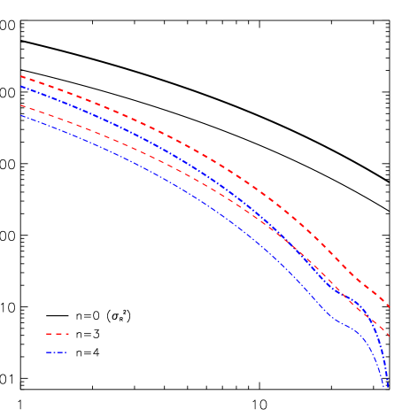
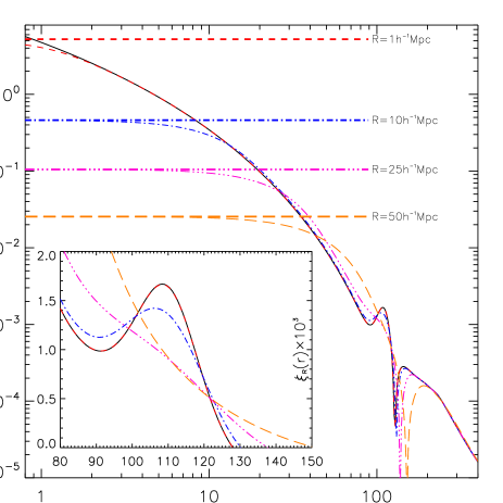
Figure 1: Left: the $2$-point correlation function of the smoothed mass density field $\xi_{R}$ is shown as a function of the smoothing scale $R$. We plot $\xi_{R}$ for different values of the correlation length $r=nR$ i.e. $n=0$ (black solid lines), $n=3$ (red dashed lines), and $n=4$ (blue dot-dashed lines) and at two different redshifts: $z=0$ (thick lines) and $z=1$ (thin lines). We adopt the linear power spectrum model of Eisenstein & Hu (1998) and we assume the following set of cosmological parameters: $\Omega_{m}=0.26$, $\Omega_{\Lambda}=0.74$, $H_{0}=72$ km s^-1 Mpc^-1, $\sigma_{8}(0)=0.79$, $\Omega_{b}=0.044$ and the spectral index $n_{s}=0.96$. Note that, for $n=0$, $\xi_{R}(0)=\sigma^{2}_{R}$, while for a correlation length that goes to infinity the correlation function of the smoothed density field tends to zero. The characteristic bump induced by the baryon acoustic oscillations becomes clearly visible as soon as $n$ is large enough. Right: the $2$-point correlation function $\xi_{R}(r)$ is shown as a function of the correlation length $r$ for fields smoothed on different scales, that is $R=1,10,25$ and $50h^{-1}$Mpc. As the smoothing scale $R$ tends to zero, one recovers the $2$-point correlation function of matter particles, while as the filtering scale becomes larger, the BAO peak is progressively suppressed. Note also that for $r\rightarrow 0$, the value of $\xi_{R}(r)$ saturates to the variance of the field on the given scale $R$. On the opposite sense ($r\rightarrow\infty$) all the curves converge to the value of the two-point correlation function of matter particles.

$\begin{array}[]{cc}\includegraphics[width=241.84842pt]{./fig2.ps}&\includegraphics[width=241.84842pt]{./fig3.ps}\end{array}$

Figure 2: Left : the logarithmic derivative of $\xi_{R}(r)$ with respect to $R$ (cfr. eq. 25) is shown as a function of the smoothing scale $R$ for different values of the correlation length $r=nR$ (i.e. for $n=0$ solid line, $n=3$ short-dashed line, $n=4$ dot-dashed line and $n=\infty$ long-dashed line). We have assumed the linear power spectrum model of Eisenstein & Hu (1998) and the same parameters value listed in the caption of Figure 1. The non-monotonic scaling of $\beta_{R}(nR)$ at a scale R$\sim 25h^{-1}$Mpc is induced by the baryon acoustic oscillations. Note that, in the linear regime, $\beta_{R}(r)$ does not depend on the cosmic epoch, i.e. it is a redshift independent quantity. Right : the scaling of the reduced correlator of order $3$ is shown as a function of the smoothing scale $R$ for different values of the correlation length $r=nR$. Note that for $n=0$ the correlator reduces to the skewness $S_{3,R}$ and that for $n=\infty$ the expression of $C_{12,R}(nR)$ reduces to the one adopted by Bernardeau (1996).

3 Galaxy Correlators

Smoothing is not the only process that leaves an imprint on the value of cumulant moments. Their amplitude and shape is also altered if galaxies, instead of massive particles, are used to trace the overall matter distribution. Fry & Gaztañaga (1993) computed the effects of biasing on one-point (smoothed) cumulant moments up to order $5$. In this section, we generalize those results by deriving the expressions of the smoothed two-point cumulant moments of the galaxy overdensity field up to the same order. These are new observables that can be used to test predictions of the GIP in the weakly non-linear regime, to give insight into the gravity induced large-scale bias, and also to distinguish models with Gaussian initial conditions from their non-Gaussian alternatives. Some of these possibilities will be explored in sections §4 and §5. Since from now on we only consider smoothed statistics, we simplify our notation by omitting any explicit reference to the smoothing scale $R$. The $R-$dependence of relevant statistical quantities will be re-emphasized when necessary.

Consider the $N$-point, smoothed, correlation functions of matter up to order $5$

$$\xi_{ij} = \kappa_{11}({\bf x}_{i},{\bf x}_{j})$$ (26)

$$\zeta_{ijk} = \kappa_{111}({\bf x}_{i},{\bf x}_{j},{\bf x}_{k})$$

$$\eta_{ijkl} = \kappa_{1111}({\bf x}_{i},{\bf x}_{j},{\bf x}_{k},{\bf x}_{l})$$

$$\omega_{ijklm} = \kappa_{11111}({\bf x}_{i},{\bf x}_{j},{\bf x}_{k},{\bf x}_{l},{\bf x}_{m}).$$

At leading order, the corresponding statistics describing the distribution of galaxies, labeled with the suffix ‘$g$’ are

$$\xi_{12,g} = {b_{1}}^{2}\,\xi_{12}$$ (27)

$$\zeta_{123,g} = {b_{{1}}}^{3}\,\zeta_{{123}}+{b_{{1}}}^{3}c_{{2}}\big{(}\xi_{{13}}\xi_{{23}}+2\ {\mathrm{p}erm}\big{)}$$

$$\eta_{1234,g} = {b_{{1}}}^{4}\,\eta_{{1234}}+{b_{1}}^{4}\big{[}c_{2}(\xi_{{23}}\zeta_{{124}}+11\ {\mathrm{p}erm})+c_{3}(\xi_{{14}}\xi_{{24}}\xi_{{34}}+3\ {\mathrm{p}erm})+{c_{2}}^{2}(\xi_{{13}}\xi_{{24}}\xi_{{34}}+11\ {\mathrm{p}erm})\big{]}$$

$$\omega_{12345,g} = {b_{{1}}}^{5}\,\omega_{{12345}}+{b_{1}}^{5}\big{[}c_{2}\left(\xi_{{15}}\eta_{{2345}}+19\ {\mathrm{p}erm}+\zeta_{{125}}\zeta_{{345}}+14\ {\mathrm{p}erm}\right)+c_{3}\left(\zeta_{{135}}\xi_{{25}}\xi_{{45}}+29\ {\mathrm{p}erm}\right)+$$

$$c_{4}\left(\xi_{{14}}\xi_{{24}}\xi_{{34}}\xi_{{45}}+4\ {\mathrm{p}erm}\right)+{c_{2}}^{2}\left(\zeta_{{135}}\xi_{{24}}\xi_{{25}}+119\ {\mathrm{p}erm}\right)+c_{2}c_{3}\left(\xi_{{14}}\xi_{{25}}\xi_{{34}}\xi_{{24}}+59\ {\mathrm{p}erm}\right)$$

$$+{c_{2}}^{3}\left(\xi_{{13}}\xi_{{24}}\xi_{{45}}\xi_{{15}}+59\ {\mathrm{p}erm}\right)\big{]}.$$

The mapping between correlators of mass ($\kappa_{nm}$) and galaxy ($\kappa_{nm,g}$) follows immediately by taking the two-point limiting case in the above expressions. Listed below are the results up to order $n+m=4$ (including also non-leading terms):

$$\kappa_{11,g} = b_{{1}}^{2}\kappa_{11}+b_{{1}}^{2}\big{(}c_{{3}}+C_{{12}}c_{{2}}\big{)}\kappa_{11}\,\kappa_{{2}}+1/2\,b_{{1}}^{2}c_{{2}}^{2}\kappa_{11}^{2}$$ (28)

$$\kappa_{12,g} = b_{{1}}^{3}(C_{{12}}+2\,c_{{2}})\kappa_{11}\,\kappa_{{2}}+b_{1}^{3}c_{2}\kappa_{11}^{2}+b_{{1}}^{3}\big{(}5/2\,c_{{3}}C_{{12}}+2\,c_{{2}}^{2}C_{{12}}+3\,c_{{3}}c_{{2}}+c_{{4}}+1/2\,c_{{2}}C_{{22}}+c_{{2}}^{2}S_{{3}}+c_{{3}}S_{{3}}$$

$$+c_{{2}}C_{{13}}\big{)}\kappa_{11}\,\kappa_{{2}}^{2}+b_{{1}}^{3}\big{(}c_{{2}}^{3}+1/2\,c_{{4}}+3\,c_{{2}}^{2}C_{{12}}+2\,c_{{3}}c_{{2}}+c_{{3}}C_{{12}}\big{)}\kappa_{11}^{2}\kappa_{{2}}+b_{{1}}^{3}c_{{3}}c_{{2}}\kappa_{11}^{3}$$

$$\kappa_{13,g} = {b_{{1}}}^{4}\big{(}6\,{c_{{2}}}^{2}+C_{{13}}+3\,c_{{2}}S_{{3}}+3\,c_{{3}}+6\,c_{{2}}C_{{12}}\big{)}\kappa_{11}\,{\kappa_{{2}}}^{2}+{b_{{1}}}^{4}\big{(}3\,C_{{12}}c_{{2}}+6\,{c_{{2}}}^{2}\big{)}{\kappa_{11}}^{2}\kappa_{{2}}+{b_{{1}}}^{4}c_{{3}}{\kappa_{11}}^{3}+{b_{{1}}}^{4}\big{(}3/2\,c_{{2}}C_{{14}}$$

$$+9/2\,C_{{12}}c_{{3}}S_{{3}}+12\,{c_{{2}}}^{2}c_{{3}}+6\,{c_{{2}}}^{3}S_{{3}}+45/2\,c_{{2}}c_{{3}}C_{{12}}+9\,c_{{2}}c_{{4}}+3/2\,c_{{3}}S_{{4}}+9/2\,c_{{4}}S_{{3}}+3/2\,c_{{5}}+15/2\,{c_{{3}}}^{2}+3\,{c_{{2}}}^{2}S_{{4}}$$

$$+3\,{c_{{2}}}^{2}C_{{22}}+15/2\,{c_{{2}}}^{2}C_{{12}}S_{{3}}+9/2\,c_{{4}}C_{{12}}+6\,{c_{{2}}}^{2}C_{{13}}+45/2\,c_{{3}}S_{{3}}c_{{2}}+5\,c_{{3}}C_{{13}}+6\,{c_{{2}}}^{3}C_{{12}}+1/2\,c_{{2}}C_{{23}}\big{)}\kappa_{11}\,{\kappa_{{2}}}^{3}$$

$$+{b_{{1}}}^{4}\big{(}9/2\,{c_{{2}}}^{2}{C_{{12}}}^{2}+6\,{c_{{2}}}^{2}C_{{13}}+3/2\,c_{{3}}C_{{22}}+39/2\,c_{{2}}c_{{3}}C_{{12}}+3/2\,c_{{4}}C_{{12}}+9/2\,c_{{3}}S_{{3}}c_{{2}}+3\,{c_{{2}}}^{4}+18\,{c_{{2}}}^{3}C_{{12}}$$

$$+3/2\,c_{{3}}{C_{{12}}}^{2}+15/2\,c_{{2}}c_{{4}}+18\,{c_{{2}}}^{2}c_{{3}}+6\,{c_{{2}}}^{3}S_{{3}}\big{)}{\kappa_{11}}^{2}{\kappa_{{2}}}^{2}+{b_{{1}}}^{4}\big{(}9/2\,{c_{{3}}}^{2}+1/2\,c_{{5}}+3/2\,c_{{4}}C_{{12}}+9\,c_{{2}}c_{{3}}C_{{12}}$$

$$+6\,{c_{{2}}}^{2}c_{{3}}\big{)}{\kappa_{11}}^{3}\kappa_{{2}}+3/2\,{b_{{1}}}^{4}c_{{2}}c_{{4}}{\kappa_{11}}^{4}$$

where $c_{i}\equiv b_{i}/b_{1}$ for $i\geq 2$. In appendix C, we list the expressions for the galaxy correlators up to order $5$. For ${\bf x}_{1}={\bf x}_{2}$, one recovers the expressions of Fry & Gaztañaga (1993) (cfr. their eq. 9). The leading term in eq. (28) reduces, in the one-point limiting case, to

$$\kappa_{2,g}=b_{1}^{2}\kappa_{2}.$$ (29)

We find that, to leading order in the product $\kappa_{11}\kappa_{2}$ the remaining results, $\kappa_{nm,g}$ for $n+m\geq 3$, preserve the hierarchical properties of matter correlators, i.e. $\kappa_{nm,g}=C_{nm,g}\kappa_{11,g}\kappa_{2,g}^{n+m-2}$, with amplitudes $C_{nm,g}$ given by

$$C_{12,g} = b_{1}^{-1}\big{(}C_{{12}}+2\,c_{{2}}\big{)}$$

$$C_{13,g} = b_{1}^{-2}\big{(}C_{{13}}+3\,c_{{2}}(S_{{3}}+2C_{{12}})+3\,c_{{3}}+6\,c_{{2}}^{2}\big{)}$$

$$C_{22,g} = b_{1}^{-2}\big{(}C_{{22}}+4\,c_{{2}}C_{{12}}+4\,{c_{{2}}}^{2}\big{)}$$ (30)

$$C_{14,g} = b_{1}^{-3}\big{(}C_{{14}}+4\,c_{{2}}(S_{{4}}+3\,C_{{13}})+12\,(c_{{3}}+3\,c_{{2}}^{2})(S_{{3}}+C_{{12}})+12\,c_{{2}}C_{{12}}S_{{3}}+4\,c_{{4}}+36\,c_{{3}}c_{{2}}+24\,c_{{2}}^{3}\big{)}$$

$$C_{23,g} = b_{1}^{-3}\big{(}C_{{23}}+2\,c_{{2}}(C_{{13}}+3\,C_{{22}})+3\,(c_{{3}}+c_{{2}}S_{{3}})C_{{12}}+6\,c_{{2}}^{2}(S_{{3}}+3\,C_{{12}})+6\,c_{{3}}c_{{2}}+12\,c_{{2}}^{3}\big{)}.$$

These relations show that in order to draw any conclusions from the galaxy distribution about matter correlations of order $N$, properties of biasing must be specified completely to order $N-1$. Note, also, that the equations (30) have been obtained in the large separation approximation and fail as soon as $|{\bf x}_{1}-{\bf x}_{2}|<R$. As a consequence, in the one-point limit they do not converge to the results of Fry & Gaztañaga (1993) on the amplitude of the reduce cumulants, that is

$$S_{{3,g}} = b_{1}^{-1}\left(S_{{3}}+3\,c_{{2}}\right)$$

$$S_{{4,g}} = b_{1}^{-2}\left(S_{{4}}+12\,c_{{2}}S_{{3}}+4\,c_{{3}}+12\,{c_{{2}}}^{2}\right)$$ (31)

$$S_{{5,g}} = b_{1}^{-3}\left(S_{{5}}+20\,c_{{2}}S_{{4}}+15\,c_{{2}}{S_{{3}}}^{2}+(30\,c_{{3}}+120\,{c_{{2}}}^{2})S_{{3}}+5\,c_{{4}}+60\,c_{{2}}c_{{3}}+60\,{c_{{2}}}^{3}\right).$$

Interestingly, the hierarchical scaling (cfr eq. (11)) is not the only matter property which survives to the local non-linear biasing transformation of eq. 1. We also find that

$$C_{22,g} = C_{12,g}C_{12,g}$$

$$C_{23,g} = C_{12,g}C_{13,g}$$ (32)

that is the reduced galaxy correlators $C_{nm,g}$, conserve the factorization property of the matter density field (cfr. eq. (12).)

4 Non linear bias in real space

The most common methods for estimating the amplitude of the non-linear bias coefficients $b_{i}$ rely upon fitting a theoretical model to higher order statistical observables, such as the 3-point correlation function (e.g. Gaztañaga & Scoccimarro, 2005), the bispectrum (e.g. Verde et al., 2002), or the galaxy probability distribution function (e.g. Marinoni et al., 2005).

In this section we take a different approach. We explicitly derive analytical relations directly expressing the non-linear bias coefficients $b_{i}$ as a function of high order observables. To this end we cannot simply invert the set of equations 30 (or 31), since the $N$th reduced galaxy correlator (or moment) are a function of $N+1$ bias coefficients. We add, instead, the expression of the 3rd order reduced correlator $C_{12,g}$ to the system of equations (31) and solve the resulting set for the biasing coefficients. We obtain

$$b_{1} = \frac{{\displaystyle 3\,C_{{12}}-2\,S_{{3}}}}{{\displaystyle 3\,C_{{12,g}}-2\,S_{{3,g}}}}$$ (33)

$$b_{2} = \frac{{\displaystyle(C_{{12}}S_{{3,g}}-S_{{3}}C_{{12,g}})(3\,C_{{12}}-2\,S_{{3}})}}{{\displaystyle(3\,C_{{12,g}}-2\,S_{{3,g}})^{2}}}$$ (34)

$$b_{3} = (9\,S_{{4,g}}C_{{12}}^{2}-12\,S_{{4,g}}C_{{12}}S_{{3}}+4\,S_{{4,g}}S_{{3}}^{2}-12\,S_{{3}}S_{{3,g}}C_{{12}}C_{{12,g}}+24\,S_{{3}}S_{{3,g}}^{2}C_{{12}}-24\,S_{{3}}^{2}S_{{3,g}}C_{{12,g}}+24\,S_{{3}}^{2}C_{{12,g}}^{2}$$

$$-9\,S_{{4}}C_{{12,g}}^{2}+12\,S_{{4}}C_{{12,g}}S_{{3,g}}-4\,S_{{4}}S_{{3,g}}^{2}-12\,S_{{3,g}}^{2}C_{{12}}^{2})(3\,C_{{12}}-2\,S_{{3}})\big{/}4(3\,C_{{12,g}}-2\,S_{{3,g}})^{3}$$

$$b_{4} = (-60\,{S_{{3}}}^{3}S_{{4,g}}C_{{12,g}}-108\,S_{{5,g}}{C_{{12}}}^{2}S_{{3}}-120\,S_{{4}}{S_{{3,g}}}^{3}S_{{3}}-600\,{S_{{3,g}}}^{3}S_{{3}}C_{{12}}^{2}+495\,S_{{4}}S_{{3}}C_{{12,g}}^{3}-600\,{S_{{3,g}}}^{2}S_{{3}}^{3}C_{12,g}$$

$$-270\,S_{{3,g}}S_{{4,g}}C_{{12}}^{3}+72\,S_{{5,g}}C_{{12}}S_{{3}}^{2}+108\,S_{{5}}C_{{12,g}}^{2}S_{{3,g}}+1200\,S_{{3,g}}S_{{3}}^{3}C_{{12,g}}^{2}+600\,S_{{3,g}}^{3}S_{{3}}^{2}C_{{12}}-40\,S_{{4}}S_{{3,g}}^{3}C_{{12}}$$

$$+120\,S_{{3,g}}S_{{4,g}}S_{{3}}^{3}-72\,S_{{5}}C_{{12,g}}S_{{3,g}}^{2}-90\,S_{{4}}S_{{3,g}}C_{{12}}C_{{12,g}}^{2}+120\,S_{{4}}S_{{3,g}}^{2}C_{{12}}C_{{12,g}}-930\,S_{{4}}S_{{3,g}}S_{{3}}C_{{12,g}}^{2}$$

$$+580\,S_{{4}}S_{{3,g}}^{2}S_{{3}}C_{{12,g}}+630\,S_{{3,g}}S_{{4,g}}C_{{12}}^{2}S_{{3}}-480\,S_{{3,g}}S_{{4,g}}C_{{12}}{S_{{3}}}^{2}+180\,S_{{3,g}}^{2}S_{{3}}C_{{12}}^{2}C_{{12,g}}-600\,S_{{3,g}}^{2}S_{{3}}^{2}C_{{12}}C_{{12,g}}$$

$$+270\,S_{{3,g}}S_{{3}}^{2}C_{{12}}C_{{12,g}}^{2}-135\,S_{{3}}S_{{4,g}}C_{{12}}^{2}C_{{12,g}}+180\,S_{{3}}^{2}S_{{4,g}}C_{{12}}C_{{12,g}}+54\,S_{{5,g}}C_{{12}}^{3}-16\,S_{{5,g}}S_{{3}}^{3}-54\,S_{{5}}C_{{12,g}}^{3}$$

$$+16\,S_{{5}}S_{{3,g}}^{3}+240\,S_{{3,g}}^{3}C_{{12}}^{3}-690\,S_{{3}}^{3}C_{{12,g}}^{3})(3\,C_{{12}}-2\,S_{{3}})\big{/}10(3\,C_{12,g}-2\,S_{3,g})^{4}.$$

This set of equations allow us to investigate the eventual non-linear character of the biasing function up to order $4$ by exploiting information encoded in the reduced correlators up to order $3$ and the reduced moments up to order $\leq 5$. In a forthcoming analysis we will investigate up to what precision the coefficients $b_{i}$ can be estimated using data of large redshift surveys such as BOSS, BigBOSS and EUCLID. Note that, if we set $\beta_{R}(r)=0$ in eq. (23), then our expressions for $b_{1}$ and $b_{2}$ (cfr. should eqs. (33) and (34)) reduce to equations (4) and (5) originally derived by Szapudi (1998). As stressed by this author, in this formalism biasing coefficients are not anymore simple parameters to be estimated (by maximizing, for example, the likelihood of observables that are sensitive to them such as the reduced skewness $S_{3}$ (Gaztañaga, 1994; Gaztañaga & Frieman, 1994), the bispectrum (Fry, 1994; Scoccimarro, 1998; Feldman et al., 2001; Verde et al., 2002), the 3-point correlation function (Gaztañaga & Scoccimarro, 2005; Pan & Szapudi, 2005) or the full probability distribution function of the density fluctuations Marinoni et al. (2005, 2008), but they become themselves estimators.

In what follows we will focus our analysis on the linear biasing parameter $b_{1}$ only. In our formalism, this quantity is explicitly expressed in terms of the amplitude of third-order statistics (i.e. the reduced cumulants and correlators) and it is independent from the amplitude of second-order statistics such as $\sigma_{R}$ and $\xi_{R}$. Notwithstanding, $b_{1}$ seems to depend on the shape of the power spectrum of the matter density fluctuations via the terms $\gamma_{R}$ and $\beta_{R}(r)$ that appears in eq. (23). We will demonstrate in the next session that the inclusion of the correction term $\beta_{R}(r)$ in our analysis has the additional advantage of making the linear bias coefficient $b_{1}$ effectively independent from any assumption about second order statistics, i.e. independent not only from the amplitude but also from the shape of the linear matter power spectrum. This fully third-order dependence of the linear biasing parameter estimator $b_{1}$ allows us to construct a consistent second-order estimator of the matter density fluctuations $\sigma_{R}$ on a given linear scale $R$.

5 The $rms$ fluctuations of the linear mass density field

Now that all the ingredients are collected, we detail how we construct our estimators of the linear matter density fluctuations $\sigma_{R}$. From eq. (22), (23), (29) and (33) we obtain

$$\sigma_{R}=\frac{\tau_{g,R}(r)}{\beta_{R}(r)-\gamma_{R}}\sigma_{g,R}$$ (37)

where

$$\tau_{g,R}(r)=3C_{12,g,R}(r)-2S_{3,g,R}$$ (38)

and where the suffix $g$ indicates that the relevant quantities are evaluated using data. For clarity, the scale dependence of third order statistics is explicitly highlighted. Apparently, the right-hand side of the above equations depends on the overall shape of the a-priori unknown matter power spectrum. In reality, the terms $\beta_{R}(r)-\gamma_{R}$ can be consistently estimated from observations without any additional theoretical assumption. To show this, we define

$$\alpha_{R}(r)\equiv\frac{d\log\eta_{R}(r)}{d\log R}$$ (39)

where

$$\eta_{R}(r)\equiv\frac{\xi_{R}(r)}{\sigma^{2}_{R}}.$$ (40)

As far as matter particles are considered, the previous definitions imply that $\alpha_{R}(r)=\beta_{R}(r)-\gamma_{R}$. By combining the expression for $\xi_{g,R}$ given by eq. 28 with its one-point limiting case i.e.

$$\sigma_{g,R}^{2}(z)=b_{1}^{2}\sigma_{R}^{2}(z)\left\{1+\left(1/2{c_{2}}^{2}+S_{3,R}c_{2}+c_{3}\right)\sigma_{R}^{2}(z)\right\},$$ (41)

and using the fact that, on scales where WNLPT applies, $\sigma_{R}^{2}\ll 1$, we obtain

$$\eta_{g,R}(r)\sim\eta_{R}(r)-\left\{(S_{3,R}-C_{12,R})c_{2}+1/2{c_{2}}^{2}\right\}\xi_{R}(r)+1/2{c_{2}}^{2}\eta_{R}(r)\xi_{R}(r),$$ (42)

where $\eta_{g,R}(r)=\xi_{g,R}(r)/\sigma^{2}_{g,R}$ and where the terms on the RHS have been sorted by order of magnitude. Finally, in the LS limit [$\xi_{R}(r)$ is negligible with respect to $\eta_{R}(r)$], the above equation reduces to $\eta_{g,R}(r)\sim\eta_{R}(r)$. The level of accuracy of this approximation is presented in Figure 3 where we show that, on a typical scale ($R\sim 16h^{-1}$ Mpc), the imprecision is less than $0.5\%$ at any cosmic epoch investigated ($0<z<0.6$). Since $\alpha_{g,R}(r)=\alpha_{R}(r)$, we obtain

$$\sigma_{R}=\frac{\tau_{g,R}(r)}{\alpha_{g,R}(r)}\sigma_{g,R}$$ (43)

where $\alpha_{g,R}(r)=d\log\eta_{g,R}(r)/d\log R$.

Counts-in-cells techniques provide and estimate of the terms on the RHS of eq. 43. In this regard, a central point worth stressing concerns the continuum-discrete connection. Biasing is not the only obstacle hampering the retrieval of matter properties from the analysis of galaxy catalogs. The formalism needs also to correct for the fact that the galaxy distribution is an intrinsically discrete process. These issues will be thoroughly addressed in Section §6.1 where we present the strategy that we have adopted in order to minimize the sampling noise.

Redshift space distortions are an additional effect that needs modeling. Results presented in the previous sections strictly hold in real (configuration) space. Therefore, the feasibility of extracting the value of mass fluctuations $\sigma_{R}$ via eq. (43) rests upon the possibility of expressing real space variables ($b_{1}^{-1}=\tau_{g,R}/\alpha_{g,R}$, and $\sigma_{g,R}$) in terms of redshift space observables. On the large (linear) cosmic scales where our formalism applies, the Kaiser model (e.g. Kaiser, 1987) effectively describes the mapping between real and redshift space expressions of second order statistics. The transformation is given by

$$\sigma_{g,R}^{z}=\left[1+\frac{2}{3}\frac{f}{b_{1}}+\frac{1}{5}\left(\frac{f}{b_{1}}\right)^{2}\right]^{1/2}\sigma_{g,R},$$ (44)

where the suffix $z$ labels measurements in redshift (as opposed to configuration) space, and where $f$ is the logarithmic derivative of the linear growth factor $D(a)$ with respect to the scale factor $a$. Much easier is the transformation rule for $\alpha_{g,R}$: in linear regime it is unaffected by redshift distortions, that is $\alpha^{z}_{g,R}=\alpha_{g,R}$.

Assessing the impact of peculiar motions on third order statistics is less straightforward. Up to now all the formulas were derived analytically from theory. To address this last issue we now use numerical simulations. By running some tests using a suite of simulated galaxy catalogs (described in section §6.2) we conclude that the amplitude of $S_{3,g}$ and $C_{12,g}$ are systematically (and non-negligibly) higher in $z$-space and that the relative overestimation systematically increases as a function of the order of the statistics considered (see Figures 5 and 6 in section §6.2). Notwithstanding, from the theoretical side, the expressions of third order statistics ($S_{3,R}=S_{3}+\gamma_{R}$ and $C_{12}=(2S_{3})/3+\gamma_{R}/3+\beta_{R}(r)/3$) imply that the linear combination $3C_{12,R}-2S_{3,R}$ should be much more insensitive to redshift distortions. Note, in particular, that both $\gamma_{R}$ and $\beta_{R}(r)$ are unaffected by linear motions. However convincing it might seem, this guess applies only to matter particles. In order to draw definitive conclusions about the impact of peculiar motions on $\tau_{g,R}$, we have used N-body galaxy simulations. Guided by synthetic catalogs we demonstrate that the biased galaxy statistics $\tau_{g,R}$ is effectively unaffected by redshift distortions. This conclusion is graphically presented in Figure 3 where we show that the relative error introduced by reconstructing the statistics using observed redshifts, instead of the cosmological ones, is progressively smaller as $R$ increases, and it is globally $<\sim 2\%$.

By incorporating these results into the formalism we finally obtain

$${\displaystyle\hat{\sigma}_{R}}=\sigma^{z}_{g,R}\Bigg{[}\bigg{(}\frac{\alpha^{z}_{g,R}}{\tau^{z}_{g,R}}\bigg{)}^{2}+\frac{2}{3}\frac{\alpha^{z}_{g,R}}{\tau^{z}_{g,R}}f+\frac{1}{5}f^{2}\Bigg{]}^{-1/2}$$ (45)

an estimator that is manifestly independent from any assumption about the amplitude and shape of the linear matter power spectrum. Also, this formula is independent from any assumption about the value of the Hubble constant $H_{0}$. Only an a-priori gravitational model must be assumed to correct for redshift space distortions in the local universe, that is to evaluate the growth rate function $f(z)$. This introduces an additional strong dependence on the cosmological parameters $\Omega_{M}$ and $\Omega_{\Lambda}$ on top of the marginal one that is forced upon when we compute metric distances in order to estimate $\sigma^{z}_{g,R}$, $\alpha^{z}_{g,R}(r)$ and $\tau^{z}_{g,R}$. More quantitatively, when the input cosmological parameters are chosen in the parameter plane delimited by $0\leq\Omega_{M}\leq 1$ and $0\leq\Omega_{\Lambda}\leq 1$ , the maximum relative variation of the estimates with respect to their fiducial value in the $\Lambda$CDM cosmological model are max$|df/f|\sim 0.6$, max$|d\tau/\tau|\sim 0.2$, max$|d\alpha/\alpha|=0.3$, and max$|d\sigma/\sigma|=0.15$. The weak cosmological dependence of $\tau^{z}_{g,R}$ follows from the fact that neither the reduced cumulants nor the reduced correlators of mass are effectively sensitive to the background cosmology. We expect them to be essentially unaffected also by sensible modifications of the gravitational theory (Gaztañaga & Lobo (2001), Multamaki et al. (2003), but see for example Freese & Lewis (2002) or Lue, Scoccimarro & Starkman (2001) for more radical scenarios where this expectation is not met). We have also noted that the denser in matter is the cosmological model the more overestimated are the values of both of $\alpha^{z}_{g,R}$ and $\tau^{z}_{g,R}$. Since also the amplitude of the cosmological dependence is nearly the same, we expect the ratio $\alpha^{z}_{g,R}/\tau^{z}_{g,R}$, i.e. the linear bias parameter, to be nearly insensitive to the underlying cosmological model. We have quantitatively verified this statement in Figure 11 of section §6.5. In conclusion, the estimator in eq. (45) is sensitive to cosmology mainly through the growth rate function $f(z)$ and, to some degree, through $\sigma^{z}_{g,R}$.

Once the cosmological background is known via independent techniques (e.g Astier et al. (2006); Komatsu et al. (2011); Marinoni & Buzzi (2010))) the strategy we have outlined offers the possibility to estimate in a direct way the amplitude and time evolution of matter fluctuations. The formalism could also be implemented, in a reverse direction, to probe the coherence of the gravitational instability paradigm. Any eventual discrepancy resulting from the comparison of the measurements (cfr. eq. (45)) with theoretical predictions (cfr. eq. (18)) provides evidence that either the assumed set of cosmological parameters are wrong, either the assumed power spectrum of matter fluctuations is poorly described by linear theory, either the time dependence of the linear growing mode $D(t)$ is deduced in the context of an improper gravitational model. This last testing modality will be explored in a further paper.

Figure 3: Left: the relative error arising from estimating the $\eta$-function using galaxies instead of matter. The inaccuracy ${\displaystyle\delta_{\eta}=\eta_{g,R}^{z}/\eta_{R}^{\;}-1}$ is evaluated at different epochs and is determined by assuming $R=16h^{-1}$Mpc and $r=3R$. Simulated data are extracted from the mock catalogs described in section §6.2. Right: relative difference between the real- and redshift-space estimation of $\tau_{g,R}\equiv 3C_{12,g}(r)-2S_{3,g}$. The inaccuracy $\delta_{\tau}=\tau_{g,R}^{z}(r)/\tau_{g,R}^{\;}(r)-1$ is plotted as a function of the smoothing scale $R$ and is computed at a separation $r=3R$. The dotted line represents the case in which computing the $\tau$ statistics using observed redshifts is equivalent to using cosmological redshifts. Real- and redshift-space simulated data are extracted from the mock catalogs described in section §6.2. In both panels the error bars represent $1\sigma$ standard deviation.

6 Applying the Method

The practical implementation of the method, including successful tests of its robustness, is discussed in this section. We first present a strategy to estimates the correlators of order $(n,m)$ of discrete 3D density fields such as those sampled by galaxy redshift surveys. We then show that, by applying the test formalism to N-body simulations of the large scale structure of the universe, we are able to recover the amplitude and scaling of the linear matter fluctuations $\sigma_{R}(z)$. A strategy to test the coherence of the results and to validate our conclusions is also designed, applied and discussed.

6.1 Statistical estimators of the galaxy correlators

The galaxy distribution is a discrete, 3-dimensional stochastic process. The random variable $N$ models the number of galaxies within typical cells (of constant comoving size) that ideally tesselate the universe or, less emphatically, a given redshift survey. Notwithstanding, a variable that is more directly linked to theoretical predictions of cosmological perturbation theory is the adimensional galaxy excess

$$\delta_{N}\equiv\frac{N}{\bar{N}}-1,$$ (46)

where $\bar{N}$ is the mean number of galaxies contained in the cells.

To estimate one-point moments of the galaxy overdensity field ($\mu_{n,g}=\langle\delta_{N}^{n}\rangle$), we fill the survey volume with the maximum number ($N_{t}$) of non-overlapping spheres of radius $R$ (whose center is called seed) and we compute

$$\hat{\mu}_{n,g}=\frac{1}{N_{t}}\sum_{i=1}^{N_{t}}\delta_{N,i}^{n},$$ (47)

where $\delta_{N,i}$ is the adimensional counts excess in the $i$-th sphere.

As far as two-point statistics are concerned, we add a motif around each previously positioned spheres. The center of each new sphere is separated from the seed by the length $r=nR$ and the pattern is designed in such a way to maximize the number of quasi non-overlapping spheres at the given distance $r$ (the maximum allowed overlapping between contiguous spheres is $2\%$ in volume.) The moments $\mu_{nm,g}=\langle\delta^{n}_{N,i}\delta^{m}_{N,j}\rangle$, that is the average of the excess counts over all the $i$ and $j$ spherical cells at separation $r$, are estimated as

$$\hat{\mu}_{nm,g}=\frac{1}{2N_{t}N_{mot}}\left\{\sum_{i=1}^{N_{t}}\delta_{N,i}^{n}\sum_{j=1}^{N_{mot}}\delta_{N,j}^{m}+\sum_{i=1}^{N_{t}}\delta_{N,i}^{m}\sum_{j=1}^{N_{mot}}\delta_{N,j}^{n}\right\},$$ (48)

where $N_{mot}$ is the number of spheres at distance $r$ from a given seed, and where we have assumed that the stochastic process is stationary. The expression of the one- and two-point cumulant moments $k_{nm,g}$ follows immediately from eq. (9).

Since galaxies counts are a discrete sampling of the underlying continuous stochastic field $\lambda_{g}({\bf x})$ (see section §2.1) it is necessary to correct our estimators for discreteness effects. In other terms, the quantity of effective physical interest that we want to estimate is $\delta_{g,R}({\bf x})\equiv\Lambda_{g}({\bf x})/{\bar{\Lambda}_{g}}-1$ where $\Lambda_{g}({\bf x})=\int_{V({\bf x})}\lambda({\bf x^{\prime}})d^{3}x^{\prime}$ is the continuous limit of the discrete counts N in the volume V. To this purpose, following standard practice in the field, we model the sampling as a local Poisson process (LPP, Layser (1956)) and we map moments of the discrete variable N into moments of its continuous limit by using

$$\langle\Lambda_{g}^{n}\rangle=\langle N(N-1)...(N-n+1)\rangle=\langle(N)_{f}^{n}\rangle,$$ (49)

in the case of one-point statistics, and its generalization (Szapudi & Szalay, 1997)

$$\langle\Lambda_{g}^{n}({\bf x}_{1})\Lambda_{g}^{m}({\bf x}_{2})\rangle=\langle(N_{1})_{f}^{n}(N_{2})_{f}^{m}\rangle,$$ (50)

for the two-point case. As a result, the estimators of $k_{nm,g}=\langle\delta^{n}_{g,R}(\vec{x})\delta^{m}_{g,R}(\vec{x}+\vec{r})\rangle_{c}$ corrected for shot noise effects are (Szapudi, Szalay & Boscàn, 1992; Angulo et al., 2008)

$$\hat{k}_{2,g} = \hat{\mu}_{2,g}-{\bar{N}}^{-1}$$ (51)

$$\hat{k}_{11,g} = \hat{\mu}_{11,g}$$

$$\hat{k}_{3,g} = \hat{\mu}_{3,g}-3{\bar{N}}^{-1}\hat{\mu}_{2,g}+2{\bar{N}}^{-2}$$

$$\hat{k}_{12,g} = \hat{\mu}_{12,g}-{\bar{N}}^{-1}\hat{\mu}_{11,g}$$

$$\hat{k}_{4,g} = \hat{\mu}_{4,g}-3\hat{\mu}_{2,g}^{2}-6{\bar{N}}^{-1}\hat{\mu}_{3,g}+11{\bar{N}}^{-2}\hat{\mu}_{2,g}-6{\bar{N}}^{-3}$$

$$\hat{k}_{13,g} = \hat{\mu}_{13,g}-3\hat{\mu}_{2,g}\hat{\mu}_{11,g}+2{\bar{N}}^{-2}\hat{\mu}_{11,g}-3{\bar{N}}^{-1}\hat{\mu}_{12,g}$$

$$\hat{k}_{22,g} = \hat{\mu}_{22,g}-2\hat{\mu}_{11,g}^{2}-\hat{\mu}_{2,g}^{2}+{\bar{N}}^{-2}\hat{\mu}_{11,g}-2{\bar{N}}^{-1}\hat{\mu}_{12,g}$$

$$\hat{k}_{5,g} = \hat{\mu}_{5,g}-10\hat{\mu}_{2,g}\hat{\mu}_{3,g}-10{\bar{N}}^{-1}\{\hat{\mu}_{4,g}-3{\hat{\mu}_{2,g}}^{2}\}+35{\bar{N}}^{-2}\hat{\mu}_{3,g}-50{\bar{N}}^{-3}\hat{\mu}_{2,g}+24{\bar{N}}^{-4}$$

$$\hat{k}_{14,g} = \hat{\mu}_{14,g}-6\hat{\mu}_{12,g}\hat{\mu}_{2,g}-4\hat{\mu}_{11,g}\hat{\mu}_{3,g}-6{\bar{N}}^{-1}\{\hat{\mu}_{13,g}-3\hat{\mu}_{11,g}\hat{\mu}_{2,g}\}+11{\bar{N}}^{-2}\hat{\mu}_{12,g}-6{\bar{N}}^{-3}\hat{\mu}_{11,g}$$

$$\hat{k}^{g}_{23,g} = \hat{\mu}_{23,g}-6\hat{\mu}_{11,g}\hat{\mu}_{12,g}-3\hat{\mu}_{2,g}\hat{\mu}_{12,g}-\hat{\mu}_{2,g}\hat{\mu}_{3,g}-3{\bar{N}}^{-1}\{\hat{\mu}_{22,g}-2{\hat{\mu}_{11,g}}^{2}-{\hat{\mu}_{2,g}}^{2}\}-{\bar{N}}^{-1}\{\hat{\mu}_{13,g}-3\hat{\mu}_{11,g}\hat{\mu}_{2,g}\}+5{\bar{N}}^{-2}\hat{\mu}_{12,g}+$$

$$-2{\bar{N}}^{-3}\hat{\mu}_{11,g}$$

where we have set $\hat{\mu}_{0i,g}=\hat{\mu}_{i0,g}\equiv\hat{\mu}_{i,g}$ and $\hat{k}_{0i,g}=\hat{k}_{i0,g}\equiv\hat{k}_{i,g}$.

$\begin{array}[]{cc}\includegraphics[width=227.62204pt]{./fig7.ps}&\includegraphics[width=227.62204pt]{./fig8.ps}\end{array}$

Figure 4: Left: the correlator of order $(1,1)$ of the smoothed galaxy overdensity field at the average redshift $z=0.34$ is shown as a function of the smoothing radius $R$, and for different values of the correlation length ($n=\{0,3,4\}$). In the degenerate case $n=0$ we recover the variance of the galaxy fluctuation field. Right: the redshift evolution of $\xi_{g,R}(nR)$ at a given smoothing scale ($R=17h^{-1}$Mpc) is shown for different values of the correlation length ($n=\{0,3,4\}$). The statistics are computed in both real (solid symbols) and redshift space (unfilled symbols). Each point is the average of the results obtained from 8 independent full-sky LRGs catalogs. Errorbars are estimated as the standard error of the mean.

$\begin{array}[]{cc}\includegraphics[width=227.62204pt]{./fig9.ps}&\includegraphics[width=227.62204pt]{./fig10.ps}\end{array}$

Figure 5: Left: the reduced correlator of order $(1,2)$ of the smoothed galaxy overdensity field at the average redshift $z=0.34$ is shown as a function of the smoothing radius $R$, and for different values of the correlation length ($n=0$ (upper panel) $n=3$ (central panel) and $n=4$ (lower panel)). In the degenerate case $n=0$ we recover the reduced skewness of the galaxy fluctuation field. Right: the redshift evolution of $C_{12,g,R}(nR)$ at a given smoothing scale ($R=17h^{-1}$Mpc) is shown for different values of the correlation length ($n=\{0,3,4\}$). The statistics are computed in both real (solid symbols) and redshift space (unfilled symbols). Each point is the average of the results obtained from 8 independent full-sky LRGs catalogs. Errorbars are estimated as the standard error of the mean.

Figure 6: Tthe reduced galaxy correlators of order 4 ($C_{13,g,R}$ and $C_{22,g,R}$) and of order 5 ($C_{23,g,R}$) at the average redshift $z=0.34$ and at the correlation separation $r=3R$ are shown as a function of the smoothing radius $R$. The statistics are computed in both real (solid symbols) and redshift space (unfilled symbols). Each point is the average of the results obtained from 8 independent LRGs catalogs. Errorbars are estimated as the standard error of the mean.

6.2 High order correlators extracted from cosmological simulations

We use numerical experiments simulating the spatial clustering of Luminous Red Galaxies (LRGs) of the Sloan Digital Sky Survey (SDSS) to validate the method, to test its end-to-end coherence and to spot the presence of eventual systematics. We have run the whole pipeline on two different simulations, namely Horizon (Kim et al., 2009; Dubinski et al., 2004; Kim & Park, 2006) and Las Damas (McBride et al., 2009). Ideally, this way, we are the least dependent upon the specific simulation strategy and technique. Since the outcome and salient features of the analysis are essentially the same, we here only present the analysis of the Horizon simulations. This is a large simulation ($4120^{3}$ particles in the box) in which LRGs galaxies are selected by finding the most massive gravitationally bound, cold dark matter halos. It is characterized by the following set of cosmological assumptions $(\Omega_{m}=0.26,\Omega_{\Lambda}=0.74,w_{0}=-1,w_{a}=0,H_{0}=72$km/s/Mpc,$\Omega_{b}=0.044,n_{s}=0.96,\sigma_{8}=0.79)$. We have analyzed 8 nearly independent, full-sky light cones extending over the interval $0.15<z<0.55$, each covering a volume of $13\;h^{-3}$Gpc³ and containing nearly $3.8\cdot 10^{6}$ LRGs galaxies. A mass threshold decreasing with redshift was chosen so to force Horizon’s comoving number density profile to be constant with redshift and reproduce the density profile observed in the SDSS LRGs sample. As a consequence, the simulated sample can be considered with good approximation as being volume limited. The mean comoving number density is $\bar{n}=3.0\times 10^{-4}\;h^{3}$Mpc^-3 and the mean inter-galaxy separation is $l\sim 19\;h^{-1}$Mpc. As an example, the average number of LRGs galaxies (${\bar{N}}$) inside a spherical cell of radius $R=(10,15,20,25)h^{-1}$Mpc is approximately $1,5,10$ and $20$.

In the left panel of Figure 4 we show the correlation function of the smoothed galaxy overdensity field $\xi_{g,R}=\langle\delta_{g,R}({\bf x})\delta_{g,R}({\bf x}+{\bf r})\rangle_{c}$ for different values of the correlation length ($r=nR$) in both real and redshift spaces. Note that in the degenerate case $n=0$ we recover the variance of the galaxy density fluctuations on a scale $R$. If the cell separation increases, the amplitude of the galaxy correlators of order 2 decreases. Their $R$-scaling is nearly similar to the slope of the analogous statistics computed for the matter density field (see Figure 2) with a slope of $\sim-2.25$ at $R=10h^{-1}$Mpc and $\sim-3.4$ at $R=20h^{-1}$Mpc for the correlation configuration $n=3$). Note also the neat appearance of the characteristic baryon acoustic peak at the scale $R\sim 25h^{-1}$Mpc when the correlation length is computed for $n=4$. We interpret these results as a qualitative indication of the fact that, at least on the scales explored by our analysis, the linear biasing parameter is well approximated in terms of a scale-free parameter.

On the right panel of Figure 4 we show the redshift dependence of the $\xi_{g,R}$ for a given arbitrary smoothing scale (in this case $R=17h^{-1}$Mpc). The constant amplitude of this statistic, together with the fact that the corresponding matter statistics decreases by no more than $\sim 0.05$ in amplitude over the same redshift interval ($0.15<z<0.55$, see Figure 8), provide evidences that linear biasing was nearly $\sim 15\%$ stronger at the early epoch $z=0.55$.

In Figure 5 we show the scaling of the one- and two-point reduced galaxy cumulant moments of order 3, namely $S_{3,g,R}$ and $C_{12,g,R}(r)$. The slight and systematic decrease of $S_{3,g,R}$ as a function of scales, much less pronounced than that of $S_{3,R}$ (see Figure 2), is not compatible with biasing being described by a single constant parameter $b_{1}$. Since, we have already argued that $b_{1}$ is scale independent, this implies that the biasing function is non linear and the next order biasing coefficient $b_{2}$ must show some scale dependency.

Additional information about the clustering of large scale structures can be retrieved from the analysis of the complementary third-order galaxy statistic, i.e. the reduced correlator $C_{12,g,R}(r=nR)$ on scales $R$ where this indicator is not too noisy. For both the correlation configurations $n=3$ and $n=4$ this requirement limits the region of interest to the scales $R\leq 25h^{-1}$Mpc. Despite the fact that measurements on different scales are correlated, it appears that both these statstics are fairly independent from $R$. We remark that in the LS limit the value of $C_{12,g,R}$ is also independent from the correlation scale $r$. As a consequence, eq. (43) is best evaluated by adopting the smallest possible value of $n$, i.e. the one that minimizes the amplitude of the errorbars.

Our analysis shows that both the amplitude of $S_{3,g,R}$ and $C_{12,g,R}(r)$ are nearly redshift independent, i.e. mostly independent from the cosmic epoch at which these statistics are computed. This property holds in both real and redshift spaces and mirrors the analogous behavior, predicted by theory, for the reduced cumulant moment of the matter field (see eqs. (22) and (23).) Because of this we can conclude that, at least up to redshift $z\sim 0.55$, even the next order biasing coefficient, i.e. $b_{2}$, is weakly sensitive to time in the Horizon simulations.

The WNLPT predicts that reduced moments and correlators of the matter field should display hierarchical properties in real space. Figure 5 shows that the scaling predicted by eq. (10) still holds in redshift space, a results originally found by Lahav et al. 1993 and Hivon et al. 1995 who showed that it holds even on smaller scales than those analyzed here, i.e. on domains where non-linear effects become important. In an analogous way, Figure (5) shows that the mapping between real and redshift space also preserves the hierarchical properties of the reduced correlator $C_{12,g}$. This property is not a characteristic of low orders statistics only. In Figure 6 we present the estimates of the galaxy reduced correlators up to order 5 in both real and redshift space. Observations in the local universe have shown that the reduced cumulants $S_{N,g,R}$ of the smoothed galaxy field in redshift space display hierarchical clustering properties up to order $N=6$ (e.g. Baugh et al. 2004). This plot shows that also the reduced correlators $C_{nm,g,R}$ extracted form the Horizon simulation preserve the hierarchical scaling up to order $5$ in redshift space. Note that, as already anticipated in section §5, the amplitude of the clustering is larger in redshift space and that the relative difference with respect to real space estimates increases systematically as a function of the order of the reduced correlators.

Finally, Figure 6 graphically displays the validity of the factorization property that we have found in eq. (LABEL:faco), i.e. that not all galaxy reduced correlators contain original information. We stress that even if the factorization property $C_{22,g}=C^{2}_{12,g}$ was shown to hold analytically only in real space, simulations now show that it holds also in redshift distorted space.

We conclude by commenting on the precision of the estimates. The relative error in the estimation of reduced correlators increases, as expected, with the order of the statistics. Moreover, two-point statistics are recovered with larger uncertainty than the one-point statistics of the same order since they are estimated using a smaller number of independent cells. Specifically we find that, the larger the correlation scale, the stronger the sensitivity of the estimates to finite volume effects. On the typical scale $R=20h^{-1}$Mpc the relative error with which $C_{12,g}$, $C_{13,g}$, $C_{14,g}$, $C_{22,g}$ and $C_{23,g}$ are recovered is $4$, $5$, $10$, $15$ and $33\%$ respectively. This can be compared to the precision with which the equal-order reduced moments $S_{N}$ have been estimated on the same scale, that is $0.7$, $2$ and $10\%$, for the order $3$, $4$ and $5$ respectively.

6.3 Estimation of $\sigma_{R}(z)$

In this section we test the efficiency of the estimator given in eq. (45). Three major potential issues, if not properly addressed, may affect its reliability. First, it is imperative to test whether we can safely apply WNLPT results in the LS approximation to compute the reduced correlators $C_{nm,R}(r)$ in the limit in which the cell separation is as low as $r\sim 3R$, as the analysis of Bernardeau (1996) suggests. Second, we want to verify that peculiar velocity corrections as well as redshift-space observations do not introduce unexpected biases into our real-space observables. Finally, we want to test if the local Poisson model fairly corrects for the sampling noise in the low counts regime.

To fulfill these goals, we apply the estimator given in eq. (45) to the simulated LRGs catalogs and gauge the precision with which we can retrieve the real-space amplitude and scaling of $\sigma_{R}$, that is both the local normalization and evolution of the linear matter perturbations embedded in the $\Lambda$CDM simulations.

The following argument help us to select the range of scales $R$ that are best suited for applying the formalism to the simulated catalogs. We expect that the estimator given in eq. (45) will work neatly on sufficiently large scales $R$ (where the WNLPT and the linear modeling of redshift distortions both apply) and on sufficiently large correlation lengths $r=nR$ (where the LS approximation applies). On the smallest scale where the method can be theoretically applied, i.e. $R=10h^{-1}$Mpc, the amplitude of $\sigma_{R}$, which is of order $\sim 0.4$ at the average redshift of the sample, is completely dominated by shot noise which is of the order $\sim 1$. The signal becomes dominant with respect to discrete sampling corrections as soon as $R$ is greater than $\sim 15h^{-1}$Mpc. Moreover, below this last scale, a small, but statistically significant imprecision arises in assuming $\tau_{g,R}=\tau^{z}_{g,R}$, as shown in Figure 3. On the opposite end, the largest scale $R$ accessible is set by the geometry of the survey and the requirement of sampling the correlation length $r=nR$ with sufficient statistical power. We find that the relative error in our estimate of $C_{12,g,R}(r)$ becomes larger than $\sim 10\%$ (see Figure 5) for scales $R>22h^{-1}$Mpc when $n=3$ and for scales $R>18h^{-1}$Mpc when $n=4$.

In Figure 7 we plot the estimates of $\sigma_{R}$ based on LRGs mock catalogs. We recover the $rms$ of the linear matter fluctuation field on two smoothing scales ($R=17$ and $20h^{-1}$Mpc) and for three different correlation lengths ($n=2$, $n=3$ and $n=4$). By contrasting our measurements against the theoretical predictions obtained by inserting into eq. (18) the parameters used in the Horizon simulations, we find that our reconstruction scheme fails when the correlation length is as low as $n=2$. This was expected since Bernardeau (1996) already showed that the LS approximation does not hold on such small correlation scales. Effectively, when we probe larger scales ($n=3$), the reconstruction becomes significantly more accurate (central panel of Figure 7), with the estimates of $\sigma_{R}$ at the average redshift of the catalog ($z=0.34$) being affected by a relative error of of $13\%$ and $15\%$ on the scales $R=17$ and $20h^{-1}$Mpc respectively. For $n=4$ errorbars become too large for the estimates to be also precise. Additionally, we remark that our estimates seem to slightly overestimate the value of $\sigma_{R}$ on both the scale analyzed. This is also confirmed by the analysis of an independent mock catalog, i.e. the Las Damas simulation (McBride et al., 2009). As stressed in section §2.3, this is due to the increasing inaccuracy in the theoretical prediction of the amplitude of the reduced correlators $C_{12,R}$ on correlation lengths that approaches the scale where $\xi_{R}$ crosses zero.

We re-emphasize that these estimates are totally independent from any assumption about shape and normalization of the power spectrum of linear matter fluctuations. They are also independent from the amplitude of the present day normalization of the Hubble parameter $H_{0}$. Our estimates, however, do depend on the set of cosmological parameters ($\Omega_{M},\Omega_{\Lambda}$) that we have used to assign galaxies to cells (i.e. to smooth the galaxy distribution), and to subtract the effect of redshift space distortions (i.e. to evaluate the growth rate function $f$).

6.4 Estimation of the local value of $\sigma_{8}$

As we have already discussed, the scale $R=8h^{-1}$Mpc falls outside the range of applicability of the test. Nonetheless, we can extract information about the value of $\sigma_{8}$ at redshift $z\sim 0$ ($\sigma_{8}(0)$) from measurements of $\sigma_{R}$ on larger scales. We do this by fitting eq. (18) to data. The price to pay is that the recovered value will depend on the adopted power spectrum model and on the set of parameters on which the power spectrum itself depends, i.e. the reduced Hubble constant $h$, the primordial spectral index $n_{s}$, and the reduced density of baryons ($\Omega_{b}$). This approach, however offer some advantage: if the relevant cosmological parameters $\Omega_{m}$, $\Omega_{\Lambda}$ and $h$ are considered known from independent probes, then we can extract information about the purely gravitational sector of the theory.

The way we proceed is as follows: we assume standard gravity as described by GR, we frame our analysis in the linear regime, i.e. we adopt the phenomenological description of the matter power spectrum given by Eisenstein & Hu (1998), as well as the time evolutionary model for $\sigma_{R}$ given in eq. (18), and we look for the the best fitting parameter $n_{s}$, $\Omega_{b}$ and $\sigma_{8}(0)$ that minimize the statistical distance between our measurements (cfr. eq. (45)) and theoretical predictions (cfr. eq. (18)). The outcome of this approach is displayed in Figure 8.

If we assume that $n_{s}$ and $\Omega_{b}$ are fixed to the simulation’s values $(n_{s}=0.96,\Omega_{b}=0.044)$, we obtain $\sigma_{8}(0)=0.79\pm 0.08$. This best fitting value is in perfect agreement with the simulated one ($\sigma_{8}=0.79$). Results obtained by performing a joint two-parameter analysis (after fixing the third parameter to the simulated value) are shown in Figure 9. The left and central panel of this figure reveal that $\sigma_{8}(0)$ is only marginally degenerate with respect to both $n_{s}$ and $\Omega_{b}$, a fact that highlights the fundamental inefficiency of our probe in constraining the values of both these parameters. This conclusion is reinforced in the right panel of the same figure, which displays a strong degeneracy between $n_{s}$ and $\Omega_{b}$ together with a loosely constrained confidence region in the corresponding parameters plane. Luckily, this means that the uncertainties with which both these parameters are estimated using more sensible probes, do not critically affect the precision with which our method constrain the amplitude of $\sigma_{8}(0)$.

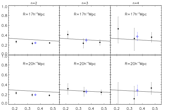
Figure 7: The real-space $rms$ of the matter fluctuation field is shown as a function of redshift. Black filled points represent estimates obtained by implementing eq. (45) to the LRGs mock catalogs. Solid lines show the theoretical prediction obtained by inserting all the physical and cosmological parameters of the Horizon simulation into eq. (18). Count-in-cell and cell correlation analyses have been performed by assuming spherical cells of radius $R$ separated by correlation lenght $r=nR$. We present results obtained for $n=2$ (left panels), $n=3$ (central panels) and $n=4$ (right panels) using two typical cell sizes $R=17h^{-1}$ Mpc (upper panels) and $R=20h^{-1}$Mpc (lower panels). Each point is the average of the results obtained from eight independent full-sky LRGs catalogs containing nearly 3.8 million galaxies each. Errorbars are estimated as the standard error of the mean. At the mean redshift of the catalogs ($z=0.34$) we also display the average estimate of $\sigma_{R}$ obtained in the whole survey volume (unfilled blue points).

Figure 8: The real-space $rms$ of the linear matter density fluctuations on a scale $R=17h^{-1}$Mpc is shown as a function of redshift. The same data as in the upper central panel of Figure 7 are used. The solid curve represents the best fitting theoretical model for the linear scaling of $\sigma_{17}$ (cfr. eq. (18) obtained after fixing the amplitude of $\Omega_{b}$, $n_{s}$ and $h$ to the values of the Horizon simulation. The corresponding best fitting value of $\sigma_{8}(0)$ is shown in the inset together with its standard deviation.

Despite the fact that our analysis was performed by slicing the survey volume in independent redshift shells, the limited redshift interval explored allows us to fix only the local amplitude of the linear matter fluctuation field. In a future work we will show that by implementing the method with deeper mock catalogs simulating the region of space that will be surveyed spectroscopically by surveys like BigBOSS and EUCLID, one can further aim at constraining the time evolution of $\sigma_{R}$. Data on a larger redshift interval will allow to constrain not only $\sigma_{8}(0)$, but also the growth index $\gamma$ in terms of which the growth rate is usually parameterized ($f=\Omega_{m}^{\gamma}(z)$ Peebles (1980)). This will allow to reject possible alternative description of gravity, or, in turn the standard model of gravitation itself.

6.5 Consistency tests

We have shown that, by using simulations, it is pretty straightforward to assess whether the proposed measuring strategy is able to recover the underlying value of $\sigma_{R}$. What if, instead, a real redshift survey is considered? Are there specific physical criteria or statistical indicators that guarantee us that the recovered value of $\sigma_{R}$ is the true one? In other terms we want to shift our attention from the precision of the estimates to their accuracy. Apart from the unbiasedness of the WNLPT results in the LS limit, our test strategy strongly relies on assuming that the correct set of cosmological parameters ($\Omega_{M}$, $\Omega_{\Lambda}$) has been used in the analysis. As a consequence, any imprecision in the measurements of the reduced cosmic densities translates into a biased estimate of $\sigma_{R}$. In this section, we design a diagnostic scheme to test the coherence of our results and, at the same time, the soundness of the adopted values for $\Omega_{M}$ and $\Omega_{\Lambda}$.

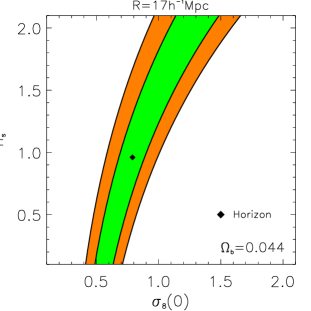
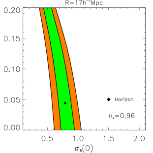
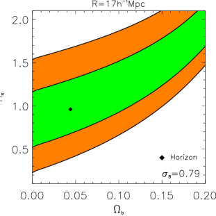
Figure 9: The likelihood contours obtained from the joint estimation of ($\sigma_{8}(0),n_{s}$), ($\sigma_{8}(0),\Omega_{b}$) and ($\Omega_{b},n_{s}$). The analysis have been performed calculating reduced correlators on a scale $R=17h^{-1}$Mpc and at the correlation lenght $n=3$. Isocontours of differently colored region corresponds to $\mathcal{L}_{min}+2.30$ and $\mathcal{L}_{min}+4.61$ where $\mathcal{L}$ is proportional to the log of the likelihood of the data and it is here assumed to be affine to the $\chi^{2}$ statistic.. On each panel the filled points represent the fiducial value of the Horizon simulation.

In the approach developed in this paper, the linear biasing parameter in real space is directly estimated from redshift space observables of intrinsic third-order nature using the estimator

$$b_{1,R}=\frac{\alpha^{z}_{g,R}}{\tau^{z}_{g,R}}.$$ (52)

As discussed in Section §5, this estimator has the remarkable property of being approximately independent from cosmology.

Now let’s define two new estimators of the real space linear biasing parameter as $\mathring{b}_{1,R}=\sigma_{g,R}/\sigma_{R}$ and $\tilde{b}_{1,R}=\sqrt{\xi_{g,R}/\xi_{R}}$, where now we exploit, as it is usual, second order statistics. Both $\sigma_{g,R}$ and $\xi_{g,R}$ are quantities not directly measurable, nonetheless we can recast the expressions of the real space linear biasing parameters in terms of redshift space observables. By adopting the Kaiser model for linear motions we obtain

$$\displaystyle\mathring{b}_{1,R} = -\frac{f}{3}+\sqrt{\left(\frac{\sigma_{g,R}^{z}}{\sigma_{R}}\right)^{2}-\frac{4}{45}f^{2}}$$ (53)

$$\displaystyle\tilde{b}_{1,R} = -\frac{f}{3}+\sqrt{\frac{\xi_{g,R}^{z}}{\xi_{R}}-\frac{4}{45}f^{2}}.$$ (54)

Before proceeding further, note that in this paper we have assumed that the Kaiser linear modeling of redshift space distortions applies on the scales we are interested in. We can now verify this statement by using the LRGs synthetic catalogs. To this purpose, and without loss of generality, be $\tilde{b}_{1,R}$ the value of the real-space linear bias parameter estimated from the mock catalogs as $\sqrt{\xi_{g,R}/\xi_{R}}$. Let’s refer to this estimate as to the true value of the linear-bias parameter and let’s label it as $b_{1}^{th}$. In figure 10 we compare these measurements against the estimates of the real-space linear bias inferred using eq. (54) in three different redshift intervals and for various smoothing scales $R$. One can see that for $n=3$, the estimator (54) fairly recovers the real-space value of the linear bias parameter. This result lends support to the hypothesis that, at least in the Horizon simulations, and over the range of $R$ scales where we trust the correlator’s theory, the distortions induced by large scale peculiar motions are accurately described by the Kaiser model.

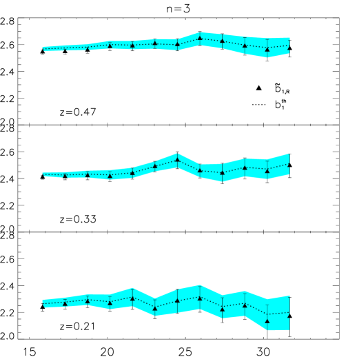
Figure 10: Black triangles show the $R$ dependence of the real-space linear bias parameter $\tilde{b}_{1,R}$ estimated from redshift-space mock catalogs using eq. (54). Measurements are performed using the correlation length $n=3$ and in three different redshift bins. These measurements are compared to the real-s[ace linear bias parameter $b_{1}^{th}$ extracted from real-space mock catalogs using the estimator $\sqrt{\xi_{g,R}/\xi_{R}}$ (dotted line). The shaded area represents the region of $1$-$\sigma$ uncertainty.

Physically, we expect that, whatever is the chosen scale $R$, if $\sigma_{8}(0)$ has been consistently determined, then eqs. (52), (53) and (54) all give the same numerical result. Since the linear biasing estimators given in eqs. (53) and (54) depends on the chosen background cosmology, the correct set of cosmological parameters is thus the very one that makes all the three different linear biasing definitions converge to the same numerical value on all the scale $R$. In a different paper (Bel & Marinoni in prep) we show how this observation can be exploited to guess the background cosmology. In this paper, we use this property to gauge the consistency of our measurements of $\sigma_{R}$, that is to verify that all the different estimators of the linear biasing parameters match only when the analysis is carried out in the proper cosmological background.

In Figure 11 we perform this test and show what pathological features do show up when the analysis relies on an improperly chose set of values ($\Omega_{M},\Omega_{\Lambda}$). The algorithm goes as follows: we estimate $\sigma_{R}$ on a given arbitrary scale $R$ (here we chose $R=16h^{-1}$Mpc), and in four different cosmologies (indicated in each panel of Figure 11). We then deduce the value of $\sigma_{8}(0)$ in each of these four scenarios. In doing this, we implicitly assume that the specific cosmology adopted in order to measure $\sigma_{R=16}$ is the correct one and that, as a consequence, the value of $\sigma_{8}(0)$ inferred using any other scale $R$ is identically the same. We then plug in this value of $\sigma_{8}(0)$ into eqs. eqs. (53) and (54) and compare the results with those obtained via the estimator $b_{1,R}$, i.e. we contrast them against a measurement of the linear biasing parameter that is weakly sensitive to cosmology.

If we analyze the LRGs mock catalogs by assuming the simulated set of cosmological parameters ($\Omega_{M}=0.26,\Omega_{\Lambda}=0.74$, see upper left panel of Figure 11) then the estimates of $\mathring{b}_{1,R}$, $\tilde{b}_{1,R}$ and $b_{1,R}$ are consistent between themselves on all the scales $R$. On the contrary, if we process data by incorrectly assuming a low density (open) background model (upper right panel in Figure 11), the different estimations of the linear biasing parameter are not anymore in agreement, even if the estimated value of $\sigma_{8}(0)$ has not changed (note that the linear power spectrum at present epoch is independent from the amplitude of the cosmological constant and thus insensitive to its variation). In particular, $\mathring{b}_{1,R}$ identically coincides, by definition, with the measure obtained using our estimator $b_{1,R}$ only for $R=16h^{-1}$Mpc , but the estimates deviate on all the other scales. This discrepancy is due to the fact that, in a “wrong” cosmology, the extrapolated value of $\sigma_{8}(0)$ may not be independent from the scale $R$ on which $\sigma_{R}$ is measured. Or said differently, the equation $\mathring{b}_{1,R}(\sigma_{8}(0))=b_{1,R}$ might not have a unique solution $\sigma_{8}(0)$ for all the scales $R$.

The effect previously discussed is mostly the consequence of adopting the wrong amplitude for the cosmological constant. It is, however, less pronounced than the discrepancy between the measurements of $\mathring{b}_{1,R}$ and $\tilde{b}_{1,R}$ that arises when the value of $\Omega_{m}$ is poorly guessed. The effects of a wrong choice of the matter density parameter are presented in the lower panels of Figure 11. The observed large inconsistency arises essentially from the fact that the zero order spherical Bessel function appearing inside the integral in eq. (21) filters in different portions of the signal (i.e. of $\Delta^{2}_{L}$) if the characteristic parameters of the linear power spectrum are changed. In other terms, if we consider eq. (21) and spuriously overestimate $\Omega_{m}$, the predicted suppression of power on a scales $r$ is larger than the variation actually seen in the data.

We remark that our estimator of the linear biasing parameter, relying on third-order statistical indicators, is affected by errorbars that are larger than those associated to the classical estimators $\mathring{b}_{1,R}$ and $\tilde{b}_{1,R}$. This imprecision is largely compensated by the fact that our estimator does not depend on any assumption about the nature of the dark matter (i.e. the specific form of the matter power spectrum) and it is almost insensitive also to its abundance ($\Omega_{M}$). Therefore, by contrasting different estimations of the linear biasing parameter, using the diagnostic diagram of Figure 11, we can deduce if the scaling of $\sigma_{R}$ was inferred in the appropriate cosmological model.

Figure 11: Comparison between the values of the linear bias parameter on various scales $R$. Measurements are obtained using $3$ different estimators (cfr. eqs. (52), (53), and (54)) and by analyzing the same redshift data in 4 different cosmological backgrounds as specified in the panels. $\mathring{b}_{1,R}$ and $\tilde{b}_{1,R}$ are estimated on the basis of the best fitting value of $\sigma_{8}(0)$ indicated in each panel. This last value has been obtained from measurements of $\sigma_{R}$ on a scale $R=16h^{-1}$Mpc and by assuming, arbitrarily, that the linear power spectrum parameters are subject to the following constraints: $h=0.72$ and $\Omega_{b}/\Omega_{m}=0.17$ for all the cosmological models. Note that in the lower panel, $\tilde{b}_{1,R}$ data are missing on a scales $R=(19,20)h^{-1}$Mpc. This is due to the fact that the argument of $\sqrt{\xi_{g,R}/\xi_{R}}$ is negative, i.e. in these extreme cosmological models, the predicted correlation function of the matter density field becomes negative on scales where the corresponding galaxy statistic is still positive. The horizontal dotted line shows the average of the measurements obtained with our estimators $b_{1,R}$ in the true cosmological model (i.e. the $\Lambda$CDM model of the Horizon simulation) and it is reproduced identically in all the panels. This line graphically helps to highlight the relative insensitivity of our estimator $b_{1,R}$ to the choice of the parameters ($\Omega_{M},\Omega_{\Lambda}$). Note how different estimates converge to the same value only when the analysis is performed in the true cosmological model.

Conclusions

A key goal that seems to fall within the technical reach of future cosmological experiments is to rule out (or in) eventual infrared modifications of the standard theory of gravity, as possibly manifested by the unexpected growth of cosmic mass in the weakly non-linear, low-curvature, high-redshift regimes. To fulfill this task, it is mandatory to devise sensible observables of the large scale structure of the universe. In this spirit, this paper focuses on the potential of clustering indicators that have been rarely explored in literature, that is the high-order reduced correlators $C_{nm}$ of the 3D mass overdensity field.

To fully exploit the richness of information contained in this two-point statistics, whose amplitude is analytically predicted by the weakly non-linear perturbation theory in the large separation limit approximation, we have derived the expressions of the reduced correlators of the smoothed galaxy density field ($C_{nm,g}$) up to order $5$. We have found that they preserve both the hierarchical scaling and the factorization properties of the matter reduced correlators.

Building upon these results we have worked out the explicit expressions for the bias coefficients up to order $4$ and a new estimator to measure the $rms$ of the linear matter fluctuations on a scale $R$ directly from galaxy redshift surveys. The central result of this paper, namely the estimator given in eq. (45), has been tested using artificial galaxy catalogs and shown to recover fairly well the ‘hidden’ simulated value of $\sigma_{R}$.

Despite the fact that very large survey volume are needed to make the estimation of these observables accurate enough for cosmological purposes, the merit of this approach are evident: a) linear biasing is not a parameter that one needs to marginalize over, but a physical parameter that can be estimated in a totally independently way from any assumption about the structure of the linear power spectrum and the value of cosmological parameters. b) the real space linear biasing parameter can be measured directly using redshift space observables. c) The scaling of $\sigma_{R}$ can be inferred directly without imposing any a-priori constraint on the eventual non-linear and scale dependent nature of the bias function. d) The correlator formalism allows also for a self-consistent test of the coherence of the results obtained concerning the scaling of $\sigma_{R}$, a step further in the direction of making cosmological results not only precise but also accurate.

In this paper we have analyzed local simulations with the aim of testing principles and theoretical ingredients on which the proposed strategy relies. Work is already in progress to apply the formalism to the SDSS-dr7 data and to extract the local value of linear matter fluctuations on sensible scales $R$. The good news is that the next decade holds even greater prospects for growth of the red-shifts data base. Therefore, we also plan to implement the algorithm to mock catalogs simulating future large 3D surveys such as BigBOSS and EUCLID and forecast up to what order and precision the bias coefficients $b_{i}$ can be estimated, as well as, the figure of merit achievable on $\sigma_{8}$ and on the gravitational growth index $\gamma$.

From the theoretical side, valuable insights are expected from a reverse engineering on the proposed test. For example, we show in a different paper (Bel & Marinoni in prep.) that if the gravitational model is a-priori known then the formalism offers the possibility of narrowing in on the value of fundamental cosmological parameters such as $\Omega_{m}$ and $\Omega_{\Lambda}$. Also further work is needed to understand how higher order real-space biasing parameters can be effectively retrieved from redshift space reduced correlators. Finally, interesting possibilities will open up if WNLPT predictions could be extended into the small separation limit where much more statistical power is locked.

CM is grateful for support from specific project funding of the Institut Universitaire de France. We thank the anonymous referee for his comments and suggestions. We acknowledge useful discussions with E. Branchini, E. Gaztañaga, L. Guzzo, L. Moscardini.

Appendix A Appendix A: higher order galaxy two-point cumulant moments

Listed here are the amplitudes of the two-point galaxy cumulant moments. Correlators of the galaxy distribution have been computed up to order 5.

$$\kappa_{g,11} = {b_{{1}}}^{2}\kappa_{11}+{b_{{1}}}^{2}\big{(}c_{{3}}+C_{{12}}c_{{2}}\big{)}\kappa_{11}\,\kappa_{{2}}+1/2\,{b_{{1}}}^{2}{c_{{2}}}^{2}{\kappa_{11}}^{2}$$

$$\kappa_{g,12} = {b_{{1}}}^{3}\big{(}C_{{12}}+2\,c_{{2}}\big{)}\kappa_{11}\,\kappa_{{2}}+{b_{{1}}}^{3}\big{(}5/2\,c_{{3}}C_{{12}}+2\,{c_{{2}}}^{2}C_{{12}}+3\,c_{{3}}c_{{2}}+c_{{4}}+1/2\,c_{{2}}C_{{22}}+{c_{{2}}}^{2}S_{{3}}+c_{{3}}S_{{3}}+c_{{2}}C_{{13}}\big{)}\kappa_{11}\,{\kappa_{{2}}}^{2}$$

$$+{b_{{1}}}^{3}\big{(}{c_{{2}}}^{3}+1/2\,c_{{4}}+3\,{c_{{2}}}^{2}C_{{12}}+2\,c_{{3}}c_{{2}}+c_{{3}}C_{{12}}\big{)}{\kappa_{11}}^{2}\kappa_{{2}}+{b_{{1}}}^{3}c_{{3}}c_{{2}}{\kappa_{11}}^{3}$$

$$\kappa_{g,13} = {b_{{1}}}^{4}\big{(}6\,{c_{{2}}}^{2}+C_{{13}}+3\,c_{{2}}S_{{3}}+3\,c_{{3}}+6\,c_{{2}}C_{{12}}\big{)}\kappa_{11}\,{\kappa_{{2}}}^{2}+{b_{{1}}}^{4}\big{(}3\,C_{{12}}c_{{2}}+6\,{c_{{2}}}^{2}\big{)}{\kappa_{11}}^{2}\kappa_{{2}}+{b_{{1}}}^{4}c_{{3}}{\kappa_{11}}^{3}+{b_{{1}}}^{4}\big{(}3/2\,c_{{2}}C_{{14}}$$

$$+9/2\,C_{{12}}c_{{3}}S_{{3}}+12\,{c_{{2}}}^{2}c_{{3}}+6\,{c_{{2}}}^{3}S_{{3}}+{\frac{45}{2}}\,c_{{2}}c_{{3}}C_{{12}}+9\,c_{{2}}c_{{4}}+3/2\,c_{{3}}S_{{4}}+9/2\,c_{{4}}S_{{3}}+3/2\,c_{{5}}+15/2\,{c_{{3}}}^{2}+3\,{c_{{2}}}^{2}S_{{4}}$$

$$+3\,{c_{{2}}}^{2}C_{{22}}+15/2\,{c_{{2}}}^{2}C_{{12}}S_{{3}}+9/2\,c_{{4}}C_{{12}}+6\,{c_{{2}}}^{2}C_{{13}}+{\frac{45}{2}}\,c_{{3}}S_{{3}}c_{{2}}+5\,c_{{3}}C_{{13}}+6\,{c_{{2}}}^{3}C_{{12}}+1/2\,c_{{2}}C_{{23}}\big{)}\kappa_{11}\,{\kappa_{{2}}}^{3}$$

$$+{b_{{1}}}^{4}\big{(}9/2\,{c_{{2}}}^{2}{C_{{12}}}^{2}+6\,{c_{{2}}}^{2}C_{{13}}+3/2\,c_{{3}}C_{{22}}+{\frac{39}{2}}\,c_{{2}}c_{{3}}C_{{12}}+3/2\,c_{{4}}C_{{12}}+9/2\,c_{{3}}S_{{3}}c_{{2}}+3\,{c_{{2}}}^{4}+18\,{c_{{2}}}^{3}C_{{12}}+3/2\,c_{{3}}{C_{{12}}}^{2}$$

$$+15/2\,c_{{2}}c_{{4}}+18\,{c_{{2}}}^{2}c_{{3}}+6\,{c_{{2}}}^{3}S_{{3}}\big{)}{\kappa_{11}}^{2}{\kappa_{{2}}}^{2}+{b_{{1}}}^{4}\big{(}9/2\,{c_{{3}}}^{2}+1/2\,c_{{5}}+3/2\,c_{{4}}C_{{12}}+9\,c_{{2}}c_{{3}}C_{{12}}+6\,{c_{{2}}}^{2}c_{{3}}\big{)}{\kappa_{11}}^{3}\kappa_{{2}}$$

$$+3/2\,{b_{{1}}}^{4}c_{{2}}c_{{4}}{\kappa_{11}}^{4}$$

$$\kappa_{g,22} = {b_{{1}}}^{4}\big{(}4\,c_{{2}}C_{{12}}+4\,{c_{{2}}}^{2}+C_{{22}}\big{)}\kappa_{11}\,{\kappa_{{2}}}^{2}+{b_{{1}}}^{4}\big{(}4\,c_{{3}}+8\,C_{{12}}c_{{2}}+4\,{c_{{2}}}^{2}\big{)}{\kappa_{11}}^{2}\kappa_{{2}}+4\,{b_{{1}}}^{4}{c_{{2}}}^{2}{\kappa_{11}}^{3}+{b_{{1}}}^{4}\big{(}2\,{c_{{2}}}^{2}C_{{22}}$$

$$+2\,{c_{{2}}}^{2}C_{{12}}S_{{3}}+4\,c_{{3}}C_{{22}}+4\,{c_{{2}}}^{3}S_{{3}}+2\,c_{{2}}C_{{23}}+12\,c_{{2}}c_{{3}}C_{{12}}+2\,C_{{12}}c_{{3}}S_{{3}}+8\,{c_{{2}}}^{2}c_{{3}}+4\,{c_{{2}}}^{2}C_{{13}}+4\,c_{{2}}c_{{4}}+4\,c_{{3}}S_{{3}}c_{{2}}$$

$$+4\,{c_{{2}}}^{3}C_{{12}}+2\,c_{{4}}C_{{12}}\big{)}\kappa_{11}\,{\kappa_{{2}}}^{3}+{b_{{1}}}^{4}\big{(}2\,{c_{{2}}}^{4}+6\,c_{{3}}S_{{3}}c_{{2}}+8\,{c_{{2}}}^{2}C_{{22}}+2\,c_{{4}}S_{{3}}+4\,c_{{3}}{C_{{12}}}^{2}+10\,{c_{{2}}}^{2}{C_{{12}}}^{2}+8\,c_{{4}}C_{{12}}+10\,{c_{{3}}}^{2}$$

$$+2\,c_{{5}}+36\,c_{{2}}c_{{3}}C_{{12}}+8\,{c_{{2}}}^{2}c_{{3}}+4\,{c_{{2}}}^{2}C_{{13}}+12\,{c_{{2}}}^{3}C_{{12}}+4\,c_{{3}}C_{{13}}+6\,c_{{2}}c_{{4}}\big{)}{\kappa_{11}}^{2}{\kappa_{{2}}}^{2}+{b_{{1}}}^{4}\big{(}8\,c_{{2}}c_{{4}}+16\,{c_{{2}}}^{3}C_{{12}}$$

$$+20\,c_{{2}}c_{{3}}C_{{12}}+16\,{c_{{2}}}^{2}c_{{3}}\big{)}{\kappa_{11}}^{3}\kappa_{{2}}+{b_{{1}}}^{4}\big{(}2{c_{{3}}}^{2}+{c_{{2}}}^{4}+4\,{c_{{2}}}^{2}c_{{3}}\big{)}{\kappa_{11}}^{4}$$

$$\kappa_{g,14} = {b_{{1}}}^{5}\big{(}C_{{14}}+24\,{c_{{2}}}^{3}+12\,c_{{3}}S_{{3}}+4\,c_{{4}}+12\,c_{{2}}C_{{12}}S_{{3}}+36\,{c_{{2}}}^{2}S_{{3}}+12\,c_{{2}}C_{{13}}+36\,{c_{{2}}}^{2}C_{{12}}+4\,c_{{2}}S_{{4}}+12\,c_{{3}}C_{{12}}$$

$$+36\,c_{{3}}c_{{2}}\big{)}\kappa_{11}\,{\kappa_{{2}}}^{3}+{b_{{1}}}^{5}\big{(}36\,{c_{{2}}}^{2}C_{{12}}+4\,c_{{2}}C_{{13}}+3\,c_{{2}}{C_{{12}}}^{2}+36\,{c_{{2}}}^{3}+12\,c_{{3}}c_{{2}}+12\,{c_{{2}}}^{2}S_{{3}}\big{)}{\kappa_{11}}^{2}{\kappa_{{2}}}^{2}+{b_{{1}}}^{5}\big{(}6\,c_{{3}}C_{{12}}$$

$$+12\,c_{{3}}c_{{2}}\big{)}{\kappa_{11}}^{3}\kappa_{{2}}+{b_{{1}}}^{5}c_{{4}}{\kappa_{11}}^{4}+{b_{{1}}}^{5}\big{(}42\,c_{{2}}c_{{3}}{S_{{3}}}^{2}+12\,c_{{3}}S_{{3}}C_{{13}}+8\,c_{{3}}C_{{12}}S_{{4}}+2\,c_{{6}}+90\,{c_{{2}}}^{3}C_{{12}}S_{{3}}+24\,{c_{{2}}}^{2}C_{{13}}S_{{3}}$$

$$+20\,{c_{{2}}}^{2}C_{{12}}S_{{4}}+6\,{c_{{2}}}^{2}C_{{22}}S_{{3}}+180\,c_{{3}}{c_{{2}}}^{2}C_{{12}}+84\,c_{{2}}c_{{3}}C_{{13}}+282\,{c_{{2}}}^{2}c_{{3}}S_{{3}}+6\,c_{{2}}c_{{3}}C_{{22}}+62\,c_{{2}}c_{{3}}S_{{4}}+74\,c_{{2}}c_{{4}}C_{{12}}$$

$$+114\,c_{{2}}c_{{4}}S_{{3}}+24\,c_{{4}}S_{{3}}C_{{12}}+168\,c_{{2}}c_{{3}}S_{{3}}C_{{12}}+8\,c_{{5}}C_{{12}}+24\,c_{{2}}c_{{5}}+12\,c_{{5}}S_{{3}}+12\,c_{{4}}C_{{13}}+8\,c_{{4}}S_{{4}}+6\,c_{{4}}{S_{{3}}}^{2}$$

$$+72\,c_{{4}}{c_{{2}}}^{2}+44\,c_{{3}}c_{{4}}+54\,{c_{{3}}}^{2}C_{{12}}+84\,{c_{{3}}}^{2}S_{{3}}+114\,{c_{{3}}}^{2}c_{{2}}+60\,{c_{{2}}}^{3}c_{{3}}+17/2\,c_{{3}}C_{{14}}+2\,c_{{3}}S_{{5}}+1/2\,c_{{2}}C_{{2,4}}+2\,c_{{2}}C_{{1,5}}$$

$$+6\,{c_{{2}}}^{2}S_{{5}}+18\,{c_{{2}}}^{3}C_{{22}}+24\,{c_{{2}}}^{3}{S_{{3}}}^{2}+6\,{c_{{2}}}^{2}C_{{23}}+36\,{c_{{2}}}^{3}C_{{13}}+36\,{c_{{2}}}^{4}S_{{3}}+18\,{c_{{2}}}^{2}C_{{14}}+24\,{c_{{2}}}^{4}C_{{12}}+36\,{c_{{2}}}^{3}S_{{4}}\big{)}\kappa_{11}\,{\kappa_{{2}}}^{4}$$

$$+{b_{{1}}}^{5}\big{(}2\,c_{{3}}C_{{12}}C_{{13}}+3\,c_{{3}}C_{{22}}C_{{12}}+12\,{c_{{2}}}^{5}+20\,{c_{{2}}}^{2}C_{{12}}C_{{13}}+72\,{c_{{2}}}^{3}C_{{12}}S_{{3}}+270\,c_{{3}}{c_{{2}}}^{2}C_{{12}}+42\,c_{{2}}c_{{3}}{C_{{12}}}^{2}+32\,c_{{2}}c_{{3}}C_{{13}}$$

$$+156\,{c_{{2}}}^{2}c_{{3}}S_{{3}}+18\,c_{{2}}c_{{3}}C_{{22}}+8\,c_{{2}}c_{{3}}S_{{4}}+54\,c_{{2}}c_{{4}}C_{{12}}+30\,c_{{2}}c_{{4}}S_{{3}}+48\,c_{{2}}c_{{3}}S_{{3}}C_{{12}}+8\,c_{{2}}c_{{5}}+2\,c_{{4}}C_{{13}}+3/2\,c_{{4}}{C_{{12}}}^{2}$$

$$90\,c_{{4}}{c_{{2}}}^{2}+6\,c_{{3}}c_{{4}}+12\,{c_{{3}}}^{2}C_{{12}}+48\,{c_{{3}}}^{2}c_{{2}}+144\,{c_{{2}}}^{3}c_{{3}}+2\,c_{{3}}C_{{23}}+72\,{c_{{2}}}^{3}C_{{13}}+54\,{c_{{2}}}^{3}{C_{{12}}}^{2}+72\,{c_{{2}}}^{4}S_{{3}}+10\,{c_{{2}}}^{2}C_{{14}}$$

$$+108\,{c_{{2}}}^{4}C_{{12}}+18\,{c_{{2}}}^{3}S_{{4}}\big{)}{\kappa_{11}}^{2}{\kappa_{{2}}}^{3}+{b_{{1}}}^{5}\big{(}108\,c_{{3}}{c_{{2}}}^{2}C_{{12}}+30\,c_{{2}}c_{{3}}{C_{{12}}}^{2}+20\,c_{{2}}c_{{3}}C_{{13}}+48\,{c_{{3}}}^{2}C_{{12}}+12\,{c_{{3}}}^{2}S_{{3}}$$

$$+18\,c_{{2}}c_{{4}}C_{{12}}+6\,c_{{2}}c_{{5}}+78\,{c_{{3}}}^{2}c_{{2}}+12\,c_{{3}}c_{{4}}+36\,{c_{{2}}}^{3}c_{{3}}+24\,{c_{{2}}}^{2}c_{{3}}S_{{3}}+3\,c_{{4}}C_{{22}}+3\,c_{{5}}C_{{12}}+6\,c_{{4}}{C_{{12}}}^{2}\big{)}{\kappa_{11}}^{3}{\kappa_{{2}}}^{2}+$$

$${b_{{1}}}^{5}\big{(}2\,c_{{5}}C_{{12}}+1/2\,c_{{6}}+20\,c_{{2}}c_{{4}}C_{{12}}+18\,c_{{4}}{c_{{2}}}^{2}+8\,c_{{3}}c_{{4}}\big{)}{\kappa_{11}}^{4}\kappa_{{2}}+2\,{b_{{1}}}^{5}c_{{2}}c_{{5}}{\kappa_{11}}^{5}$$

$$\kappa_{g,23} = {b_{{1}}}^{5}\big{(}C_{{23}}+2\,c_{{2}}C_{{13}}+6\,c_{{2}}C_{{22}}+6\,{c_{{2}}}^{2}S_{{3}}+3\,c_{{3}}C_{{12}}+18\,{c_{{2}}}^{2}C_{{12}}+6\,c_{{3}}c_{{2}}+3\,c_{{2}}C_{{12}}S_{{3}}+12\,{c_{{2}}}^{3}\big{)}\kappa_{11}\,{\kappa_{{2}}}^{3}$$ (55)

$$+{b_{{1}}}^{5}\big{(}6\,c_{{2}}C_{{22}}+18\,c_{{3}}C_{{12}}+12\,c_{{2}}{C_{{12}}}^{2}+3\,c_{{3}}S_{{3}}+6\,c_{{2}}C_{{13}}+6\,{c_{{2}}}^{2}S_{{3}}+18\,{c_{{2}}}^{3}+54\,{c_{{2}}}^{2}C_{{12}}+3\,c_{{4}}+30\,c_{{3}}c_{{2}}\big{)}{\kappa_{11}}^{2}{\kappa_{{2}}}^{2}$$

$$+{b_{{1}}}^{5}\big{(}18\,c_{{3}}c_{{2}}+24\,{c_{{2}}}^{3}+2\,c_{{4}}+36\,{c_{{2}}}^{2}C_{{12}}+6\,c_{{3}}C_{{12}}\big{)}{\kappa_{11}}^{3}\kappa_{{2}}+6\,{b_{{1}}}^{5}c_{{2}}c_{{3}}{\kappa_{11}}^{4}+6\,{b_{{1}}}^{5}{c_{{2}}}^{3}{\kappa_{11}}^{4}+{b_{{1}}}^{5}\big{(}c_{{2}}C_{{33}}$$

$$+3\,c_{{2}}c_{{3}}{S_{{3}}}^{2}+c_{{3}}S_{{3}}C_{{13}}+3/2\,c_{{3}}C_{{12}}S_{{4}}+27\,{c_{{2}}}^{3}C_{{12}}S_{{3}}+4\,{c_{{2}}}^{2}C_{{13}}S_{{3}}+3\,{c_{{2}}}^{2}C_{{12}}S_{{4}}+6\,{c_{{2}}}^{2}C_{{22}}S_{{3}}+72\,c_{{3}}{c_{{2}}}^{2}C_{{12}}$$

$$14\,c_{{2}}c_{{3}}C_{{13}}+57\,{c_{{2}}}^{2}c_{{3}}S_{{3}}+30\,c_{{2}}c_{{3}}C_{{22}}+3\,c_{{2}}c_{{3}}S_{{4}}+24\,c_{{2}}c_{{4}}C_{{12}}+12\,c_{{2}}c_{{4}}S_{{3}}+9/2\,c_{{4}}S_{{3}}C_{{12}}+42\,c_{{2}}c_{{3}}S_{{3}}C_{{12}}$$

$$+9/2\,c_{{3}}S_{{3}}C_{{22}}+3/2\,c_{{5}}C_{{12}}+3\,c_{{2}}c_{{5}}+c_{{4}}C_{{13}}+9/2\,c_{{4}}C_{{22}}+24\,c_{{4}}{c_{{2}}}^{2}+3\,c_{{3}}c_{{4}}+12\,{c_{{3}}}^{2}C_{{12}}+3\,{c_{{3}}}^{2}S_{{3}}+18\,{c_{{3}}}^{2}c_{{2}}+$$

$$30\,{c_{{2}}}^{3}c_{{3}}+13/2\,c_{{3}}C_{{23}}+3/2\,c_{{2}}C_{{2,4}}+9\,{c_{{2}}}^{3}C_{{22}}+3\,{c_{{2}}}^{3}{S_{{3}}}^{2}+13\,{c_{{2}}}^{2}C_{{23}}+18\,{c_{{2}}}^{3}C_{{13}}+18\,{c_{{2}}}^{4}S_{{3}}+3\,{c_{{2}}}^{2}C_{{14}}+$$

$$12\,{c_{{2}}}^{4}C_{{12}}+6\,{c_{{2}}}^{3}S_{{4}}\big{)}\kappa_{11}\,{\kappa_{{2}}}^{4}+{b_{{1}}}^{5}\big{(}12\,c_{{3}}C_{{12}}C_{{13}}+6\,c_{{3}}C_{{22}}C_{{12}}+3/2\,c_{{6}}+6\,{c_{{2}}}^{5}+30\,{c_{{2}}}^{2}C_{{12}}C_{{13}}+42\,{c_{{2}}}^{3}C_{{12}}S_{{3}}$$

$$+279\,c_{{3}}{c_{{2}}}^{2}C_{{12}}+108\,c_{{2}}c_{{3}}{C_{{12}}}^{2}+72\,c_{{2}}c_{{3}}C_{{13}}+84\,{c_{{2}}}^{2}c_{{3}}S_{{3}}+45\,c_{{2}}c_{{3}}C_{{22}}+9\,c_{{2}}c_{{3}}S_{{4}}+108\,c_{{2}}c_{{4}}C_{{12}}+36\,c_{{2}}c_{{4}}S_{{3}}$$

$$+12\,c_{{4}}S_{{3}}C_{{12}}+72\,c_{{2}}c_{{3}}S_{{3}}C_{{12}}+27\,{c_{{2}}}^{2}C_{{22}}C_{{12}}+12\,c_{{5}}C_{{12}}+18\,c_{{2}}c_{{5}}+9/2\,c_{{5}}S_{{3}}+9\,c_{{4}}C_{{13}}+3/2\,c_{{4}}S_{{4}}+6\,c_{{4}}C_{{22}}$$

$$+15\,c_{{4}}{C_{{12}}}^{2}+45\,c_{{4}}{c_{{2}}}^{2}+33\,c_{{3}}c_{{4}}+81\,{c_{{3}}}^{2}C_{{12}}+33\,{c_{{3}}}^{2}S_{{3}}+90\,{c_{{3}}}^{2}c_{{2}}+48\,{c_{{2}}}^{3}c_{{3}}+3\,c_{{3}}C_{{23}}+3\,c_{{3}}C_{{14}}+48\,{c_{{2}}}^{3}C_{{22}}$$

$$+18\,{c_{{2}}}^{2}C_{{23}}+36\,{c_{{2}}}^{3}C_{{13}}+69\,{c_{{2}}}^{3}{C_{{12}}}^{2}+12\,{c_{{2}}}^{4}S_{{3}}+6\,{c_{{2}}}^{2}C_{{14}}+54\,{c_{{2}}}^{4}C_{{12}}+3\,{c_{{2}}}^{3}S_{{4}}\big{)}{\kappa_{11}}^{2}{\kappa_{{2}}}^{3}+{b_{{1}}}^{5}\big{(}6\,c_{{5}}C_{{12}}$$

$$+6\,c_{{4}}{C_{{12}}}^{2}+27\,c_{{2}}c_{{3}}C_{{22}}+13\,c_{{2}}c_{{5}}+c_{{6}}+96\,c_{{2}}c_{{4}}C_{{12}}+99\,{c_{{2}}}^{3}{C_{{12}}}^{2}+12\,{c_{{2}}}^{4}S_{{3}}+102\,{c_{{2}}}^{3}c_{{3}}+51\,{c_{{3}}}^{2}C_{{12}}$$

$$+22\,c_{{3}}c_{{4}}+42\,{c_{{2}}}^{2}c_{{3}}S_{{3}}+360\,c_{{3}}{c_{{2}}}^{2}C_{{12}}+c_{{5}}S_{{3}}+105\,c_{{2}}c_{{3}}{C_{{12}}}^{2}+96\,{c_{{2}}}^{4}C_{{12}}+69\,{c_{{3}}}^{2}c_{{2}}+3\,{c_{{3}}}^{2}S_{{3}}+13\,c_{{2}}c_{{4}}S_{{3}}$$

$$+78\,c_{{4}}{c_{{2}}}^{2}+24\,{c_{{2}}}^{3}C_{{22}}+30\,c_{{2}}c_{{3}}C_{{13}}+36\,{c_{{2}}}^{3}C_{{13}}+3\,c_{{4}}C_{{13}}\big{)}{\kappa_{11}}^{3}{\kappa_{{2}}}^{2}+{b_{{1}}}^{5}\big{(}6\,{c_{{2}}}^{5}+21\,c_{{2}}c_{{4}}C_{{12}}$$

$$+126\,c_{{3}}{c_{{2}}}^{2}C_{{12}}+54\,{c_{{3}}}^{2}c_{{2}}+27\,{c_{{3}}}^{2}C_{{12}}+27\,c_{{4}}{c_{{2}}}^{2}+36\,{c_{{2}}}^{4}C_{{12}}+6\,c_{{2}}c_{{5}}+48\,{c_{{2}}}^{3}c_{{3}}+9\,c_{{3}}c_{{4}}\big{)}{\kappa_{11}}^{4}\kappa_{{2}}$$

$$+12\,{b_{{1}}}^{5}{c_{{2}}}^{3}c_{{3}}{\kappa_{11}}^{5}+3\,{b_{{1}}}^{5}c_{{3}}c_{{4}}{\kappa_{11}}^{5}+9\,{b_{{1}}}^{5}{c_{{3}}}^{2}c_{{2}}{\kappa_{11}}^{5}+6\,{b_{{1}}}^{5}{c_{{2}}}^{2}c_{{4}}{\kappa_{11}}^{5}$$

References

- Acquaviva & Gawiser (2010) Acquaviva V. & Gawiser E. 2010 PhRvD, 82, 2001
- Amendola, Polarski & Tsujikawa (2007) Amendola L., Polarski D., Tsujikawa S., 2007, Phys. Rev. Lett. 98, 1302
- Angulo et al. (2008) Angulo R.E., Baugh C.M., Lacey C.G., 2008, MNRAS, 387, 921
- Astier et al. (2006) Astier P. et al., 2006, A&A, 447, 31
- Bardeen et al. (1986) Bardeen J.M., Bond J.R., Kaiser N., Szaley A.S., 1986, ApJ, 304, 15
- Baugh et al. (2004) Baugh C. M., Croton D., Gaztañaga, E. et al. 2004, MNRAS, 351, L44
- Bekenstein (2004) Bekenstein J. D. 2004, Phys. Rev. D 70, 083509
- Bernardeau (1992) Bernardeau F., 1992, ApJ, 392, 1
- Bernardeau (1994b) Bernardeau F., 1994, A&A, 291, 697
- Bernardeau (1996) Bernardeau F., 1996, A&A, 312, 11
- Bernardeau et al. (2002) Bernardeau F., Colombi S., Gastañaga E., Scoccimarro R., 2002, Phys. Rep. 367, 1
- Bertacca et al. (2008) Bertacca D., Bartolo N., Diaferio A., Matarrese S., 2008, JCAP, 10, 023
- Blake et al. (2011) Blake C. et al., 2011, arXiv:1104.2948
- Borgani et al. (2001) Borgani S. et al. 2001, ApJ, 561, 13
- Bouchet et al. (1992) Bouchet F.R., Juszkiewicz R., Colombi S., Pellat R., 1992, ApJ, 394, L5
- Buzzi, Marinoni & Colafrancesco (2008) Buzzi A., Marinoni C., Colafrancesco S., 2008, JCAP, 11, 001
- Capozziello, Cardone & Troisi (2005) Capozziello S., Cardone V. F., Troisi A. 2005, Phys. Rev. D 71, 043503
- Dubinski et al. (2004) Dubinski J., Kim J., Park C., Humble R., 2004, New Astronomy, 9, 111
- Dvali, Gabadadze & Porrati (2000) Dvali G., Gabadadze G., Porrati M. 2000, Phys. Lett. B 485, 208
- Efstathiou, Bond & White (1992) Efstathiou G., Bond J.R., White S.D.M., 1992, MNRAS, 258
- Eisenstein & Hu (1998) Eisenstein D. J. & Hu W., 1998, ApJ, 496, 605
- Feldman et al. (2001) Feldman H. A. et al. 2001, Phys, Rev. Lett, 86, 1434
- Freese & Lewis (2002) Freese K., Lewis M., 2002, Phys., Lett. B 540, 1
- Fry (1984) Fry J. N., 1984, ApJ, 279, 499
- Fry & Gaztañaga (1993) Fry J.N. & Gaztañaga E., 1993, ApJ, 413, 447
- Fry (1994) Fry J. N., 1994, Phys. Rev. Lett., 73, 2
- Gaztañaga (1994) Gaztañaga E., 1994, MNRAS, 268, 913
- Gaztañaga & Frieman (1994) Gaztañaga E., Frieman J. A. 1994, ApJ, 437, L13
- Gaztañaga & Lobo (2001) Gaztañaga E., & Lobo J. A., 2001 ApJ, 548, 47
- Gaztañaga & Scoccimarro (2005) Gaztañaga E., Scoccimarro R. 2005, MNRAS, 361, 824
- Gaztañaga et al. (2005) Gaztañaga E., Norberg P., Baugh C. M., Croton D. J., 2008, MNRAS, 364, 620
- Guzzo et al. (2008) Guzzo L. et al., 2008, Nature, 451, 541
- Hivon et al. (1995) Hivon E., Bouchet F. R., Colombi S., Juszkiewicz R., 1995, A&A, 298, 643
- Jain & Zhang (2008) Jain B. & Zhang P., 2008 Phys. Rev. D 78, 063503
- Juszkiewicz, Bouchet, & Colombi (1993) Juszkiewicz R., Bouchet F. R., & Colombi S. 1993, ApJ, 412L, 9
- Kaiser (1987) Kaiser N., 1987, MNRAS, 227, 1
- Kim et al. (2009) Kim J., Park C., Gott III J.R., Dubinski J., 2009, ApJ, 701, 1547
- Kim & Park (2006) Kim J. & Park C., 2006, ApJ, 639, 600
- Komatsu et al. (2011) Komatsu E., et.al., 2011, ApJS, 192, 18
- Kovac et al. (2009) Kovac K. et al., 2009, arXiv:0910.0004v1 [astro-ph.CO]
- Lahav et al. (1993) Lahav O., Itoh M., Inagaki S., Suto Y., 1993 ApJ, 402, 387
- Lahav et al. (2002) Lahav O., et al. 2002, MNRAS, 333, 961
- Layser (1956) Layser D., 1956, AJ, 61, 1243
- Linder (2005) Linder E. V., 2005, Phys. Rev. D., 72, 3529
- Marinoni et al. (1998) Marinoni C., Monaco P., Giuricin G., & Costantini B. 1998, ApJ, 505, 484
- Marinoni et al. (2005) Marinoni C. et al., 2005, A&A, 442, 801
- Marinoni et al. (2008) Marinoni C. et al. 2008, A&A, 487, 7
- Marinoni & Buzzi (2010) Marinoni C. & Buzzi A., 2010, Nature 468, 539
- Martinez & Saar (2002) Martinez V. J., Saar E., 2002, Statistics of galaxy distribution, Chapman & Hal
- Matarrese, Lucchin & Bonometto (1986) Matarrese S., Lucchin F., Bonometto S. A., 1986, ApJ, 310, L21
- McBride et al. (2009) McBride, C. K. et al., 2009, AAS, 41, 253.
- Meeron (1957) Meeron E. 1957 J. Chem. Phys., 27, 1238
- Milgrom (1983) Milgrom M., 1983, ApJ. 270, 371
- Multamaki, Gaztañaga & Manera (2003) Multamaki T., Gaztañaga E., & Manera M., 2003, ApJ, 344, 761
- Pan & Szapudi (2005) Pan J., Szapudi I., 2005, MNRAS, 362, 1363
- Peacock et al. (2001) Peacock J. A. et al., 2001, Nature, 410, 169
- Peebles (1980) Peebles P. J. E., 1980, The Large-Scale Structure of the Universe (Princeton: Princeton Univ. Press)
- Piazza & Marinoni (2003) Piazza F. & Marinoni C. 2003, Phys. Rev. Lett. 91, 1301
- Reyes et al. (2010) Reyes R., Mandelbaum R., Seljak U., Baldauf T., Gunn J.E., Lombriser L., Smith R.E., 2010, Nature, 464, 256
- Scoccimarro (1998) Scoccimarro R., et.al., 1998, MNRAS, 299, 1097
- Schuecker et al. (2003) Schuecker P., Bohringer H., Collins C. A., Guzzo L., 2003, A&A, 398, 867
- Song & Percival (2009) Song Y.-S., Percival W. J., 2009, JCAP, 10, 004
- Szapudi, Szalay & Boscàn (1992) Szapudi I., Szalay A.S., Boschàn P., 1992, ApJ, 390, 350
- Szapudi & Szalay (1997) Szapudi I., Szalay A.S., 1997, ApJ, 481, L1
- Szapudi (1998) Szapudi I., 1998, MNRAS, 300, L35
- Tegmark et al. (2006) Tegmark M. et al., 2006, Phys. Rev. D, 74, 3507
- Uzan (2009) Uzan J. P., Gen. Relativ. Gravit. (special issue on lensing), Jetzer P., Mellier Y. & Perlick V., eds
- Verde et al. (2002) Verde L. et al., 2002, MNRAS, 335, 432
- Zhang et al. (2007) Zhang P., Liguori M., Bean R., Dodelson S., 2007, Phys. Rev. Lett. 99, 141302