Superfluid-Insulator transition of two-species bosons with spin-orbit coupling

Abstract

Motivated by recent experiments [Y.J. Lin et al., Nature 471, 83 (2011)], we study Mott phases and superfluid-insulator (SI) transitions of two-species ultracold bosonic atoms in a two-dimensional square optical lattice with nearest neighbor hopping amplitude $t$ in the presence of a spin-orbit coupling characterized by a tunable strength $\gamma$. Using both strong-coupling expansion and Gutzwiller mean-field theory, we chart out the phase diagrams of the bosons in the presence of such spin-orbit interaction. We compute the momentum distribution of the bosons in the Mott phase near the SI transition point and show that it displays precursor peaks whose position in the Brillouin zone can be varied by tuning $\gamma$. Our analysis of the critical theory of the transition unravels the presence of unconventional quantum critical points at $t/\gamma=0$ which are accompanied by emergence of an additional gapless mode in the critical region. We also study the superfluid phases of the bosons near the SI transition using a Gutzwiller mean-field theory which reveals the existence of a twisted superfluid phase with an anisotropic twist angle which depends on $\gamma$. Finally, we compute the collective modes of the bosons and point out the presence of reentrant SI transitions as a function of $\gamma$ for non-zero $t$. We propose experiments to test our theory.

I Introduction

Ultracold bosons in optical lattices provide us with a wonderful test bed for studying the physics of strongly correlated bosons in Mott insulator (MI) and superfluid (SF) phases near the superfluid-insulator (SI) critical point Greiner1 ; Orzel1 . It is well-known that the low-energy properties of such bosons can be described by a Bose-Hubbard model which captures the essence of the SI transition fisher1 ; sachdev1 ; jaksch1 . The analysis of such a Bose-Hubbard model has been carried out by several authors in the recent past by using mean-field theory fisher1 ; sesh1 , quantum monte carlo technique trivedi1 ; bella1 , projection operator method sengupta1 , and strong-coupling expansion dupuis1 ; hrk1 . The advantage of the last method is that it provides a direct access to boson Green function in the strongly coupled regime and hence to the momentum distribution of the bosons in the MI phase near the quantum critical point. In particular, the method predicts the occurrence of a precursor peak in the momentum distribution of the bosons in the MI phase near the SI transition point which has been experimentally verified spielman1 . More recently, several theoretical gaugepapers1 and experimental spielman2 proposals of generating artificial Abelian gauge-fields have been put forth. The strong-coupling expansion has been also used to describe the SI transition of the bosons in the presence of such fields sinha1 ; such studies has also been extended to the case of non-Abelian gauge fields saha1 . Further, the method has also been used to study the properties of the bosons in the presence of a modulated lattice and it has been shown that such a study can reveal the excitation spectrum of the bosons both the MI and SF phases near the SI transition point sensarma1 .

Spin-orbit coupling plays a key role in shaping the low-energy properties of several materials including topological insulators which have been a subject of intense research in recent times toprev1 . However, the strength of the spin-orbit coupling is an intrinsic property of these materials and hence not widely tunable. More recently, there has been several theoretical proposals of realization of analogous couplings for neutral bosons in a trap which has the advantage of generating a tunable spin-orbit coupling sopapers1 . One such proposal has recently been realized experimentally lin1 . In the experiment of Ref. lin1, , two suitably detuned Raman lasers was used to generate a momentum and spin-dependent coupling between the $m_{F}=0$ and $m_{F}=-1$ hyperfine states of $F=1$ Rb atoms. These two states acts as two species of the bosons and such a coupling is shown to generate a term $H_{\rm so}=E_{\ell}k_{x}\sigma_{y}/k_{\ell}$ in the Hamiltonian describing these atoms. Here $E_{\ell}=\hbar^{2}k_{\ell}^{2}/2m$ is the natural energy unit constructed out of the wavelength of Raman lasers $k_{\ell}$ and the mass $m$ of the bosons, and $\vec{\sigma}$ denotes Pauli matrices in the hyperfine space ($|m_{F}=0,-1\rangle$) of the bosons. We note that such a term is a linear combination of the Rashba $H_{\rm R}\sim(\sigma_{x}k_{y}-\sigma_{y}k_{x})$ and the Dresselhaus $H_{\rm D}\sim-\sigma_{x}k_{y}-\sigma_{y}k_{x}$ terms. In addition to the spin-orbit term, the Raman lasers which are detuned by an energy $\delta$ from the Raman transition frequency lead to two additional terms in the atom Hamiltonian. The first of these is directly proportional to the detuning and is given by $H_{\rm d}=\delta\sigma_{y}/2$ while the second term depends on the coupling strength $\Omega$ of the atoms to the lasers: $H_{\rm c}=\Omega\sigma_{z}/2$. Together these terms yield an effective Hamiltonian of the atoms given by

$$H_{\rm eff}=\hbar^{2}k^{2}I/2m+H_{\rm so}+H_{\rm d}+H_{\rm c}$$ (1)

where $I$ denotes the identity matrix. We note that the outset that although the experiments of Ref. lin1, generates $H_{\rm so}$ which is a linear combination of Rashba and Dresselhaus terms, there are several theoretical proposals sopapers1 for specific generation of either Rashba or Dresselhaus terms using Raman lasers.

The possibility of realization of spin-orbit coupling for neutral bosons has led to several theoretical work on the subject wu1 ; yip1 ; larson1 ; merkl1 ; wang1 ; wu2 ; zhang1 ; ss1 ; vi1 ; vic1 ; arun1 ; wu3 . Most of these focus on the weak coupling regime (where the boson interaction can be treated perturbatively) and deal with the nature of the possible ground states yip1 , spin-Hall effect in the presence of a shallow tilted lattice and novel spin excitations zhang1 ; larson1 ; wu2 , realization of analog of chiral confinement in one- and multi-dimensional condensates merkl1 , presence of a spin-stripe phase wang1 , dynamics of bosons in the presence of spin-orbit coupling using Gross-Pitaevskii equations, nature of collective excitations vi1 , and the presence of half-quantum vortex excitations wu1 ; ss1 of these bosons in the presence of the spin-orbit term in the SF phase. In contrast, Refs. vic1, ; arun1, ; wu3, focus on the strong-coupling limit and derive possible effective spin Hamiltonian to describe these phases for $\Omega=\delta=0$. However, the analysis of these papers do not provide access to the bosons Green functions and do not take into account the effect of finite $\delta$ and $\Omega$. One of the central goals of the present work constitute obtaining such a Green function in the presence of $\delta$ and $\Omega$ and using it for analyzing the critical theory of the SI transitions.

In this work we consider two-species bosons in the presence of a spin-orbit coupling term and in a 2D square optical lattice. The two species of bosons may be thought to correspond to two hyperfine states Rb $F=1$ atoms. In the absence of the spin-orbit coupling and in the presence of the lattice, the Hamiltonian for such a two-species systems can be written as issacson1 ; demler1

$$H_{0} = \sum_{ia}[-\mu{\hat{n}}_{ia}+U{\hat{n}}_{ia}({\hat{n}}_{ia}-1)/2]+\lambda U\sum_{i}{\hat{n}}_{i1}{\hat{n}}_{i2}$$ (2)

$$-\sum_{\langle ij\rangle a}t_{a}b_{ia}^{\dagger}b_{ja}$$

where $b_{ia}$ denotes the bosons annihilation operator on the ${\rm i^{th}}$ site, $a=1,2$ is the species index, ${\hat{n}}_{ia}=b_{ia}^{\dagger}b_{ia}$ is the boson number operator, $U(\lambda U)$ is the intra-(inter-)species interaction strength between the bosons, and $t_{a}$ (with $t_{1}=t$ and $t_{2}=\eta t$) denotes the nearest neighbor hopping amplitudes. In the presence of the Raman lasers inducing a Rashba spin-orbit coupling, the additional terms in the boson Hamiltonian are given, in terms of a two component boson field $\hat{\Psi}_{i}=(b_{i1},b_{i2})^{T}$, by

$$H_{1} = i\gamma\sum_{\langle ij\rangle}{\hat{\Psi}}_{i}^{\dagger}{\hat{z}}\cdot\left({\vec{\sigma}}\times{\vec{d}}_{ij}\right){\hat{\Psi}}_{j}$$ (3)

$$+\sum_{i}\left[\delta{\hat{\Psi}}_{i}^{\dagger}\sigma_{y}{\hat{\Psi}}_{i}-\Omega{\hat{\Psi}}_{i}^{\dagger}\sigma_{z}{\hat{\Psi}}_{i}\right].$$

Here the first term represents the lattice analogue of the Rashba spin-orbit coupling generated by the Raman lasers haldane1 , ${\vec{d}}_{ij}$ is unit vector along the $x-y$ plane between the neighboring sites $i$ and $j$, $\Omega$ is the species-dependent shift in the chemical potential of the bosons, and $\delta$ denotes the detuning as in Eq. 1. The phase diagram of the Hamiltonian given by Eq. 2 has already been studied in details issacson1 ; demler1 ; the main purpose of this work is to study the additional features of the phase diagram due to the presence of the terms in Eq. 3. We note here that for $\eta=1$, and $\delta=\Omega=0$, $H_{0}+H_{1}$ is formally equivalent to the Hamiltonian studied in Refs. vic1, ; arun1, ; wu3, .

The key results that we obtain from such a study are the following. First, we chart out the phase diagram of the bosons in the Mott phase in the presence of small spin-orbit coupling $\gamma$ and hopping amplitudes $t_{a}$. Using a strong coupling theory, we also obtain the Green function and hence the momentum distribution of the bosons in these Mott phases. We find that the momentum distribution of the bosons develops precursor peaks near the SI transition and show that the position of these peaks in the 2D Brillouin zone can be continuously tuned from $(k_{x},k_{y})=(0,0)$ to $(k_{x},k_{y})=(\pi/2,\pm\pi/2)$ by varying the relative strengths of the hopping amplitudes and the spin-orbit coupling $\gamma$. Second, we analyze the SI transition and show that the transition, for $t_{a}/\gamma\simeq 0$, provides an example unconventional quantum critical point in the sense that it has an additional mode which is gapped in the superfluid phase but becomes gapless at the critical point. We note that the presence of such a critical point has been theoretically conjectured for hardcore bosons with nearest neighbor interactions balents1 ; however, their presence has not been demonstrated so far for boson models with finite on-site but no nearest-neighbor interaction. Third, we chart out the SI phase boundary and study its variation as a function of $\gamma$ using a Gutzwiller mean-field theory and show that the ground state in the presence of a finite $\gamma$ is a twisted superfluid phase and that the twist angle depends on the ratio $\gamma/t$ comment1 . Finally, we compute the collective modes of the bosons and demonstrate that system undergoes reentrant SI transition which can be accessed by varying $\gamma$ at a fixed non-zero $t$.

The plan of the rest of the work is as follows. In Sec. II, we chart out the Mott phases of the system and compute the boson Green function and the momentum distribution in these phases. This is followed by Sec. III, where we construct the effective Landau-Ginzburg (LZ) functionals for such the SI transitions, and discuss the unconventional nature of the critical point for $t_{a}/\gamma\simeq 0$. In Sec. IV, we use Gutzwiller mean-field theory to chart out the superfluid-insulator phase boundary and show that the superfluid ground state is a twisted superfluid. This is followed by Sec. V where we use the LZ functionals constructed in Sec. III to compute the collective modes of the bosons in the superfluid phases near the SI transition. Finally, we present a discussion of the work and conclude in Sec. VI.

II Mott phases and the boson momentum distribution

II.1 Mott phase in the atomic limit

In this Section, we shall chart out the Mott phases of the system in the so-called Mott or atomic limit where $\gamma=t_{a}=0$. The Hamiltonian of the system in this limit is given by

$$H_{\rm Mott} = \sum_{ia}[-[\mu+\Omega{\rm Sgn}(a)]{\hat{n}}_{ia}+U{\hat{n}}_{ia}({\hat{n}}_{ia}-1)/2]$$ (4)

$$+\sum_{i}\lambda U{\hat{n}}_{i1}{\hat{n}}_{i2}+i\delta\left(b_{i2}^{\dagger}b_{i1}-b_{i1}^{\dagger}b_{i2}\right),$$

where ${\rm Sgn}(a)=\pm 1$ for $a=1,2$. Since all the terms in the Hamiltonian are on-site, one can choose a Gutzwiller like wavefunction $|\psi_{MI}\rangle=\prod_{\bf r}f_{n_{1}n_{2}}|n_{1},n_{2}\rangle$, where $n_{1(2)}$ denotes the occupation of bosons of species $1(2)$ at a lattice site ${\bf r}$, and compute the energy of the system $E[\{f_{n_{1}n_{2}}\}]=\langle\psi_{MI}|H_{\rm mott}|\psi_{MI}\rangle$. Further, since the total number of particles per site $n=n_{1}+n_{2}$ commutes with $H_{\rm Mott}$, the Hamiltonian decomposes into different sectors labeled by $n$. Thus, one can separately compute and compare the energy functionals $E_{n}\equiv E_{n}[\{f_{n_{1}n_{2}}\}]$ for each $n$ to find the ground state. For $n=0$, $E_{0}=0$ while for $n=1$ the energy functionals reads

$$E_{1} = -(\mu+\Omega)|f_{10}|^{2}+(\Omega-\mu)|f_{01}|^{2}$$ (5)

$$+i\delta(f_{01}^{\ast}f_{10}-f_{10}^{\ast}f_{01}).$$

A similar expression for $E_{2}$ and $E_{3}$ can also be written down. For $n=2$, we find

$$E_{2}=\Psi^{\ast}_{2}\left(\begin{array}[]{ccc}-2\mu+\lambda U&i\sqrt{2}\delta&-i\sqrt{2}\delta\\ -i\sqrt{2}\delta&-2\mu-2\Omega+U&0\\ i\sqrt{2}\delta&0&-2\mu+2\Omega+U\end{array}\right)\Psi_{2}$$ (9)

where $\Psi_{2}=(f_{11},f_{20},f_{02})^{T}$. Similarly for $n=3$, one can define $\Psi_{3}=(f_{12},f_{21},f_{03},f_{30})^{T}$ and obtain

$$E_{3}=\Psi^{\ast}_{3}\left(\begin{array}[]{cccc}-3\mu+2\lambda U+\Omega+U&i2\delta&-i\sqrt{3}\delta&0\\ -i2\delta&-3\mu-\Omega+2\lambda U+U&0&i\sqrt{3}\delta\\ i\sqrt{3}\delta&0&-3\mu+3\Omega+3U&0\\ 0&-i\sqrt{3}\delta&0&-3\mu-3\Omega+3U\end{array}\right)\Psi_{3}.$$ (15)

The ground state of the system is then determined by minimizing $E_{n}$ for a given set of dimensionless parameters $\mu/U,\,\lambda,\,\Omega/U,\,{\rm and}\,\delta/U$.

To chart out the phase diagram, we first consider case $\delta=0$. In this case, all the off-diagonal terms in Eq. 9 and 15 vanish and one obtains

$$\mathcal{E}_{10}=-\mu-\Omega,~{}~{}\mathcal{E}_{01}=-\mu+\Omega,~{}~{}\mathcal{E}_{11}=-2\mu+\lambda U,$$

$$\mathcal{E}_{20}=-2\mu-2\Omega+U,~{}~{}\mathcal{E}_{02}=-2\mu+2\Omega+U,$$

$$\mathcal{E}_{30}=-3\mu-3\Omega+3U,~{}~{}\mathcal{E}_{03}=-3\mu+3\Omega+3U,$$

$$\mathcal{E}_{21}=-3\mu+2\lambda U-\Omega+U,$$

$$\mathcal{E}_{12}=-3\mu+2\lambda U+\Omega+U.$$ (16)

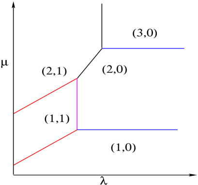
Figure 1: Schematic phase-diagram showing preferred particle distribution in $\mu$-$\lambda$ plane for $\delta=0$. The pairs of numbers $(n_{1},n_{2})$ denotes the particle numbers of the two species at each site.

The MI phase diagram for $\delta=0$ is shown in Fig. 1. We note from Eq. 16 that the boundary between MI phase $(1,0)$ and $(1,1)$ is determined by $\mathcal{E}_{10}=\mathcal{E}_{11}$ leading to the condition $\mu=\Omega+\lambda U$. Similarly, the boundary between $(1,0)$ and $(2,0)$ phases is determined by the condition $\mu=-\Omega+U$ while that between the $(1,1)$ and $(2,0)$ phases is given by $\lambda U=-2\Omega+U$.

For finite $\delta$, the energy of different Mott phases are determined by Eqs. 5, 9 and 15. Using these equations, we find the ground state numerically as function of $\mu$ and $\lambda$ for several representative values of $\Omega$ and $\delta$ as shown in Fig. 2. We note that the main effect of $\delta$ is to smoothen out the phase boundary between the phases and to realize a MI ground which a linear superposition of states with different $n_{1}$ and $n_{2}$ with a fixed $n=n_{1}+n_{2}$. For example, the ground state with $n=1$ in Fig. 2 is a linear superposition of the states $(1,0)$ and $(0,1)$. The overlap of a state $(n_{1},n_{2})$ with the ground state with $n=n_{1}+n_{2}$ depends on the precise values of $\delta$ and $\Omega$.

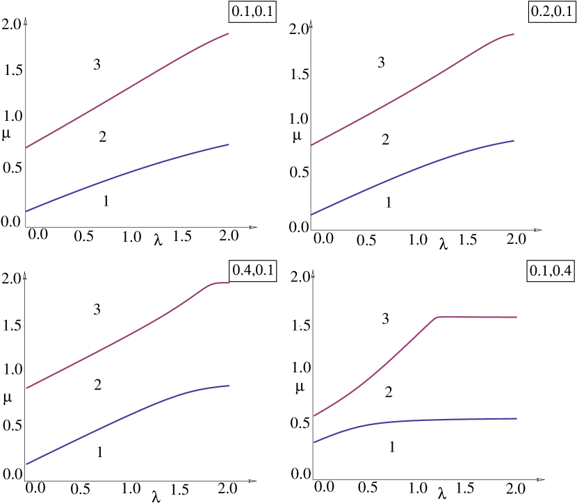
Figure 2: Schematic phase-diagram of the MI phase showing in the $\mu$-$\lambda$ plane for finite $\Omega$ and $\delta$. The numbers $1$, $2$, and $3$ denotes the total boson number $n$ at a given regime. The pair of in the box for each panel denote the values of $(\Omega,\delta)$ for which the phase diagram has been drawn.

II.2 Momentum distribution in the MI phase

In this section, we shall compute the momentum distribution of the Green function in the Mott phase for which $n=1$. The calculations can be generalized to any $n$ in a straightforward manner; however this requires handling quite complicated algebra which we refrain from in this work.

First, let us consider the Green function of the bosons in the MI phase in the atomic limit. For $n=1$, the Green function is a $2\times 2$ matrix given by

$$G_{0}(\tau,\tau^{\prime})=\left(\begin{array}[]{cc}\langle\mathcal{T}b^{\dagger}_{1}(\tau)b_{1}(\tau^{\prime})\rangle&\langle\mathcal{T}b^{\dagger}_{1}(\tau)b_{2}(\tau^{\prime})\rangle\\ \langle\mathcal{T}b^{\dagger}_{2}(\tau)b_{1}(\tau^{\prime})\rangle&\langle\mathcal{T}b^{\dagger}_{2}(\tau)b_{2}(\tau^{\prime})\rangle\end{array}\right)$$ (19)

To compute the Green function, we first consider the eigenenergies of $H_{\rm Mott}$. These are obtained by diagonalizing $E_{n}$ for the $n$ particle sector; for computing the zero-temperature Green function for the $n=1$, sector, we shall need the expressions of these energies for $n=1$ and $n=2$ sectors. For $n=1$, let us denote these energies by $\mathcal{E}^{1}_{1}$ and $\mathcal{E}^{1}_{2}$ with $\mathcal{E}^{1}_{1}<\mathcal{E}^{1}_{2}$. it can be easily seen from Eq. 5, that the corresponding eigenstates $|\mathcal{E}^{1}_{1}\rangle$ and $|\mathcal{E}^{1}_{2}\rangle$ are related to the states $|1,0\rangle$ and $|0,1\rangle$ by

$$\left(\begin{array}[]{c}|\mathcal{E}^{1}_{1}\rangle\\ |\mathcal{E}^{1}_{2}\rangle\end{array}\right)=\left(\begin{array}[]{cc}u_{1}&v_{1}\\ u_{2}&v_{2}\end{array}\right)\left(\begin{array}[]{c}|1,0\rangle\\ |0,1\rangle\end{array}\right)$$ (26)

where $v_{1}=u_{2}=\delta/{\mathcal{D}}$, and $u_{1}=v_{2}=-i(\Omega+\sqrt{\delta^{2}+\Omega^{2}})/{\mathcal{D}}$ where ${\mathcal{D}}=[\delta^{2}+(\Omega^{2}+\sqrt{\delta^{2}+\Omega^{2}})]^{1/2}$. Similarly for the $n=2$ sectors, we denote the eigenenergies and corresponding eigenfunctions of $H_{\rm Mott}$ by ${\mathcal{E}}_{1,2,3}^{2}$ and $|{\mathcal{E}}_{1,2,3}^{2}\rangle$ respectively. From Eq. 9, we find that the states $|{\mathcal{E}}_{1,2,3}^{2}\rangle$ are related to $|1,1\rangle$, $|2,0\rangle$, and $|0,2\rangle$ by

$$\left(\begin{array}[]{c}|1,1\rangle\\ |2,0\rangle\\ |0,2\rangle\end{array}\right)=\left(\begin{array}[]{ccc}x_{1}&y_{1}&z_{1}\\ x_{2}&y_{2}&z_{2}\\ x_{3}&y_{3}&z_{3}\end{array}\right)\left(\begin{array}[]{c}|\mathcal{E}^{2}_{1}\rangle\\ |\mathcal{E}^{2}_{2}\rangle\\ |\mathcal{E}^{2}_{3}\rangle\end{array}\right)$$ (36)

where the expressions of $x_{i}$, $y_{i}$ and $z_{i}$ can be found by diagonalizing the energy functional $E_{2}$ (Eq. 9). These coefficients are found numerically in the present work for finite $\delta$. Here we note that $x_{i}$, $y_{i}$ and $z_{i}$ are imaginary for $i=2,3$ and real for $i=1$. Using these expressions, a straightforward calculation following Ref. dupuis1, yields the atomic limit Green functions as

$$G^{0}_{11}(iw)=-\frac{|u_{1}|^{2}}{{\mathcal{E}}^{1}_{1}-iw}+\sum^{3}_{j=1}\frac{T^{j}_{11}}{\mathcal{E}^{2}_{j}-{\mathcal{E}}^{1}_{1}-iw},$$

$$G^{0}_{12}(iw)=-\frac{u^{*}_{1}v_{1}}{{\mathcal{E}}^{1}_{1}-iw}+\sum^{3}_{j=1}\frac{T^{j}_{12}}{\mathcal{E}^{2}_{j}-{\mathcal{E}}^{1}_{1}-iw},$$

$$G^{0}_{21}(iw)=-\frac{u_{1}v^{*}_{1}}{{\mathcal{E}}^{1}_{1}-iw}+\sum^{3}_{j=1}\frac{T^{j}_{21}}{\mathcal{E}^{2}_{j}-{\mathcal{E}}^{1}_{1}-iw},$$

$$G^{0}_{22}(iw)=-\frac{|v_{1}|^{2}}{{\mathcal{E}}^{1}_{1}-iw}+\sum^{3}_{j=1}\frac{T^{j}_{22}}{\mathcal{E}^{2}_{j}-{\mathcal{E}}^{1}_{1}-iw},$$ (37)

where $i\omega$ denotes Matsubara frequency and $T^{j}_{ab}$, for $j=1,2,3$ and $a,b=1,2$ are given by

$$T^{1}_{11} = 2|u_{1}|^{2}|x_{2}|^{2}+\sqrt{2}u_{1}v^{*}_{1}x^{*}_{1}x_{2}+\sqrt{2}u^{*}_{1}v_{1}x_{1}x^{*}_{2}$$

$$+|v_{1}|^{2}|x_{1}|^{2},$$

$$T^{1}_{22} = |u_{1}|^{2}|x_{1}|^{2}+\sqrt{2}u_{1}v^{*}_{1}x^{*}_{1}x_{3}+\sqrt{2}u^{*}_{1}v_{1}x_{1}x^{*}_{3}$$

$$+2|v_{1}|^{2}|x_{3}|^{2},$$

$$T^{1}_{21} = T_{12}^{1\ast}=\sqrt{2}|u_{1}|^{2}x^{*}_{2}x_{1}+u_{1}v^{*}_{1}|x_{1}|^{2}$$ (38)

$$+\sqrt{2}|v_{1}|^{2}x^{*}_{1}x_{3}+2v^{*}_{1}u_{1}x^{*}_{2}x_{3},$$

and $T_{ab}^{2}$ and $T_{ab}^{3}$ are obtained by replacing all $x_{i}$s in the expression of $T_{ab}^{1}$ by $y_{i}$ and $z_{i}$ respectively. Note that, when analytically continued to real frequencies using the prescription $i\omega\to\omega+i\epsilon$, $G^{0}_{ij}(\omega)$ is imaginary for $i\neq j$ and real for $i=j$ for $\epsilon=0$.

The Green functions obtained in Eq. 37 can be easily understood as follows. Each term $G^{0}_{ab}$ receives contribution from a hole branch which corresponds to removal of one particle from the Mott state which cost an energy ${\mathcal{E}}_{1}^{1}$ in the atomic limit. The other terms represents contribution from the different possible particle branches which corresponds to addition of a particle over the ground state with $n=1$ and cost energies $\mathcal{E}^{2}_{j}-\mathcal{E}^{1}_{1}$ for $j=1,2,3$. The poles of the Green functions occur at these particle and hole excitation energies.

To obtain the Green function for finite nearest-neighbor terms $t_{a}$ and $\gamma$, we follow the procedure introduced in Ref. dupuis1, . First, we define the bosonic fields as $\psi_{ai}(\tau)\equiv\psi_{a}({\bf r_{i}},\tau)$, where $a=1,2$, $i$ denote the site index of the optical lattice and $\tau$ is the imaginary time. In terms of these fields, the nearest-neighbor hopping and spin-orbit coupling terms given by Eqs. 2 and 3 can be written as

$$S_{0} = \int_{0}^{\beta}d\tau\sum_{\langle ij\rangle}\Big{[}\left(\psi^{\ast}_{1i}\psi_{2i}^{\ast}\right)\Lambda\left(\begin{array}[]{c}\psi_{1j}\\ \psi_{2j}\end{array}\right)+{\rm h.c}\Big{]}$$ (41)

$$\Lambda = \left(\begin{array}[]{cc}-t_{1}&i\gamma(\delta_{j,i\pm{\hat{y}}}+(-1)^{a}i\delta_{j,i\pm{\hat{x}}})\\ -i\gamma(\delta_{j,i\pm{\hat{y}}}-(-1)^{a}i\delta_{j,i\pm{\hat{x}}})&-t_{2}\end{array}\right),$$ (44)

where we have omitted the $\tau$ index of the boson fields for clarity, $\beta=1/k_{B}T$ is the inverse temperature and $k_{B}$ is the Boltzman constant which will be subsequently set to unity. We then write down the coherent state path integral for the bosons and decouple the nearest-neighbor hopping and spin-orbit coupling terms by two Hubbard-Stratonovitch fields $\Delta_{i}(\tau)=[\Delta_{1i}(\tau)\Delta_{2i}(\tau)]^{T}$ and so that the partition function of the bosons can be written as (with $\hbar=1$)

$$Z = \int{\mathcal{D}}\psi_{a}^{\ast}{\mathcal{D}}\psi_{a}{\mathcal{D}}\Delta_{a}e^{-S_{1}[\psi_{a}^{\ast},\psi_{a},\Delta_{a}]}$$

$$S_{1} = \int_{0}^{\beta}d\tau\Big{[}\sum_{ia}\Big{(}\psi_{ia}\partial_{\tau}\psi_{ia}-(\Delta_{i}^{\ast}\psi_{ia}+{\rm h.c})\Big{)}+H_{\rm Mott}$$ (45)

$$-\sum_{\langle ij\rangle}\Delta_{i}^{\ast}\Lambda^{-1}\Delta_{j}\Big{]}$$

Next, we introduce a second Hubbard-Stratonovitch field $\Phi_{i}(\tau)=[\Phi_{1i}(\tau),\Phi_{2i}(\tau)]^{T}$ to decouple the last term in $S_{1}$ (Eq. 45). This leads to

$$Z = \int{\mathcal{D}}\psi_{a}^{\ast}{\mathcal{D}}\psi_{a}{\mathcal{D}}\Delta_{a}{\mathcal{D}}\Phi_{a}e^{-S_{2}[\psi_{a}^{\ast},\psi_{a},\Delta_{a},\Phi_{a}]}$$

$$S_{2} = \int_{0}^{\infty}d\tau\Big{[}\sum_{ia}\Big{(}\psi_{ia}\partial_{\tau}\psi_{ia}+[\Delta_{i}^{\ast}(\Phi_{ia}-\psi_{ia})+{\rm h.c}\Big{)}$$ (46)

$$+H_{\rm Mott}-\sum_{\langle ij\rangle}\Phi_{i}^{\ast}\Lambda\Phi_{j}\Big{]}$$

We note that the field $\Phi_{ia}(\tau)$ have exactly the same correlators as the original boson fields dupuis1 . With this observation, we integrate out the fields $\Delta_{ia}(\tau)$ and $\psi_{ia}(\tau)$ to obtain an effective action in terms of the field $\Phi_{ia}(\tau)$. The details of the procedure for doing so is elaborated in Ref. dupuis1, . After some algebra, the quadratic and the quartic part of the resultant action is obtained to be

$$S^{(2)}_{\rm eff} = \frac{1}{\beta}\sum_{\omega_{n};a,b}\int\frac{d^{2}k}{(2\pi)^{2}}\Phi_{a}^{\ast}(k)\left[-G^{0-1}(\omega_{n})\right.$$ (47)

$$\left.+\Lambda({\bf k})\right]_{ab}\Phi_{b}(k)$$

$$S^{(4)}_{\rm eff} = \frac{g}{2}\int_{0}^{\beta}d\tau\int d^{2}x\left|\sum_{a}\Phi_{a}^{\ast}(r)\Phi_{a}(r)\right|^{2}$$ (48)

where $G^{0}$ denotes the boson Green functions in the atomic limit, $k\equiv(\omega_{n};{\bf k})$, $r\equiv(\tau;{\bf x})$, and $\Lambda({\bf k})$ is given by

$$\Lambda({\bf k}) = -2\left(\begin{array}[]{cc}t_{1}(\cos k_{x}+\cos k_{y})&\gamma(i\sin k_{x}+\sin k_{y})\\ \gamma(-i\sin k_{x}+\sin k_{y})&t_{2}(\cos k_{x}+\cos k_{y})\end{array}\right).$$ (51)

In what follows we shall analyze $S^{(2)}_{\rm eff}$ and $S^{(4)}_{\rm eff}$ within mean-field theory to obtain the properties of MI and SF phases of the bosons. We shall neglect all high order terms in the boson effective action which can be shown to be irrelevant in the low-energy, low-momentum limit dupuis1 .

In the MI phase, $\langle\Phi_{a}(k)\rangle=0$ and the boson action, within mean-field theory, is given by $S_{\rm eff}^{(2)}$. The momentum distribution of the bosons in the MI phase at zero temperature can then obtained from the boson Green function $G_{\rm eff}(k)=\left[-G^{0-1}(\omega)+\Lambda({\bf k})\right]^{-1}$ as

$$n({\bf k}) = \int_{-\infty}^{0}\frac{d\omega}{2\pi}{\rm Tr}\,G_{\rm eff}(k)$$ (53)

where ${\rm Tr}$ denotes matrix trace and we have used $\omega_{n}\to\omega+i\epsilon$ for analytic continuation to real frequencies. To evaluate the integral, we note that the integrand ${\rm Tr}\,G_{\rm eff}(k)$ is invariant under an unitary transformation; consequently $n({\bf k})$ in Eq. 53 can be written as $n({\bf k})=\int_{-\infty}^{0}d\omega{\rm Tr}\,G^{d}_{\rm eff}(k)/(2\pi)$ where $G^{d}_{\rm eff}(k)$ is obtained by diagonalizing $G_{\rm eff}(k)$ via an unitary transformation and can be written as

$$G_{\rm eff}^{d}(k)=\prod_{i=1}^{n_{band}}\frac{{\mathcal{A}}_{i}(\omega;{\bf k})}{\left[\omega-\epsilon_{i}({\bf k})\right]},$$ (54)

where $\epsilon_{i}({\bf k})$ are the band energies which are obtained as solution of ${\rm Det}[G^{-1}_{\rm eff}(\epsilon;{\bf k})]=0$, ${\mathcal{A}}_{i}(\omega,{\bf k})$ are the residue of the Green function at the pole $\omega=\epsilon_{i}({\bf k})$ which has to be determined numerically for finite $\delta$, and $n_{band}$ is the total number of such bands. The equation for determining these bands can be written using Eq. 37, LABEL:endisp1, and 47 as

$$\{[G_{0}^{-1}(\epsilon)]_{11}+2t_{1}(\cos(k_{x})+\cos(k_{y}))\}$$

$$\times\{[G_{0}^{-1}(\epsilon)]_{22}+2t_{2}(\cos(k_{x})+\cos(k_{y}))\}$$

$$=4\sin^{2}(k_{y})\gamma^{2}+\left[2\gamma\sin(k_{x})+[G_{0}^{{}^{\prime}-1}(\epsilon)]_{12}\right]^{2}$$ (55)

where we have used the fact that $[G_{0}^{-1}(\epsilon)]_{12}=[G_{0}^{-1}(\epsilon)]_{21}^{\ast}$ and $[G_{0}^{{}^{\prime}-1}(\epsilon)]_{12}=-i[G_{0}^{-1}(\epsilon)]_{12}$. We note that for finite $\delta$, $[G_{0}^{-1}(\epsilon)]_{12}\neq 0$. Consequently, Eq. 55 is invariant under $k_{y}\to-k_{y}$ but not under $k_{x}\to-k_{x}$; thus the energy bands satisfy $\epsilon_{i}(k_{x},k_{y})=\epsilon_{i}(k_{x},-k_{y})\neq\epsilon_{i}(-k_{x},k_{y})$. A plot of the highest negative and the lowest positive energy bands for representative values of parameters is shown in Fig. 3. The plot clearly indicates two minima at $k_{y}=\pm k_{y}^{0}=\pm k_{0}$ and $k_{x}=k_{0}$. Also, we find that for the above-mentioned parameter values $n_{band}=8$; there are two bands with negative and six bands with positive energies.

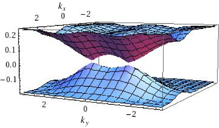
Figure 3: The highest hole and the lowest particle bands of the bosons for $\lambda=0.4,\,\Omega=0.01U,\,\delta=0.005U,\,t=0.02U,\,\gamma=0.049U,\,\mu=0.175U,\,{\rm and}\,\eta=0.5$.

To compute $n({\bf k})$, we note that the contribution to $n({\bf k})$ comes from the bands for which $\epsilon({\bf k})\leq 0$. Labeling such energy bands as $\epsilon^{-}_{i}({\bf k})$ and denoting their number by $n_{band}^{-}$, one obtains the momentum distribution as

$$n({\bf k}) = \sum_{i=1}^{n^{-}_{band}}{\mathcal{A}}_{i}(\epsilon_{i}({\bf k});{\bf k})\prod_{j=1}^{n_{band}}\frac{(1-\delta_{ij}){\mathcal{A}}_{j}(\epsilon_{i}({\bf k});{\bf k})}{[\epsilon_{j}({\bf k})-\epsilon_{i}^{-}({\bf k})]}$$

where the sum extends over all bands with $\epsilon_{i}\leq 0$.

The plot of $n({\bf k})$ is shown in Fig. 4. As expected, we find $n({\bf k})$ develops precursor peaks as one approaches the SI transition point by increasing $t_{a}$ and $\gamma$. This feature of $n({\bf k})$ can be easily understood from Eq. II.2 and Fig. 3 by noting the following points. First, the energy bands are independent of ${\bf k}$ for $t_{a}=\gamma=0$ (atomic limit) leading to a flat $n({\bf k})$. Second, as we approach the SI transition, the gap between the highest band with $\epsilon_{i}({\bf k})<0$ and the lowest band with $\epsilon_{i}({\bf k})>0$ decreases at special points $(k_{x}^{0},\pm k_{y}^{0})$ in the Brillouin zone. This results in peaks of $n({\bf k})$ at these points as we approach the SI transition. These peaks are precursors to the SI transition at which the bands touch; the position of these precursor peaks depend on the ratio $\gamma/t_{1}$ (for a fixed $\eta$) and can be continually tuned from $(\pi/2,\pm\pi/2)$ to $(0,0)$ as $\gamma/t_{1}$ is decreased. Note that since $\epsilon_{i}(k_{x},k_{y})=\epsilon_{i}(k_{x},-k_{y})$, both $(k_{x}^{0},k_{y}^{0})$ and $(k_{x}^{0},-k_{y}^{0})$ correspond to the peak position; however, since $\epsilon_{i}(k_{x},k_{y})\neq\epsilon_{i}(-k_{x},k_{y})$ for finite $\delta$, $n({\bf k})$ need not (and does not) have a peak at $(-k_{x}^{0},k_{y}^{0})$ unless $\delta=0$. Numerically, we find $k_{x}^{0}=k_{y}^{0}=k_{0}$ for all the parameter range we study. Thus our work demonstrates that the key effect of the spin-orbit coupling is to shift these precursor peaks from $(0,0)$ to finite momenta $(k_{0},\pm k_{0})$ in the Brillouin zone. In the next section, we shall investigate the effect of this shift on the SI transition point.

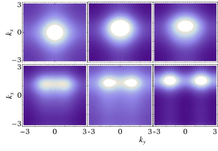
Figure 4: The momentum distribution of the bosons in the MI phase showing the precursor peaks moving from center of the Brillouin zone to $(\pi/2,\pm\pi/2)$ with increasing $\gamma/t$. The plots correspond to $\mu=0.2U$ and have (from top left to bottom right) $(t,\gamma)$ to be $(0.03,0)$, $(0.03,0.02)$, $(0.025,0.025)$, $(0.015,0.04)$, $(0.01,0.045)$, and $(0.0,0.048)$ in units of $U$. The lighter colors indicate larger values of $n({\bf k})$. All other parameter values are same in Fig 3.

III Superfluid-Insulator transition

In this section, we shall analyze the SI transition for two species bosons with spin-orbit coupling. We use the strong coupling Green function developed in Sec. II.2 to construct an effective low-energy critical theory for the transition. This is followed by the analysis of the critical theory in Sec. III.2.

III.1 Critical Theory

In this section, we analyze the critical theory of the superfluid-insulator transition using $S^{(2)}_{\rm eff}$ and $S^{(4)}_{\rm eff}$ (Eqs. 47 and 48) derived in Sec. II.2. These terms provide the microscopic basis for construction of an effective Landau-Ginzburg functional for the MI-SF transition. The analytical calculations in this section will be carried out for $\delta=0$ for simplicity; however, we shall provide qualitative statements for $\delta\neq 0$ case at the end of this section.

We consider approaching the critical point from the MI side. For $\delta=0$, the on-site Green function $G^{0}$ is diagonal with the elements $G_{11}^{0}$ and $G_{22}^{0}$ given by

$$G_{11}^{0}(\omega) = \frac{-1}{\omega+E_{0}}+\frac{2}{\omega+E_{0}-U},\quad G_{22}^{0}(\omega)=\frac{1}{\omega-E_{1}},$$

$$E_{0} = \mu+\Omega,\quad E_{1}=\mu-\Omega-\lambda U.$$ (57)

This allows us to write $(G^{0})^{-1}$ as a diagonal matrix

$$(G^{0})^{-1} = \left(\begin{array}[]{cc}F_{1}(\omega)&0\\ 0&F_{2}(\omega)\end{array}\right)$$ (60)

$$F_{1}(\omega) = \omega+E_{0}-\frac{2U(\omega+E_{0})}{\omega+E_{0}+U},\quad F_{2}(\omega)=\omega-E_{1}.$$

Using Eq. 60, one can write the effective action $S^{(2)}_{\rm eff}(\delta=0)$ as

$$S^{(2)}_{\rm eff}(\delta=0) = -\sum_{a,b=1,2}\int\frac{d^{2}kd\omega}{(2\pi)^{3}}\Phi_{a}^{\ast}(k)G^{-1}(k)\Phi_{b}(k)$$

$$G^{-1}(k) = \left(\begin{array}[]{cc}F_{1}(\omega)+2t[\cos(k_{x})+\cos(k_{y})]&2\gamma[i\sin(k_{x})+\sin(k_{y})]\\ 2\gamma[-i\sin(k_{x})+\sin(k_{y})]&F_{2}(\omega)+2t[\cos(k_{x})+\cos(k_{y})]\end{array}\right)$$ (63)

where $k\equiv(\omega,{\bf k})$. Diagonalizing $G^{-1}(k)$, we find the two eigenvalues to be

$$\lambda_{\pm} = \frac{1}{2}\Big{[}F_{+}(\omega)+4t[\cos(k_{x})+\cos(k_{y})]$$ (64)

$$\pm\sqrt{F_{-}^{2}(\omega)+16\gamma^{2}[\sin^{2}(k_{x})+\sin^{2}(k_{y})]}\Big{]}$$

where $F_{\pm}(\omega)=F_{1}(\omega)\pm F_{2}(\omega)$. Thus the quadratic part of the effective action of the bosons can be written as

$$S^{(2)}_{\rm eff}(\delta=0) = -\sum_{a=\pm}\int\frac{d^{2}kd\omega}{(2\pi)^{3}}\Phi_{a}^{\ast}(k)\lambda_{a}(k)\Phi_{a}(k)$$ (65)

where $\Phi_{+(-)}=\alpha_{1}^{+(-)}\Phi_{1}+\alpha_{2}^{+(-)}\Phi_{2}$ are linear combinations of the fields $\Phi_{1}$ and $\Phi_{2}$ and $\alpha_{1,2}^{\pm}$ are the components of eigenfunctions of $G^{-1}(k)$ corresponding to eigenvalues of $\lambda_{\pm}$ given by

$$\frac{\alpha_{2}^{\pm}}{\alpha_{1}^{\pm}} = -\frac{F_{1}(\omega)+2t[\cos(k_{x})+\cos(k_{y})]-\lambda_{\pm}(k)}{2\gamma[i\sin(k_{x})+\sin(k_{y})]}$$ (66)

At the quantum critical point, for $\delta=0$, $\lambda_{-}(\omega=0,\pm k_{x}=\pm k_{y}=k_{0})$ touches zero which signifies the destabilization of the MI phase. The expression for $k_{0}$ and the critical values of $t$ and $\gamma$ at which this happens can be found from the conditions $\lambda_{-}(\omega=0,\pm k_{x}=\pm k_{y}=k_{0})=0$ and $\partial\lambda_{-}(\omega=0,\pm k_{x}=\pm k_{y}=k_{0})/\partial k_{0}=0$ and yields (with $F_{\pm}\equiv F_{\pm}(\omega=0)$)

$$F_{+}+8t\cos(k_{0}) = \sqrt{F_{-}^{2}+32\gamma^{2}\sin^{2}(k_{0})}$$

$$\sin(k_{0})\left(\cos(k_{0})+\frac{F_{+}t}{4\gamma^{2}+8t^{2}}\right) = 0$$ (67)

Eqs. 67 provide us the position of the critical point and allows to find $\gamma_{c}/U$ ($t_{c}/U$) and $k_{0}$ for any given $t/U$ ($\gamma/U$), $\mu/U$, $\lambda$, and $\Omega/U$. The basic features of the solution to Eq. 67 is as follows. For $\gamma=0$, the only solution of Eq. 67 is $k_{0}=0$ and $t_{c}^{(1)}=(|F_{-}|-F_{+})/8$. As we turn of a finite $\gamma$, another possible solution emerges at $k^{\prime}_{0}=\arccos(F_{+}t_{c}^{(2)}(\gamma)/(4\gamma^{2}+8[t_{c}^{(2)}(\gamma)]^{2})$ where $t_{c}^{(2)}$ is the solution of $F_{+}+8t_{c}^{(2)}(\gamma)\cos(k^{\prime}_{0})=\sqrt{F_{-}^{2}+32\gamma^{2}\sin^{2}(k^{\prime}_{0})}$. Depending on the chosen $\mu$, $\Omega$, and $\lambda$, there is a critical value of $\gamma=\gamma_{0c}$, at which $t_{c}^{(2)}(\gamma)\leq t_{c}^{1}$. At this value of $\gamma_{0c}$, $k_{0}$ shifts to a non-zero value $k^{\prime}_{0}$. A similar behavior may be inferred by choosing a fixed $t$ and by slowing increasing $\gamma$ to reach the transition. In particular we note that in such cases, for $t=0$, $k_{0}=\pi/2$ and $\gamma_{c}=\sqrt{F_{1}F_{2}/8}$. A plot of the phase-diagram based on Eq. 67 is shown in Fig. 5. The top left panel of Fig. 5 shows the MI-SF phase diagram in the $\mu-\gamma$ plane for specific $t$ while the top right panel exhibit the phase diagram in the $t-\mu$ plane for specific $\gamma$. These plots are qualitatively similar to their mean-field counterparts in Fig. 7 and exhibit reentrant SI transition as a function of $\gamma$ for any non-zero $t$. The bottom panels of Fig. 5 shows the phase diagrams for finite $\delta$ (computed numerically starting from the expression of $G_{0}$ for finite $\delta$ in Eq. 37 and using the method outlined in this section) which are seen to be qualitatively similar to their $\delta=0$ counterparts. The left panel of Fig. 6 shows a plot of $k_{0}$ as a function of $t_{c}(\mu)$ for several representative values of $\gamma$ with $\lambda=0.4$, and $\Omega=0.01U$. We find that for small $\gamma$, there is a finite range of $t_{c}$ for which the transition takes place at $k_{0}=0$. The width of this region shrinks with increasing $\gamma$ and beyond a critical $\gamma=\gamma^{\prime}_{c}$, the transition always takes place with finite $k_{0}$. For $\lambda=0.4$ and $\Omega=0.01U$, we find $\gamma^{\prime}_{c}\simeq 0.033U$ as can be seen from the left panel of Fig. 6.

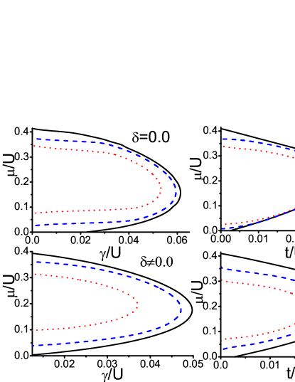
Figure 5: The phase boundary in the $\mu-\gamma$ (left panels) and $\mu-t$ plane (right panels) for $\eta=1$, and $\Omega=0.01U$ as obtained from the strong-coupling analysis. The top panels have $\delta=0$ while the bottom panels have $\delta=0.005U$. The values of $t$ for the left panels corresponding to different lines are $t/U=0.0$ (black solid), $t/U=0.01$ (blue dashed), $0.02$ (red dotted). For the right panels, $\gamma/U=0$ (black solid line), $0.03$ (blue dashed line) and $0.04$ (red dotted line).

The critical theory for the MI-SF transition can now be constructed in terms of the low-energy excitations around $\omega=0$ and $k=k_{0}$ which can be described by a set of bosonic fields $\varphi_{i}(k)$ around each of these minimum. For $n$ such minima at $k_{0}\equiv k_{0}^{i}$ where $i=1..n$, one expresses the field $\Phi_{-}=\Phi_{-}(\omega=0,{\bf k}=k_{0}^{i})+\varphi_{i}(k)$ and obtain the quadratic action

$$S_{2}^{\rm cr} = -\int\frac{d^{2}kd\omega}{(2\pi)^{3}}\sum_{i=1}^{n}\varphi_{i}^{\ast}(k)\left(K_{0}\omega+K_{1}\omega^{2}-v^{2}|{\bf k}|^{2}\right)\varphi_{i}(k)$$

$$K_{0} = \frac{\partial\lambda_{-}}{\partial\omega}\Big{|}_{\omega=0,{\bf k}=k_{0}^{i}}=\frac{1}{2}\Big{[}F^{\prime}_{+}(0)-\frac{F_{-}(0)F^{\prime}_{-}(0)}{F_{+}(0)+8t\cos(k_{0}^{i})}\Big{]}$$

$$K_{1} = \frac{1}{2}\frac{\partial^{2}\lambda_{-}}{\partial\omega^{2}}\Big{|}_{\omega=0,{\bf k}=k_{0}^{i}}=\frac{1}{4}\Big{[}F^{{}^{\prime\prime}}_{+}(0)$$

$$-\frac{F_{-}^{{}^{\prime}2}(0)+F^{{}^{\prime\prime}}_{-}(0)F_{-}(0)}{F_{+}(0)+8t\cos(k_{0}^{i})}+\frac{[F^{\prime}_{-}(0)F_{-}(0)]^{2}}{[F_{+}(0)+8t\cos(k_{0}^{i})]^{3}}\Big{]}$$

$$v^{2} = \frac{1}{2}\frac{\partial^{2}\lambda_{-}}{\partial(k_{0}^{i})^{2}}\Big{|}_{\omega=0,{\bf k}=k_{0}^{i}}=-2\Big{[}t\cos(k_{0}^{i})$$ (68)

$$+\frac{8\gamma^{2}\cos(2k_{0}^{i})}{F_{+}(0)+8t\cos(k_{0}^{i})}+\frac{64\gamma^{4}\sin^{2}(2k_{0}^{i})}{[F_{+}(0)+8t\cos(k_{0}^{i})]^{3}}\Big{]}$$

where ^′ denotes differentiation with respect to $\omega$. From Eq. 68, we find that the critical theory has dynamical critical exponent $z=2$ except for special points at which $K_{0}=0$ leading to $z=1$. In usual MI-SF transition this point appears to be at the tip of the MI lobe. Here we find a line of such $z=1$ transitions in the $t-\gamma$ plane as shown in the right panel of Fig. 6 for representative values $\delta=0$, $\lambda=0.4$, $\eta=1$, and $\Omega=0.01U$.

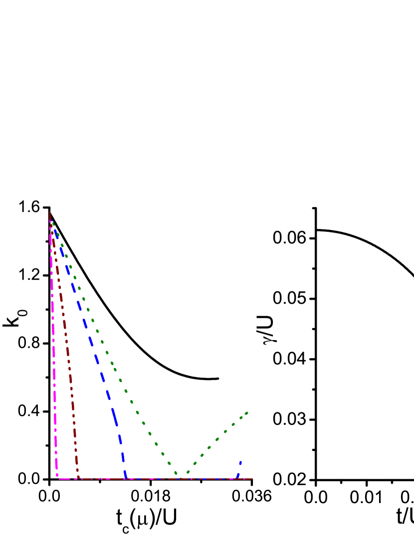
Figure 6: Left panel: Plot of $k_{0}$ against $t_{c}(\mu)$ for $\gamma/U=0.01$(pink dash dot dotted), $0.02$ (yellow dash dotted ), $0.03$ (blue dotted), $0.0333$ (green dashed) and $0.04$(black solid) line. Right panel: Plot of the line with $z=1$ quantum phase transition in the $\gamma-t$ plane as obtained from solution of $K_{0}=0$.For all plots $\delta=0$, $\lambda=0.4$, $\eta=1$, and $\Omega=0.01U$.

The structure of the quadratic part of the critical action found in Eq. 68 remains qualitatively similar for $\delta\neq 0$ except for two differences. The first difference in the effective action comes from the fact that the number of minima is halved due to the lifting of $k_{x}\to-k_{x}$ symmetry as discussed in Sec. II.2 while the second difference stems from the fact that $v_{x}\neq v_{y}$ for $\delta\neq 0$ leading to an anisotropic dispersion of the critical theory. Consequently, the critical action $S_{2}$ now has the form

$$S_{2}^{\rm cr;\delta\neq 0} = -\int\frac{d^{2}kd\omega}{(2\pi)^{3}}\sum_{i=1}^{n}\varphi_{i}^{\ast}(k)\left(K_{0}\omega+K_{1}\omega^{2}\right.$$ (69)

$$\left.-v_{x}^{2}k_{x}^{2}-v_{y}^{2}k_{y}^{2}\right)\varphi_{i}(k)$$

The positions of the $z=1$ line in the $\mu-\gamma$ plane also changes. However, rest of the features remain the same. In Sec. III.2, we shall analyze the critical theory in details and show that the MI-SF transition at $t/\gamma=0$ is unconventional in the sense that it is accompanied by the emergence of an additional gapless mode at criticality.

III.2 Analysis of the critical theory

Having established the analytical form for $S_{2}^{\rm cr}$ for $\delta=0$, we shall now analyze the effective Landau-Ginzburg theory for the transition. The quadratic part of the effective action remains the same as in Eq. 68. Our analysis shall hold for $\delta\neq 0$ as well; in this case Eq. 68 shall be substituted by Eq. 69. In this section, we shall not bother with microscopic calculation; instead we shall analyze the critical theory from the symmetry perspective as done, for example, in Ref. balents1, , for small $t/\gamma$ where the minima of $G^{-1}(k)$ occurs at non-zero ${\bf k}_{0}^{\pm}=(k_{0},\pm k_{0})$. In the presence of two such minima, the bosonic field can be written as

$$\Phi_{-}({\bf r},t)=\varphi_{1}({\bf r},t)e^{i{\bf k_{0}^{+}}\cdot{\bf r}}+\varphi_{2}({\bf r},t)e^{i{\bf k_{0}^{-}}\cdot{\bf r}}.$$ (70)

Substitution of Eq. 70 in Eq. 65 and subsequent expansion in $\omega$ and ${\bf k}$ (around ${\bf k}_{0}^{\pm}$) leads to Eq. 68 with $n=2$.

To obtain the quartic action, one can in principle substitute Eq. 70 in Eq. 48, average over the fast oscillating components involving various powers of $\cos({\bf k}_{0}^{\pm}\cdot{\bf r})$ and $\sin({\bf k}_{0}^{\pm}\cdot{\bf r})$ which appears in the expression of $S_{4}$, and obtain an effective critical action in terms of $\varphi_{1,2}$. However, such an averaging proves to be tricky when $\pi/(k_{0}^{\pm}a)$ do not turn out to be a small integer since one may have to sum over an arbitrary large number of lattice sites for achieving a proper averaging sinha1 . Also, for irrational $k_{0}^{\pm}$, such an averaging procedure is ill-defined. For our case, since $k_{0}^{\pm}$ is a continuous function of $t/\gamma$, we adopt a symmetry-based general method for deriving the fourth order term in the action.

The symmetry based derivation of the effective action relies on the fact that an effective low-energy Landau-Ginzburg action describing a phase transition must be invariant under the projective symmetry group (PSG) transformation of its underlying lattice balents1 . The elements of PSG for a square lattice are translation by a lattice vector along $x$ and $y$ ($T_{x}$ and $T_{y}$), rotation about the $z$ axis by $\pi/2$ ($R_{\pi/2}$), and reflection about $x$ and $y$ axes ($P_{x}$ and $P_{y}$). Following the method derived in Ref. balents1, and using Eq. 70, we find that under these transformation the bosonic field $\varphi({\bf r},t)$ transforms as

$$T_{x}:\varphi_{1}\rightarrow e^{ik_{0}a}\varphi_{1},\quad\varphi_{2}\rightarrow e^{-ik_{0}a}\varphi_{2},$$

$$T_{y}:\varphi_{1}\rightarrow e^{ik_{0}a}\varphi_{1},~{}~{}~{}~{}\varphi_{2}\rightarrow e^{ik_{0}a}\varphi_{2},$$

$$R_{\pi/2}\varphi_{1}\rightarrow e^{2ik_{0}y}\varphi_{1},~{}~{}~{}~{}\varphi_{2}\rightarrow e^{2ik_{0}x}\varphi_{2}$$

$$P_{x}:\varphi_{1}\to\varphi_{2},\quad\varphi_{2}\to\varphi_{1}$$

$$P_{y}:\varphi_{1}\to\varphi_{2}^{\ast},\quad\varphi_{2}\to\varphi_{1}^{\ast}$$ (71)

To find the fourth order effective action consistent with Eq. 71, we first consider the case $t=0$ for which $k_{0}=\pi/2$. In this case, the most general form of the quartic action is

$$S_{4}^{\rm cr} = \frac{g}{2}\int d^{2}rdt\left[\left(|\varphi_{1}|^{2}+|\varphi_{2}|^{2}\right)^{2}+\eta_{0}(\varphi_{1}^{\ast}\varphi_{2}+{\rm h.c})^{2}\right]$$

where $\eta_{0}$ is a constant whose value will be determined later. Redefining the fields $\xi_{1(2)}=(\varphi_{1}+(-)\varphi_{2})/\sqrt{2}$, one gets

$$S_{4}^{\rm cr} = \frac{g}{2}\int d^{2}rdt\left[\left(|\xi_{1}|^{2}+|\xi_{2}|^{2}\right)^{2}+\eta_{0}(|\xi_{1}|^{2}-|\xi_{2}|^{2})^{2}\right]$$

For $\eta_{0}>0$, the ground state of $S_{4}^{\rm cr}$ and $S_{2}^{\rm cr}$ thus correspond to condensation of both the fields: $\xi_{1}=\xi_{1}^{0}$ and $\xi_{2}=\xi_{2}^{0}\exp(i\mu_{0})$. However, the relative phase $\mu_{0}$ between these two fields is not fixed by the $S_{4}^{\rm cr}$. Indeed, if we construct the eighth order term $S_{8}$ in the effective action, it will have a PSG allowed term $S_{8}=\lambda^{\prime}\int d^{2}rdt(\xi_{1}^{\ast}\xi_{2}+{\rm h.c})^{4}$ which will fix $\mu_{0}=m\pi/2$ for $\lambda^{\prime}<0$ and $\mu_{0}=(m+1/2)\pi/2$ for $\lambda^{\prime}>0$ where $m$ is an integer. Thus the effective phase mode characterized by the fluctuation of the relative phase $\mu_{0}$ is massive in the SF phase but is expected to become gapless when $\lambda^{\prime}\to 0$ due to irrelevance of $S_{8}$ at criticality. Consequently, we expect all transitions with $\eta_{0}>0$ to have an additional gapless mode in the critical region. To compute the value of $\eta_{0}$, we note that since $\pi/(k_{0}a)=2$, it is possible to compute the effective action $S_{4}^{\rm cr}$ by direct substitution of Eq. 70 in Eq. 48, followed by averaging over fast oscillating terms as shown in Ref. sinha1, . This procedure yields Eq. LABEL:act0 with $\eta_{0}=1$. Thus we find that for $t/\gamma=0$, the two-species bosons with spin-orbit coupling undergoes an unconventional phase transition at $\gamma=\gamma_{c}$ which are accompanied by emergence of an additional gapless mode at the transition balents1 . We note that this also implies that the vortices corresponding to any one of these fields $\varphi_{1}$ or $\varphi_{2}$ will have a fractional vorticity in the sense that a boson wavefunction would pick up a phase $\pi$ when moved around such a vortex balents1 . However, generating such vortices experimentally in present systems may turn out to be difficult.

For $t/\gamma\neq 0$ where $k_{0}\neq\pi/2$, we find that the only form of the effective action which is consistent with the PSG transformation has the form

$$S_{4}^{{}^{\prime}\rm cr} = \frac{g}{2}\int d^{2}rdt\left[\left(|\varphi_{1}|^{2}+|\varphi_{2}|^{2}\right)^{2}+\eta_{0}^{\prime}|\varphi_{1}|^{2}|\varphi_{2}|^{2}\right]$$

The value of $\eta^{\prime}_{0}$ is difficult to determine for arbitrary $k_{0}$; however, for certain values of $k_{0}$ which satisfies $k_{0}/(\pi a)\in Z$, one can determine $\eta^{\prime}_{0}$. In all such case we find $\eta^{\prime}_{0}\geq 0$. This indicates that for all $t/\gamma$, only one of the fields $\varphi_{1}$ or $\varphi_{2}$ condenses. Thus the MI-SF critical points for such finite $t/\gamma$ are conventional.

IV Mean-field Analysis

In this section, we use a Gutzwiller wavefunction to obtain the mean-field SI phase boundary for the system. The Gutzwiller variational wavefunction which we shall use is given by

$$|\psi_{i}\rangle = a_{i}|1,0\rangle_{i}+b_{i}|0,1\rangle_{i}+c_{i}|1,1\rangle_{i}+d_{i}|2,0\rangle_{i}$$

$$+e_{i}|0,2\rangle_{i}+f_{i}|0,0\rangle_{i},$$

$$|\Psi_{G}\rangle = \prod_{i}|\psi_{i}\rangle.$$ (75)

Note that for the purpose of charting out the phase diagram and for describing the SF phase near the SI transition point, it is not necessary to incorporate the higher number states since we expect these states to have very small overlap with the ground state of the system as can be checked by explicit numerical calculation. The variational energy of the system can be easily computed using Eqs. 2, 3 and 75 and yields

$$E = \langle\Psi_{G}|({\mathcal{H}}_{0}+{\mathcal{H}}_{1}|\Psi_{G}\rangle=E_{0}+E_{1}+E_{2}$$

$$E_{0} = \sum_{i}-(\mu+\Omega)|a_{i}|^{2}-(\mu-\Omega)|b_{i}|^{2}+(\lambda-2\mu)|c_{i}|^{2}$$

$$+(1-2\mu-2\Omega)|d_{i}|^{2}+(1-2\mu+2\Omega)|e_{i}|^{2}$$

$$+i\delta[b_{i}a^{*}_{i}-a_{i}b^{*}_{i}+\sqrt{2}c_{i}d^{*}_{i}-\sqrt{2}c^{*}_{i}d_{i}$$

$$+\sqrt{2}c^{*}_{i}e_{i}-\sqrt{2}c_{i}e^{*}_{i}],$$

$$E_{1} = -t_{1}\sum_{\langle{ij}\rangle}(\Delta_{i1}^{\ast}\Delta_{{j}1},+\eta\Delta_{i2}^{\ast}\Delta_{j2})+{\rm h.c.}$$

$$E_{2} = -\gamma\Big{[}\sum_{\langle{ij_{x}}\rangle}(\Delta_{i1}^{\ast}\Delta_{j_{x}2}-\Delta_{i2}^{\ast}\Delta_{j_{x}1})$$ (76)

$$+i\sum_{\langle ij_{y}\rangle}(\Delta_{i1}^{\ast}\Delta_{j_{y}2}+\Delta_{i2}^{\ast}\Delta_{j_{y}1})\Big{]}+{\rm h.c.}$$

where $\sum_{\langle ij\rangle}$ denotes sum over both $x$ and $y$ neighbors of site ${i}$ while $\sum_{\langle ij_{x(y)}\rangle}$ denotes sum over $x(y)$ neighboring sites of ${i}$, and the order parameter $\Delta_{{i}a}=\langle b_{{i}a}\rangle$ can be expressed in terms of the Gutzwiller wavefunction coefficients as

$$\Delta_{{i}1} = f_{i}^{\ast}a_{i}+b_{i}^{\ast}c_{i}+\sqrt{2}a_{i}^{\ast}d_{i}$$

$$\Delta_{{i}2} = f_{i}^{\ast}b_{i}+a_{i}^{\ast}c_{i}+\sqrt{2}b_{i}^{\ast}e_{i}$$ (77)

The phase diagram obtained by numerical minimization of Eq. 76 is shown in Fig. 7. We note that for these bosons, SI transition can be induced either by tuning $\gamma$ or $t$. We first consider the case of $\delta=0$, $\eta=0.5$ and $\Omega=0.01U$. The MI phase for the parameter values is characterized by $n_{1}=1$ and $n_{2}=0$. The MI-SF phase diagram, in the $\mu-\gamma$ plane, is shown in the left panel of Fig. 7 for representative values of $t/U=0,\,0.02$. Here, we find that for all values of $\mu$, the transition always takes place into a SF phase with $\langle b_{1}\rangle,\langle b_{2}\rangle\neq 0$. Following the nomenclature of Ref. issacson1, , we term this SF phase as 2-SF. We also note that for any finite $t$, the bosons display reentrant SI transition with variation of strength of $\gamma$. The MI-SF phase diagram in the $\mu-t$ plane for representative values of $\gamma=0,\,0.02$ is shown in the right panel of Fig. 7. Here for $\gamma\neq 0$, we find that the transition always takes into a 2-SF phase. In contrast, for $\gamma=0$, a small region in the phase diagram near $\mu=0$ exhibit 1-SF superfluidity for which $\langle b_{1}\rangle\neq 0$ and $\langle b_{2}\rangle=0$. The phase diagram with small non-zero $\delta$ turns out to be qualitatively similar.

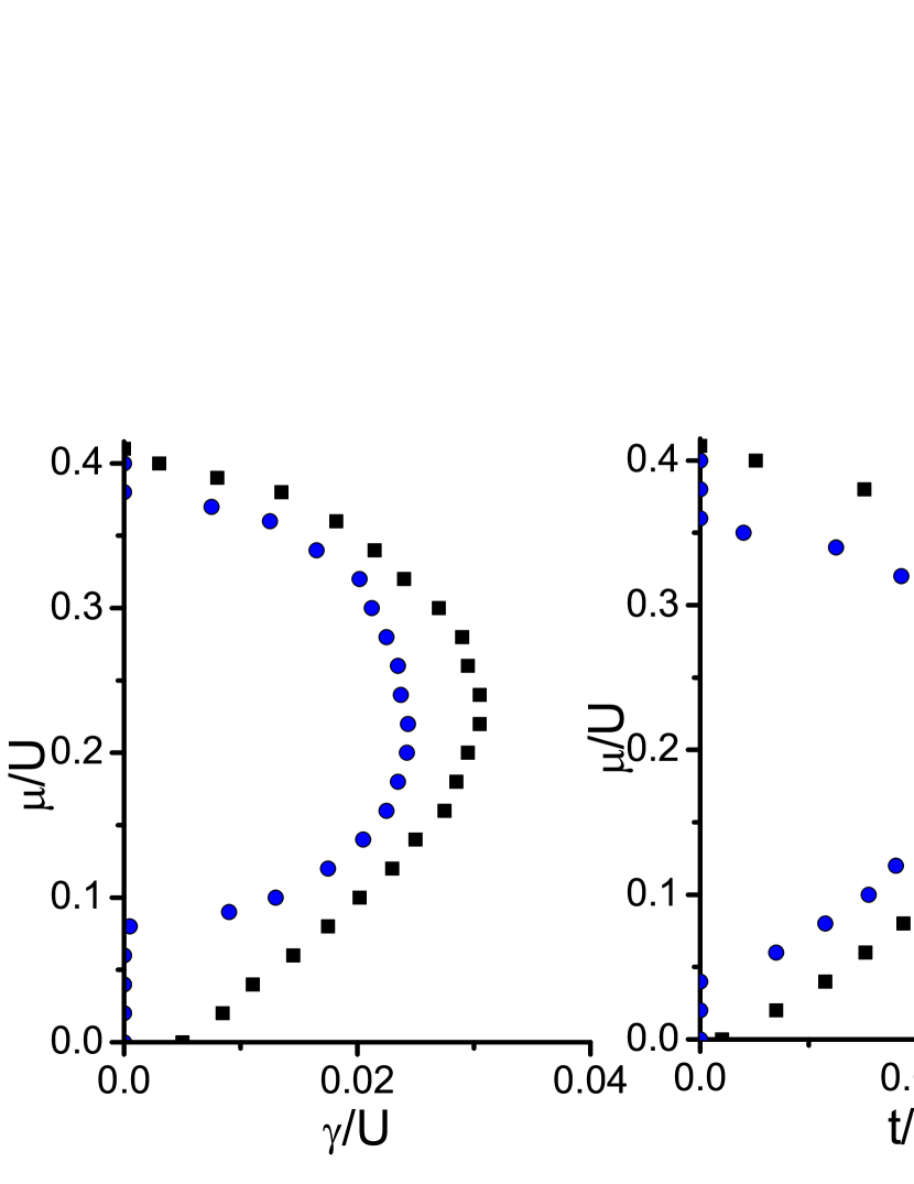
Figure 7: Left panel: The MI-SF phase boundary from mean-field theory for different representative values of $t/U=0.0$ (black squares), $t/U=0.02$ (blue circles) in the $\mu-\gamma$ plane. Right panel: The phase boundary in the $\mu-t$ plane for $\gamma/U=0$(black squares) and $\gamma/U=0.02$ (blue circles). Here we have taken $\eta=0.5$, $\delta=0.0$ and $\Omega=0.01U$.

The most striking point about the superfluid phase into which the transition takes place becomes evident on examining the values of $\Delta_{{i},a}$ for the ground state configuration in the SF phase. We find that although the amplitudes of the superfluid order parameters remain homogeneous, their phases vary with positions for finite $\gamma/t$; in other words, the superfluid ground state realized is an example of a twisted superfluid phase comment1 . We also note that the relative phases between the $x$ and the $y$ neighboring links are different leading to an anisotropic twist. To obtain an qualitative understanding of the role of spin-orbit coupling in the realization of such a twisted superfluid phase, we note that these phases contribute to the energy of the system through the terms $E_{1}$ and $E_{2}$ in Eq. 76. Taking cue from the numerical result that the magnitude of the order parameters remain constant in the ground state configuration, we now write $\Delta_{{i}a}=\Delta_{0a}\exp(i\phi_{{i}a})$. In what follows, we choose the phase of the order parameter on the ${\rm i^{th}}$ and the neighboring sites as

$$\phi_{i1} = 0,\quad\phi_{i2}=\phi_{0}$$

$$\phi_{j_{\alpha}1} = \alpha_{j_{\alpha}},\quad\phi_{j_{\alpha}2}=\beta_{j_{\alpha}},$$ (78)

where the subscript $\alpha$ takes values $x$ and $y$. Using this, one can write $E_{1}$ and $E_{2}$ in terms of the relative phases between the $x$ and $y$ neighbors

$$\frac{E_{1}}{t\Delta_{01}^{2}} = -\sum_{\langle ij\rangle}\Big{\{}[\cos(\alpha_{j_{x}})+\cos(\alpha_{j_{y}})]$$

$$+\eta\kappa^{2}[\cos(\beta_{j_{x}}-\phi_{0})+\cos(\beta_{j_{y}}-\phi_{0})]\Big{\}}$$

$$\frac{E_{2}}{t\Delta_{01}^{2}} = -\frac{\gamma\kappa}{t}\Big{[}\sum_{\langle ij_{x}\rangle}\cos(\beta_{j_{x}})+\cos(\alpha_{j_{x}}-\phi_{0})$$ (79)

$$+\sum_{\langle ij_{y}\rangle}\sin(\beta_{j_{y}})+\sin(\alpha_{j_{y}}-\phi_{0})\Big{]}$$

where $\kappa=\Delta_{02}/\Delta_{01}$.

Next, we define relative phases living on $x$ and $y$ links of the 2D square lattice as

$$\Phi_{\ell_{x}1} = \phi_{j_{x}1},\quad\Phi_{\ell_{y}1}=\phi_{j_{y}1}$$

$$\Phi_{\ell_{x}2} = \phi_{j_{x}2}-\phi_{0},\quad\Phi_{\ell_{y}2}=\phi_{j_{y}2}-\phi_{0}$$ (80)

$$\Phi_{\ell_{x}3}=\phi_{j_{x}1}-\phi_{0}.$$

In terms of these phases, Eq. 79 can be recast as

$$\frac{E_{1}}{t\Delta_{01}^{2}} = -\sum_{\ell_{x},\ell_{y}}\Big{\{}[\cos(\Phi_{\ell_{x}1})+\cos(\Phi_{\ell_{y}1})]$$

$$+\eta\kappa^{2}[\cos(\Phi_{\ell_{x}2})+\cos(\Phi_{\ell_{y}2})]\Big{\}}$$

$$\frac{E_{2}}{t\Delta_{01}^{2}} = -\frac{\gamma\kappa}{t}\sum_{\ell_{x},\ell_{y}}\Big{[}\cos(\Phi_{\ell_{x}3})-\cos(\Phi_{\ell_{x}2}-\Phi_{\ell_{x}3}+\Phi_{\ell_{x}1})$$ (81)

$$+\sin(\Phi_{\ell_{x}2}-\Phi_{\ell_{x}3}+\Phi_{\ell_{y}1})$$

$$+\sin(\Phi_{\ell_{y}2}-\Phi_{\ell_{x}2}+\Phi_{\ell_{x}3})\Big{]}$$

From Eq. 81, we clearly see that unless $\gamma/t$ is small, the minimal energy configuration correspond to non-zero but uniform values relative phases over $x$ and $y$ links. Note that the precise numerical values of these phases depend on $\kappa$ and hence requires input from numerical minimization of Eq. 76. However, once we know the value of $\kappa$, we find that the relative phases for the minimum energy are the solutions of the coupled transcendental equations $\partial(E_{1}+E_{2})/\partial\Phi_{\ell_{x(y)}1(2,3)}=0$ which yields

$$\sin(\Phi_{\ell_{x}1})-\frac{\gamma\kappa}{t}\sin(\Phi_{\ell_{x}2}-\Phi_{\ell_{x}3}+\Phi_{\ell_{x}1})=0$$

$$\sin(\Phi_{\ell_{y}1})-\frac{\gamma\kappa}{t}\cos(\Phi_{\ell_{x}2}-\Phi_{\ell_{x}3}+\Phi_{\ell_{y}1})=0$$

$$\eta\kappa^{2}\sin(\Phi_{\ell_{x}2})-\frac{\gamma\kappa}{t}\Big{\{}\sin(\Phi_{\ell_{x}2}-\Phi_{\ell_{x}3}+\Phi_{\ell_{x}1})+\cos($$

$$\Phi_{\ell_{x}2}-\Phi_{\ell_{x}3}+\Phi_{\ell_{y}1})-\cos(\Phi_{\ell_{y}2}-\Phi_{\ell_{x}2}+\Phi_{\ell_{x}3})\Big{\}}=0$$

$$\eta\kappa^{2}\sin(\Phi_{\ell_{y}2})-\frac{\gamma\kappa}{t}\sin(\Phi_{\ell_{y}2}-\Phi_{\ell_{x}2}+\Phi_{\ell_{x}3})=0$$

$$\sin(\Phi_{\ell_{x}3})+\sin(\Phi_{\ell_{x}2}-\Phi_{\ell_{x}3}+\Phi_{\ell_{x}1})+\cos(\Phi_{\ell_{x}2}$$

$$-\Phi_{\ell_{x}3}+\Phi_{\ell_{y}1})-\cos(\Phi_{\ell_{y}2}-\Phi_{\ell_{x}2}+\Phi_{\ell_{x}3})=0$$ (82)

In general, these equations need to be solved numerically and we have not found analytic solutions for them for arbitrary values of $\kappa$ and $\gamma/t$. However, in the special case $\gamma/t\gg 1$, we find that these equations admit an easy solution

$$\Phi_{\ell_{x}1} = -\Phi_{\ell_{y}1}=\pi/4,\quad\Phi_{\ell_{x}3}=\pi$$

$$\Phi_{\ell_{x}2} = -\Phi_{\ell_{y}2}=3\pi/4$$ (83)

The corresponding phase distribution of the superfluid order parameter $\phi_{{i}a}\equiv(\phi_{{i}1},\phi_{{i}2})$ is shown in the right panel of Fig. 8. For all values of $\gamma/t$ and $\kappa$, we find $\Phi_{\ell_{x}1(2)}=-\Phi_{\ell_{y}1(2)}$. Also, for $\eta<1$ (which implies $\kappa<1$), we find that $\Phi_{\ell_{x,y}2}$ have a discontinuous jump to finite value around $\gamma=0$. The occurrence of this can be easily understood a competition between second and the third set of terms ( those proportional to $\eta\kappa^{2}$ and $\gamma\kappa/t$ respectively) in Eq. 81. A plot of the relative phases on the $x$ and $y$ links is shown in the left panel of Fig. 8 as a function $\gamma/t$. We find that the relative phases take finite value for non-zero $\gamma$ and approaches those given by Eq. 83 with increasing $\gamma/t$ thus leading to the realization of a twisted superfluid ground state. We have checked that the value of the relative phases obtained from minimization of Eq. 81 agrees to those computed from minimization of Eq. 76.

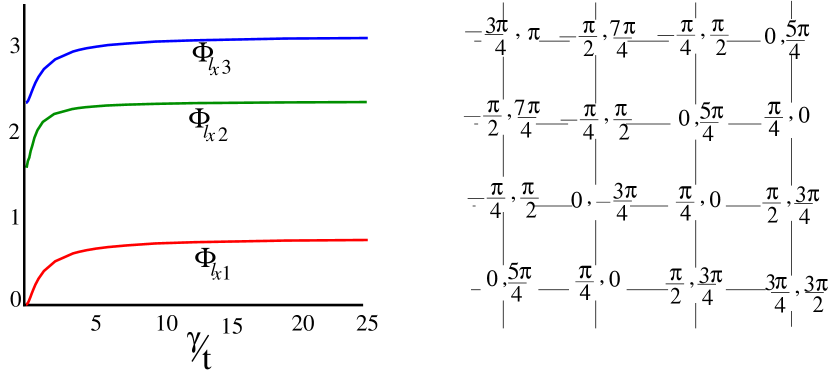
Figure 8: Left panel: Plot of the relative phases $\Phi_{\ell_{x,y}1,2,3}$ on the links of the square lattice as a function of $\gamma/t$ for $\eta=0.5$, $\Omega=0.01U$. Right panel: Distribution of the phases $\phi_{{i}a}$ for the superfluid order parameter for $\gamma/t\gg 1$.

V Collective modes

In this section, we use the critical theory developed in Sec. III.1 to obtain the collective modes in the superfluid phase near the critical point. We first consider the case $\delta=0$ for which one can obtain straightforward analytical expressions for these modes. We first consider $t=0$. We begin with the quadratic and quartic parts of the boson action in the SF phase near the critical point which are given by

$$S^{{}^{\prime}} = S^{{}^{\prime}}_{2}+S^{{}^{\prime}}_{4}$$

$$S^{{}^{\prime}}_{2} = -\int\frac{d^{2}kd\omega}{(2\pi)^{3}}\sum_{i=1,2}\xi_{i}^{\ast}\left(K_{0}\omega+K_{1}\omega^{2}\right.$$ (84)

$$\left.-v^{2}|{\bf k}|^{2}+|r_{0}|\right)\xi_{i}$$

$$S^{{}^{\prime}}_{4} = \frac{g}{2}\int d^{2}rdt\left[(|\xi_{1}|^{2}+|\xi_{2}|^{2})^{2}+\eta_{0}(|\xi_{1}|^{2}-|\xi_{2}|^{2})^{2}\right]$$

In the SF phase, both the fields condense with amplitudes $|\xi_{i0}|=\sqrt{|r_{0}|/2g}$ for $i=1,2$. To obtain the collective modes, we therefore expand the fields $\xi_{i}=\xi_{i0}+\delta\xi_{i}$, where $\delta\xi_{i}$ represents small amplitudes fluctuating fields which describes the collective modes of the condensate. Using Eq. 84, we obtain an effective quadratic action for $\delta\chi_{i}$. It turns out that for $\eta_{0}=1$, the quadratic actions for $\delta\xi_{1}$ and $\delta\xi_{2}$ reduces to block-diagonal form which can be written as

$$S^{\prime} = \int\frac{d^{2}kd\omega}{(2\pi)^{3}}\sum_{i=1,2}\Psi_{i}^{*}{\tilde{\Lambda}}\Psi_{i},$$

$${\tilde{\Lambda}} = \left(\begin{array}[]{cc}D_{0}(\omega,{\bf k})+|r_{0}|&\frac{|r_{0}|}{2}\\ \frac{|r_{0}|}{2}&D_{0}(-\omega,-{\bf k})+|r_{0}|\end{array}\right)$$ (87)

where $\Psi_{i}=\left(\delta\xi^{*}_{i},\delta\xi_{i}\right)^{T}$, and $D_{0}(\omega,{\bf k})=-(K_{1}\omega^{2}+K_{0}\omega-v^{2}|{\bf k}|^{2}+|r_{0}|)/2$. The collective modes corresponding to the field $\xi_{i}$ can then be obtained from the condition ${\rm Det}{\tilde{\Lambda}}=0$ and yields,

$$\omega_{1(2)}({\bf k}) = \sqrt{\frac{\pm\alpha_{\bf k}+\sqrt{\alpha_{\bf k}^{2}+4(A_{\bf k}^{2}-|r_{0}|^{2})K_{1}^{2}}}{2K_{1}^{2}}}$$

$$\alpha_{\bf k} = 2K_{1}A_{\bf k}+K_{0}^{2},\quad A_{\bf k}=v^{2}|{\bf k}|^{2}+|r_{0}|$$ (88)

Each of these two modes are doubly degenerate. It is easy to see from Eq. 88 that $\omega_{2}({\bf k})$ are gapped while $\omega_{1}({\bf k})$ is gapless with $\omega_{1}\sim|{\bf k}|^{2}$ at small $|{\bf k}|$ for $K_{0}\neq 0$ and $\omega_{1}=|{\bf k}|v/\sqrt{K_{1}}$ for $K_{0}=0$. The mass of the gapped mode can be read off from Eq. 88 and are given by

$$m = \sqrt{(2|r_{0}|K_{1}+K_{0}^{2})/K_{1}^{2}}$$ (89)

Note that in this case, there is one gapless and one gapped mode and each of these are doubly degenerate. This leads to two gapless modes in the SF phase which is a consequence of condensation of both $\xi_{1}$ and $\xi_{2}$ at the transition.

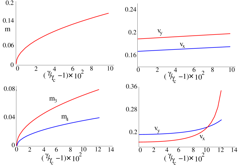
Figure 9: Left upper panel: Plot of the mass of the gapped mode for $t=0$ and $\delta=0.005U$ as a function of $(\gamma/\gamma_{c}-1)$. Upper right panel: Plot of the velocities of the gapless modes ($v_{x}$ and $v_{y}$) as a function of $(\gamma/\gamma_{c}-1)$. Lower left (right) panel: Mass of the non-condensed modes (Velocity of the gapless mode) for $t/\gamma=0.005$, $K_{0}=0$ and $\delta=0.005U$.

Next we consider the case $t/\gamma\neq 0$. In this case, we begin with the action

$$S^{{}^{\prime\prime}} = S^{{}^{\prime\prime}}_{2}+S^{{}^{\prime\prime}}_{4}$$

$$S^{{}^{\prime}}_{2} = -\int d^{2}rdt\sum_{i=1,2}\varphi_{i}^{\ast}\left(K_{0}\omega+K_{1}\omega^{2}-v^{2}|{\bf k}|^{2}+|r_{0}|\right)\varphi_{i}$$

$$S^{{}^{\prime\prime}}_{4}=\frac{g}{2}\int d^{2}rdt\left[(|\varphi_{1}|^{2}+|\varphi_{2}|^{2})^{2}+\eta^{\prime}_{0}|\varphi_{1}|^{2}|\varphi_{2}|^{2}\right].$$

To obtain the collective modes, we note that the field $\varphi_{1}$ condenses with an amplitude $|\varphi_{01}|=\sqrt{|r_{0}|/g}$. We then expand the fields $\varphi_{1}=\varphi_{01}+\delta\varphi_{1}$ and $\varphi_{2}=\delta\varphi_{2}$ and obtain the effective quadratic action for the field $\delta\varphi_{1,2}$. It turns out that these actions decouple. The effective action for $\delta\varphi_{1}$ turns out to be analogous to Eq. 87 and yields a gapless and a gapped mode with $\omega=\omega_{1(2)}({\bf k})$. The effective action for $\delta\varphi_{2}$ is given by

$$S^{{}^{\prime\prime}} = \int\frac{d^{2}kd\omega}{(2\pi)^{3}}\Psi_{2}^{{}^{\prime}*}\Lambda^{{}^{\prime\prime}}\Psi^{\prime}_{2},$$

$$\Lambda^{{}^{\prime\prime}} = \left(\begin{array}[]{cc}D_{0}(\omega,{\bf k})+(2+\eta^{\prime}_{0})|r_{0}|/2&0\\ 0&D_{0}(-\omega,-{\bf k})+(2+\eta^{\prime}_{0})|r_{0}|/2\end{array}\right)$$ (93)

where $\Psi^{\prime}_{2}=[\varphi_{2}(\omega,{\bf k}),\varphi_{2}^{\ast}(-\omega,-{\bf k})]^{T}$. The collective modes obtained using Eq. 93 are given by

$$\omega_{3(4)}({\bf k}) = \frac{-(+)K_{0}+\sqrt{K_{0}^{2}+4K_{1}(A_{\bf k}+\eta^{\prime}_{0}|r_{0}|)}}{2K_{1}}$$ (94)

The masses of these modes are given by

$$m_{3(4)} = \frac{-(+)K_{0}+\sqrt{K_{0}^{2}+4K_{1}|r_{0}|(1+\eta^{\prime}_{0})}}{2K_{1}}$$ (95)

Thus in this case, we have one gapless and three gapped mode. We note that since $K_{0}$, $K_{1}$ and $v$ can be computed from microscopic parameters of the theory, our analysis provides a way of obtaining the velocities and masses of the gapped and the gapless collective modes directly from the parameters of the microscopic Hamiltonian of the bosons.

The inclusion of finite $\delta$ changes this picture in two essential ways. First, it lifts the degeneracy between some of the modes. Second, it makes the dispersion anisotropic since in the presence of a finite $\delta$, $v_{x}$ and $v_{y}$ are not identical. A plot of the masses of the gapped and velocity of the gapless modes for a finite but small $\delta=0.005U$ is shown in Fig. 9. In accordance with the expectation, we find that the velocities of the gapless modes are different.

VI Discussion

In this work, we have studied the SI transition of two-species bosons with spin-orbit coupling. The main conclusions of our work are the following. First we have shown, via explicit calculation of the boson momentum distribution function, that the SI transition is accompanied by precursor peaks in the MI phases near the transition and that the position of these peaks can be tuned by tuning the strength of the spin-orbit coupling. We note that this feature of our theory can be directly verified experimentally by routine momentum distribution measurements Greiner1 ; spielman1 . Second, we have analyzed the MI-SF phase boundary and have shown the existence of reentrant SI transitions at fixed $t$ and $\eta$ with variation of $\gamma$. This feature can also be detected experimentally by momentum distribution measurements. Third, we have shown that for $t/\gamma=0$, the SI transition is unconventional in the sense that it is accompanied by emergence of a gapless mode in the critical region. Fourth, we have computed the collective modes in the SF phase near the transition. We have presented analytical formulae for the gapless and the gapped mode and have provided explicit expression for their masses and velocities in terms of microscopic parameters of theory. These predictions can be verified by routine spectroscopy measurements on these systems esslinger1 . Finally, our mean-field study has revealed the presence of a twisted superfluid ground state in these systems with an anisotropic twist angle whose magnitude depend on $\gamma/t$.

KS thanks DST for support through grant SR/S2/CMP-001/2009.

References

- (1) M. Greiner, O. Mandel, T. Esslinger, T. W. HaÈnsch, and I. Bloch, Nature 415, 39 (2002);
- (2) C. Orzel, A. K. Tuchman, M. L. Fenselau, M. Yasuda, and M. A. Kasevich, Science 291, 2386 (2001).
- (3) M. P. A. Fisher, P. W. Weichman, G. Grinstein, and D. S. Fisher, Phys. Rev. B 40, 546 (1989).
- (4) S. Sachdev, Quantum Phase transitions, Cambridge University Press, (1999).
- (5) D. Jaksch, C. Bruder, J. I. Cirac, C. W. Gardiner, and P. Zoller , Phys. Rev. Lett. 81, 3108 (1998).
- (6) K. Seshadri, H. R. Krishnamurthy, R. Pandit, and T. V. Ramakrishnan, Europhys. Lett. 22, 257 (1993);
- (7) M. Krauth and N. Trivedi, Europhys. Lett.14, 627 (1991)
- (8) B. Capogrosso-Sansone, N. N. Prokofev, and B.V. Svistunov, Phys. Rev. B 75, 134302 (2007).
- (9) C. Trefzer and K. Sengupta, Phys. Rev. Lett. 106, 095702 (2011); A. Dutta, C. Trefzger, and K. Sengupta, arXiv:1111. (unpublihsed).
- (10) J. Freericks, H. R. Krishnamurthy, Y. Kato, N. Kawashima, and N. Trivedi, Phys. Rev. A79, 053631 (2009).
- (11) K. Sengupta and N. Dupuis, Phys. Rev. A71, 033629 (2005).
- (12) I. B. Spielman, W. D. Phillips, and J. V. Porto, Phys. Rev. Lett. 98, 080404 (2007).
- (13) D. Jaksch and P. Zoller, New J. Phys. 5, 56 (2003); E. Mueller, Phys. Rev. A 70, 041603(R) (2004); K. Osterloh, M. Baig, L. Santos, P. Zoller, and M. Lewenstein, Phys. Rev. Lett. 95, 010403 (2005); N. Goldman, A. Kubasiak, P. Gaspard, and M. Lewenstein, Phys. Rev. A79, 023624 (2009); I. B. Spielman, Phys. Rev. A 79, 063613 (2009).
- (14) Y-J. Lin, R. L. Compton, A. R. Perry, W.D. Phillips, J.V. Porto, and I. B. Spielman, Phys. Rev. Lett. 102, 130401 (2009).
- (15) Y.-J. Lin,R. L. Compton, K. Jime´nez-Garcı´a, J. V. Porto, and I. B. Spielman, Nature 462, 628-632 (2009).
- (16) S. Sinha and K. Sengupta, EuroPhys. Lett. 93 30005 (2011); S. Powel, R. Barnett, R. Sensarma, S. D. Sarma, Phys. Rev. Lett. 104 255303 (2010); K. Saha, K. Sengupta, and K. Ray, Phys. Rev. B82 205126 (2010)
- (17) T. Grass, K. Saha, K. Sengupta, and M. Lewenstein, Phys. Rev. A84, 053632 (2011).
- (18) R. Sensarma, K. Sengupta, and S. Dassarma, Phys. Rev. B84, 081101 (2011).
- (19) X-L Qi and S.C. Zhang, Rev. Mod. Phys. 83 1057 (2011).
- (20) G. Juzeliunas et al., Phys. Rev. A 77, 011802(R) (2008); T. D. Stanescu, B. Anderson and V. Galitski, Phys. Rev. A 78, 023616 (2008); X.-J. Liu, X. Liu, L. C. Kewk, and C. H. Oh, Phys. Rev. Lett. 98, 026602 (2007); J. D. Sau et al., Phys. Rev. B 83, 140510(R) (2011); D. L. Campbell, G. Juzeliunas, and I. B. Spielman, arXiv:1102.3945 (unpublished).
- (21) Y. J. Lin et al. Nature 471, 83 (2011).
- (22) C. Wu and I. Mondragon-Shem arXiv:0809.3532v1(unpublished); C. Wu , I. Mondragon Shem, and X. F. Zhou, Chin. Phys. Lett. 28, 097102 (2011).
- (23) S. K. Yip, Phys. Rev. A 83, 043616 (2011).
- (24) J. Larson, J. P. Martikainen, A. Collin, and E. Sjoqvist, arXiv:1001.2527 (unpublished).
- (25) M. Merkl et al., Phys. Rev. Lett. 104, 073603 (2010).
- (26) C. Wang, C. Gao, C.-M. Jian and H. Zhai, Phys. Rev. Lett. 105, 160403 (2010).
- (27) Y. Li, X. Zhou, and C. Wu, arXiv:1205.2162 (unpublished); X-F Zhow, J, Zhou, and C. Wu, Phys. Rev. A84, 063624 (2011).
- (28) Y. Zhang, L. Mao and C. Zhang, arXiv:1102.4045 (unpublished).
- (29) S. Sinha, R. Nath, and L. Santos Phys. Rev. Lett. 107, 270401 (2011).
- (30) J. P. Vyasankere and V. B. Shenoy, arXiv:1201.5332 (unpublished).
- (31) J. Radic, A. di Colo, K. Sun, and V. Galitski, arXiv:1205.2110 (unpublised).
- (32) W.S. Cole, S. Zhang, A. Paramekanti, and N. Trivedi, arXiv: 1205.2319 (unpublished).
- (33) Z. Cai, X. Zhou, and C. Wu, arXiv:1205.3116 (unpublised).
- (34) A. Issacson, M-C Cha, K. Sengupta, and S. M. Girvin, Phys. Rev. B72, 184507 (2005).
- (35) E. Altman, W. Hofstetter, E. Demler, and M. D. Lukin, New J. Phys. 5, 113 (2003); L-M. Duan, E. Demler, and M. D. Lukin, Phys. Rev. Lett. 91, 090402 (2003); A. B. Kuklov and B. V. Svistunov, Phys. Rev. Lett. 90, 100401 (2003); A. Kuklov, N. Prokof ev, and B. Svistunov, ibid. 92, 050402 (2004).
- (36) F. D. M. Haldane, Phys. Rev. Lett. 61, 2015 (1988).
- (37) L. Balents, L. Bartosch, A. Burkov, S. Sachdev, and K. Sengupta Phys. Rev. B71, 144508 (2005).
- (38) Such a twisted superfluid phase have been reported in other systems; for example see, P. Soltan-Panahi, D. Luhmann, J. Struck, P. Windpassinger, and K. Sengstock, Nat. Phys. 8, 71 (2012).
- (39) C. Schori, T. Stoferle, H. Moritz, M. Kohl, and T. Esslinger, Phys. Rev. Lett. 93, 240402 (2004); D. Greif, L. Tarruell, T. Uehlinger, R. Jordens, and T. Esslinger, Phys. Rev. Lett. 106, 145302 (2011).