Maximally Star-Forming Galactic Disks II. Vertically-Resolved Hydrodynamic Simulations of Starburst Regulation

Abstract

We explore the self-regulation of star formation using a large suite of high resolution hydrodynamic simulations, focusing on molecule-dominated regions (galactic centers and [U]LIRGS) where feedback from star formation drives highly supersonic turbulence. In equilibrium the total midplane pressure, dominated by turbulence, must balance the vertical weight of the ISM. Under self-regulation, the momentum flux injected by feedback evolves until it matches the vertical weight. We test this flux balance in simulations spanning a wide range of parameters, including surface density $\Sigma$, momentum injected per stellar mass formed ($p_{*}/m_{*}$), and angular velocity. The simulations are two dimensional radial-vertical slices, and include both self-gravity and an external potential that helps to confine gas to the disk midplane. After the simulations reach a steady state in all relevant quantities, including the star formation rate $\Sigma_{\rm SFR}$, there is remarkably good agreement between the vertical weight, the turbulent pressure, and the momentum injection rate from supernovae. Gas velocity dispersions and disk thicknesses increase with $p_{*}/m_{*}$. The efficiency of star formation per free-fall time at the mid-plane density, $\epsilon_{\rm ff}(n_{\rm 0})$, is insensitive to the local conditions and to the star formation prescription in very dense gas. We measure $\epsilon_{\rm ff}(n_{\rm 0})$$\sim$0.004-0.01, consistent with low and approximately constant efficiencies inferred from observations. For $\Sigma$$\in$(100–1000) M_⊙ pc^-2, we find $\Sigma_{\rm SFR}$$\in$(0.1–4) ${\rm M}_{\odot}\,{\rm kpc}^{-2}\,{\rm yr}^{-1}$, generally following a $\Sigma_{\rm SFR}$$\propto$ $\Sigma$² relationship. The measured relationships agree very well with vertical equilibrium and with turbulent energy replenishment by feedback within a vertical crossing time. These results, along with the observed $\Sigma$–$\Sigma_{\rm SFR}$ relation in high density environments, provide strong evidence for the self-regulation of star formation.

1. Introduction

1.1. Star Formation on Galactic Scales

Observations reveal that stars form in the molecular component of the interstellar medium (ISM). Therefore, the dynamics of molecular gas must affect the star formation process. On galactic scales, gravity concentrates gas into clouds in which stars eventually form. The resulting feedback from stellar winds, ionizing and non-ionizing radiation, and supernovae (SN) (either local or nearby in the disk) redisperses this dense gas. The formation, destruction, and the dynamical state of star forming clouds depend strongly on the local conditions of the ISM. In (ultra) luminous infrared galaxies ([U]LIRGs) and the centers of galaxies, molecular gas pervades much of the ISM, including regions not actively forming stars. Gas in such environments has higher mean volume and surface density compared to the gas found in giant molecular clouds (GMCs, Solomon & Vanden Bout, 2005) in lower-density regions of galaxies. Near-future ALMA observations will resolve high density tracers, and thereby reveal the detailed structure and kinematics of gas in starbursts. Understanding how small-scale feedback associated with star-formation acts in concert with larger scale processes in starbursts (as well as mid– and outer– disks) is crucial for developing any successful theory of galactic star formation.

Stellar feedback plays a key role in regulating the thermal balance and morphological structure of the ISM (McKee & Ostriker, 1977; Norman & Ikeuchi, 1989). Feedback is also believed to be the primary mechanism driving turbulence (e.g. Norman & Ferrara, 1996). Since turbulence is observed on all scales larger than the size of the densest prestellar cores, it is now understood to be an essential component controlling the dynamics and regulating star formation in the ISM (see Mac Low & Klessen, 2004; McKee & Ostriker, 2007, and references therein). The vertical scale height of the galactic disk depends on the balance between gaseous, stellar, and dark matter potentials that concentrate gas, and the pressures (thermal, turbulent, magnetic, cosmic ray, and radiation) that oppose gravity and limit runaway collapse (e.g. Boulares & Cox, 1990).

Over sufficiently large scales, the star formation rate surface density, $\Sigma_{\rm SFR}$, is observed to correlate well with the gas surface density, $\Sigma$ (Schmidt, 1959; Kennicutt, 1989, 1998). This correlation appears to take on various forms in different regions within disk galaxies. In the outer-disk regions containing little molecular gas, there is no universal power-law index describing the $\Sigma_{\rm SFR}$$-$$\Sigma$ relationship (Bigiel et al., 2010). Instead, $\Sigma_{\rm SFR}$ depends on both $\Sigma$ and the stellar density (Blitz & Rosolowsky, 2004, 2006); this is presumably because stellar rather than gas vertical gravity dominates in outer disks (see below). At smaller radii, by mass the ISM is dominated by molecular gas, for which two different star formation laws appear to take hold. In mid-disk regions where most of the volume is filled with atomic gas and molecules are confined in isolated GMCs (with a limited range of properties – Sheth et al. (2008); Bolatto et al. (2008)), there is a strong, approximately linear correlation between the star formation rate and molecular mass, $\Sigma_{\rm SFR}$ $\propto$ $\Sigma_{\rm mol}$ (Wong & Blitz, 2002; Bigiel et al., 2008; Schruba et al., 2011). Towards the central regions and in starbursts where the ISM is almost completely molecular (Solomon & Vanden Bout, 2005), there appears to be a steeper $\Sigma_{\rm SFR}$– $\Sigma_{\rm mol}$ relationship (Kennicutt, 1998; Genzel et al., 2010; Daddi et al., 2010; Narayanan et al., 2012).

The variations in $\Sigma$–$\Sigma_{\rm SFR}$ correlations in different galactic regions presumably owe to the differences in the characteristics of the ISM. Gas properties such as the temperatures, densities, and velocities are found to vary between starbursts and more quiescent environments. In the Galactic center, molecular gas is much more prevalent (e.g. Bally et al., 1987, 1988), and $\Sigma_{\rm SFR}$ is measured to be $\sim$1.5 dex higher than in the mid- to outer- disk (Yusef-Zadeh et al., 2009). Observed linewidths from the dense, molecular gas in the Galactic Center are measured to reach  $\buildrel>\over{\sim}$ 10 km s^-1 (Oka et al., 1998, 2001; Shetty et al., 2012), and as high as  $\buildrel>\over{\sim}$ 100 km s^-1 in starbursts (Solomon et al., 1997; Downes & Solomon, 1998; Genzel et al., 2011). Turbulent velocities in GMCs are significantly lower, ranging from 1 – 6 km s^-1 (e.g. Larson, 1981; Solomon et al., 1987). However, present observations of (U)LIRGs do not have sufficient resolution to distinguish between perturbed motions (such as large-scale streaming) on scales $\ {\raise-2.15277pt\hbox{$\buildrel>\over{\sim}$}}\ H$, the disk thickness, and more localized turbulence (i.e. velocity dispersions on $\sim$10 pc scales, similar to GMCs).

Global numerical simulations of disk galaxies have shown that the structures formed by self-gravity (e.g. Shetty & Ostriker, 2006; Dobbs & Pringle, 2009; Tasker & Tan, 2009; Tasker, 2011) or by cloud collisions (e.g. Dobbs, 2008; Tasker & Tan, 2009) can generally reproduce observed morphological features of the ISM, such as filamentary substructure, cloud masses, sizes, and basic kinematic properties. Additionally, large scale simulations have suggested that gravitational instability naturally results in power-law relationships between $\Sigma_{\rm SFR}$ and $\Sigma$ if the Toomre $Q$ and velocity dispersion are uniform (e.g. Li et al., 2005, 2006; Shetty & Ostriker, 2008). Simulations with feedback have produced a range in the exponent and coefficient of the $\Sigma_{\rm SFR}$-$\Sigma$ relationship, depending on the specific feedback prescription (e.g Tasker & Bryan, 2006, 2008; Robertson & Kravtsov, 2008; Shetty & Ostriker, 2008; Koyama & Ostriker, 2009a; Dobbs et al., 2011; Hopkins et al., 2011). Shetty & Ostriker (2008) pointed out that the relationship between $\Sigma_{\rm SFR}$ and $\Sigma$ in general should depend on the thickness of the gas disk, and therefore on the gas velocity dispersion and on the stellar potential if it dominates (see below).

Variations in feedback parameters, such as the injected momenta, energies, and rates, combined with other processes such as rotation, vertical motions due to an external potential, shear, and large-scale gravitational instability in the shearing, rotating flow, are likely to contribute to the observed differences in velocity dispersions between starbursts and more quiescent regions. Ostriker & Shetty (2011) and Kim et al. (2011) (hereafter KKO11) argue that the velocity dispersion on scales comparable to the neutral gas disk’s thickness will be relatively constant if turbulence is driven by feedback, because the driving rate and dissipation rate both scale inversely with the vertical crossing time (or gravitational free-fall time) of the ISM. Simulations of the ISM in mid– and outer– disk environments have shown that velocity dispersions are in fact not strongly sensitive to the feedback parameters (e.g. Dib et al., 2006; Shetty & Ostriker, 2008; Joung et al., 2009, KKO11). Such simulations allow for a detailed assessment of the relationships between the relevant physical quantities, and provide a direct avenue for testing analytical theories of star formation.

1.2. Theory of Star Formation Self-Regulation

A theory for the self-regulation of star formation on galactic scales has recently been formulated by Ostriker et al. (2010) (hereafter OML10) and Ostriker & Shetty (2011) (hereafter Paper I). KKO11 conducted numerical models of multi-phase gaseous disks in the regime where diffuse atomic gas dominates ($\Sigma$  $\buildrel<\over{\sim}$ 20 M_⊙ pc^-2), verifying the assumptions and predicted features of the self-regulated thermal/dynamical equilibrium theory. In the present work, we shall instead focus on numerical simulations of the molecule-dominated starburst regime. To provide an overall context and distinguish between the various regimes, we briefly review the concepts and analysis of the self-regulation model.

For dynamical equilibrium to be satisfied, the total pressure at the midplane must balance the gravitational weight of the overlying diffuse-ISM gas, $P_{\rm tot}=W\equiv(1/2)\Sigma_{\rm diff}\langle g_{z}\rangle$. In different regimes, this pressure may be dominated by different terms (thermal, turbulent, or radiation), but each pressure term individually responds to the star formation rate. Where there is a substantial amount of atomic gas heated by stellar UV, balance of heating and cooling leads to an equilibrium thermal pressure $P_{\rm th}\propto J_{\rm UV}\propto\Sigma_{\rm SFR}$ (OML10, KKO11). Similarly, balancing turbulent driving associated with expanding radiative SN remnants (or other massive-star momentum sources) with dissipation on a vertical crossing time leads to an equilibrium turbulent pressure $P_{\rm turb}\propto\Sigma_{\rm SFR}$ (Paper I, KKO11). In extremely high $\Sigma$ regions, trapped reprocessed starlight provides a radiation pressure $P_{\rm rad}\propto\Sigma\Sigma_{\rm SFR}$ that begins to compete with the turbulent pressure (Thompson et al., 2005, Paper I). Putting these individual terms together, $P_{\rm tot}=P_{\rm th}+P_{\rm turb}+P_{\rm rad}\propto\Sigma_{\rm SFR}$. Thus, under self-regulation the combined constraints of thermal, turbulent, radiative, and dynamical equilibrium imply that the star formation rate will naturally evolve to a level imposed by the vertical gravitational field, $\Sigma_{\rm SFR}\propto W$.

In mid- and outer-disk regions (generally where $\Sigma$  $\buildrel<\over{\sim}$  100 M_⊙ pc^-2), the warm ($T\sim 10^{4}$ K) ISM is space-filling and GMCs appear to be self-gravitating structures that do not participate in the general vertical equilibrium. For this regime, OML10 show that the thermal/dynamical equilibrium theory is in good agreement with observations, with $\Sigma_{\rm SFR}$ depending on both $\Sigma$ and the stellar density $\rho_{*}$ of the disk (see also KKO11). For outer disks, diffuse HI dominates and $\Sigma_{\rm SFR}\propto\Sigma\sqrt{\rho_{*}}$ because the weight of the diffuse ISM is $W\propto\Sigma\sqrt{\rho_{*}}$ in this regime. For mid-disks, gas is concentrated in gravitationally-bound clouds (observed as GMCs) which have relatively uniform column density, star formation efficiency, and other properties (probably as a result of internal feedback), such that $\Sigma_{\rm SFR}\propto\Sigma$.

In very dense regions where $\Sigma$ $\buildrel>\over{\sim}$ 100 M_⊙ pc^-2, such as the Galactic center and ULIRGs, UV heating is not expected to play a strong role, and molecular gas is pervasive rather than concentrated in effectively isolated GMCs. The transition to the “diffuse molecular” starburst regime occurs where the pressure of the ISM as a whole exceeds the pressure of isolated, bound GMCs as found in the outer disk. For bound or virialized GMCs with surface density $\Sigma_{\rm GMC}\equiv M/(\pi R^{2})$ that have a gravitational-to-kinetic energy ratio of 1 to 2, the internal pressure is $(0.5-1)G\Sigma_{\rm GMC}^{2}$. The ISM as a whole must have midplane pressure $(\pi/2)G\Sigma^{2}$ if equilibrium holds and gas dominates the gravity (see Equation [10] below); from Paper I, this pressure is primarily turbulent, driven by star formation feedback. The transition to the regime where molecular clouds lose their identity (and may be destroyed by externally-driven turbulence rather than internal feedback) therefore occurs when $\Sigma\gtrsim(0.5-0.8)\Sigma_{\rm GMC}\sim 50-100$ M_⊙ pc^-2.

In the starburst regime, the theory of Paper I suggests that SN play a key role in controlling the overall star formation rates because they dominate the momentum injection rate to the ISM. Paper I presented the analytical theory, compared the star formation rates to observations compiled in Genzel et al. (2010), and provided initial results from numerical models of SN-driven turbulent feedback in a cold ISM. According to the theory of Paper I, $\Sigma_{\rm SFR}\propto\Sigma^{2}$ is expected for most starbursts (see Equation 13 below). Here, we extend Paper I to test the predictions from self-regulation over a wide range of galaxy and feedback parameters, using time-dependent numerical simulations.

1.3. Simulations of Self-Regulation Due to Feedback in Starbursting Environments

In this work, we model the evolution of a molecular dominated ISM using radial-vertical simulations, including a treatment for gas motion in the azimuthal direction. Using a large suite of hydrodynamic models, we focus on the role of SN driven feedback in the starburst regime, including its relationship to other disk characteristics such as the overall star formation rate, disk thickness, and midplane density. A key feature of these simulations is that the vertical dimension is well resolved, which is important for accurately capturing the effect of turbulence on disk thickness, as pointed out by Shetty & Ostriker (2008). We test the sensitivity of the results to the assumed input parameters, such as the efficiency of star formation in dense gas, and the momentum injected per unit stellar mass. Our analysis aims to understand the role of feedback-induced turbulence on the self-regulation of star formation in high (surface) density regions, where $\Sigma$ $\buildrel>\over{\sim}$ 100 M_⊙ pc^-2, representative of the ISM in (U)LIRGs and galactic centers.

This paper is organized as follows. The next section describes the relevant equations and our numerical methods. Section 3 presents our model results, as well as a comparison between the simulations and the predictions from self-regulation theory. After a discussion we summarize our work in Section 4.

2. Numerical Methods

2.1. Basic Equations and Local Disk Model

To model the evolution of the ISM in dense molecular disks, we solve the time-dependent hydrodynamic equations, including self-gravity. The relevant equations are:

$$\frac{\partial\rho}{\partial t}+\nabla\cdot(\rho{\bf v}) = 0$$ (1)

$$\frac{\partial{\bf v}}{\partial t}+{\bf v}\cdot\nabla{\bf v} = -\frac{1}{\rho}\nabla P-2{\bf\Omega}\times{\bf v}-\nabla\Phi_{g}+{\bf g_{ext}}$$ (2)

$$\nabla^{2}\Phi_{g} = 4\pi G\rho$$ (3)

where $\rho$, ${\bf v}$, $P$, and ${\bf\Omega}$ are the volume density, velocity, pressure, and angular velocity of the rotating frame, respectively, and $G$ is the gravitational constant. Since gas cools efficiently in high density molecular regions, we employ an isothermal equation of state, with constant sound speed $c_{s}=(P/\rho)^{1/2}$. We implement a static stellar gravitational field ${\bf g_{ext}}=-\Omega^{2}z\hat{z}$ (assumed to arise from a spherical bulge), which helps to concentrate gas to the midplane. The bulge potential is also responsible for the overall rotation of the gas with angular velocity $\Omega$. The time-varying self-gravitational potential due to the gas is $\Phi_{g}$.

The domain of our simulations is two-dimensional (2D), consisting of a radial and vertical (${\bf\hat{R}},\,{\bf\hat{z}}$) cross-section of a galactic disk, with extents $L_{\rm R}$ and $L_{\rm z}$, respectively. Though the 2D simulations only treat $x=R-R_{0}$ and $z$ as independent variables, velocities in all three directions (including $\hat{\phi}$) are included. We also include Coriolis forces, with ${\bf\Omega}=\Omega\hat{z}$ constant (i.e. solid body rotation, for a constant-density bulge). We do not consider shear, as our focus is on galactic central regions, where the rotation curve is still rising. When $d\Omega/dR=0$, the tidal potential term in the rotating frame is zero and does not enter the momentum equation (this tidal term is nonzero in outer-disk regions where rotation is strongly sheared – see the right-hand side of Equation 15 of KKO11).

Additionally, in our calculation of star formation rates, we implicitly consider the extent in the azimuthal direction $L_{\rm\phi}$ (see Section 3.3). To model a local patch of the disk cross-section, we adopt periodic boundary conditions in ${\bf\hat{R}}$. In order to maintain a constant value of $\Sigma$ throughout the simulation, we also adopt periodic boundary conditions in ${\bf\hat{z}}$. As we describe in Section 3.2, we ensure that $L_{\rm z}$ is sufficiently large in order to follow the complete evolution of the supernova shells, such that the ISM scale height and star formation rate are converged. Simulating 2D (${\bf\hat{R}},\,{\bf\hat{z}}$) slices allows us to perform calculations with very high (sub-pc) spatial resolution, as well as to explore a wide range in parameter space (which may be used as a basis for future three dimensional [3D] simulations; initial tests show that similar results hold for 3D models).

We numerically integrate the hydrodynamic Equations (1) - (3) using the Athena code (Stone et al., 2008). Athena solves the partial differential equations using a single-step, directionally unsplit Godunov method in multiple dimensions (Stone & Gardiner, 2009). We adopt piecewise-linear reconstruction and the HLLC Riemann solver. To solve the time-varying self-gravitational potential $\Phi_{g}$, we employ a Fourier transform method with vacuum vertical boundary conditions and periodic horizontal boundary conditions, as described in Koyama & Ostriker (2009b). We explore a range in $L_{\rm R}$ and $L_{\rm z}$, as well as the number of zones $N_{\rm R}$ and $N_{\rm z}$, in order to ensure that the results are not sensitive to the domain extent and that the features are well resolved numerically, as we discuss in Section 3.2.

2.2. Feedback Prescription and Model Parameters

Equations (1) - (3) only describe the basic hydrodynamics, rotation, gas self-gravity, and the vertical potential. Our simulations also include an idealized model of momentum feedback produced by supernovae, which drives turbulence and disperses dense regions. This feedback mechanism increases the total pressure, and limits collapse of the gaseous disk to only a small fraction of the densest material.

Our method to identify regions that could form stars, and to apply momentum feedback that these stars would produce, is similar to that described in Shetty & Ostriker (2008). Here, we provide an overview of this algorithm, and refer the reader to Shetty & Ostriker (2008) and KKO11 for a more detailed description.

We employ a statistical approach to determine host locations for the feedback events, and how much star formation is tallied (we do not remove gas from the domain). Star formation can occur in a fraction of the regions where the number densities are greater than some chosen threshold density $n_{\rm th}$. Thus, at every time-step each grid zone with $n\geq$ $n_{\rm th}$ is identified. Next, the number of massive stars (that can produce feedback) in zones with $n\geq$ $n_{\rm th}$ is determined through a probability defined by two other user-chosen parameters, the “free-fall efficiency” (conversion of gas mass to stars per free-fall time), $\epsilon_{\rm ff}(n_{\rm th})$, and the total mass in all stars formed per high mass star, $m_{*}$. We then apply feedback instantaneously, centered on those zones where high mass stars are determined to form (i.e. we omit time delays and spatial offsets in feedback, which more realistic models would take into account). The probability of a feedback event centered on a zone with $n\geq$ $n_{\rm th}$ in a given time-step $\Delta t$ is thus

$$P=\frac{\Delta t\,\epsilon_{\rm ff}(n_{\rm th})\,M_{\rm cl}}{t_{\rm ff}\,(n_{\rm th})\,m_{*}},$$ (4)

where $M_{\rm cl}$ is the mass of gas contained in the dense cloud in which the event originates, and the free fall time is $t_{\rm ff}(n_{\rm th})$= $[3\pi/(32G\mu m_{p}n_{\rm th})]^{1/2}$; here $\mu$ is the mean molecular weight and $m_{p}$ is the proton mass. For each massive star formed in a given time step, the total mass in stars formed is augmented by $m_{*}$ (Equation 21 of KKO11).

After a zone is determined to host a supernova, a circular region with chosen radius $R_{\rm sh}$ is delineated. The density inside this region is reset to a uniform value (conserving total mass), and velocities pointing away from the center are set such that the mean (spherical) momentum injected per event is equal to $p_{*}$ (see Equation 23 of KKO11).

Table 1Symbols Employed

Symbol	Definition
Simulation Parameters
$\epsilon_{\rm ff}(n_{\rm th})$	free-fall efficiency at the threshold density
$L_{\rm R}$	physical extent in radial dimension
$L_{\rm z}$	physical extent in vertical dimension
$m_{*}$	total mass of stars per feedback event
$N_{\rm R}$	number of zones in radial dimension
$N_{\rm z}$	number of zones in vertical dimension
$n_{\rm th}$	threshold number density for feedback to occur
$\Omega$	angular velocity
$p_{*}$	injected momentum per feedback event
$R_{\rm sh}$	radius of feedback event
$\Sigma$	gas surface density
$t_{\rm orb}$	orbital time
Measured Quantities
$\epsilon_{\rm ff}(n_{\rm 0})$	free-fall efficiency at midplane density
$f_{p}$	turbulent dissipation parameter
$H$	gas disk thickness
$n_{0}$	gas number density at midplane
$P_{\rm drive}$	vertical momentum injection rate per unit area
$P_{\rm turb}$	midplane turbulent pressure
$\Sigma_{\rm SFR}$	star formation rate
$\sigma_{v}$	vertical velocity dispersion
$v_{z}$	vertical velocity
$W$	vertical weight of the gas layer
$\chi$	contribution of bulge to vertical gravity, relative to gas self-gravity

In summary, there are five user-defined parameters required to identify and implement feedback: $n_{\rm th}$, $\epsilon_{\rm ff}(n_{\rm th})$, $R_{\rm sh}$, $p_{*}$, and $m_{*}$. We adopt $m_{*}$= 100 M_⊙, which is derived from a Kroupa (2001) IMF assuming supernovae result from stars with mass $\geq$ 8 M_⊙. The chosen value of $R_{\rm sh}$ also sets the effective azimuthal thickness $L_{\rm\phi}$= 2$R_{\rm sh}$, which is used in setting $M_{\rm cl}$. The remaining three parameters, along with $\Sigma$, $\Omega$, $c_{s}$, $L_{\rm R}$, $L_{\rm z}$, and the resolution $N_{\rm R}$$\times$$N_{\rm z}$ complete the set of inputs for each numerical simulation. Table 1 lists the symbols and the corresponding description of the relevant model parameters and measured quantities we refer to throughout this paper.

Our initial vertical density profile decreases as a Gaussian away from the midplane, such that the surface density is $\Sigma$. We also include a sinusoidal perturbation along $R$, to seed gravitational instability. We have verified that our particular choice of initial conditions does not affect the later evolution in any way. As we demonstrate in the next section, by approximately one orbital time $t_{\rm orb}$= 2$\pi/\Omega$, the dynamic disk settles into a statistical steady state, such that the downward motions due to the vertical potential are countered by the upward motions due to feedback occurring near the midplane.

2.3. Missing Physics

The hydrodynamic models we consider are highly idealized, while in the real ISM a number of additional physical processes may play a role. Cosmic rays, magnetic fields, and thermal radiation can contribute pressure, and can in principle affect self-regulation of star formation. The first two are, however, likely to be less important than the turbulent pressure if cosmic ray and magnetic scale heights are large compared to that of the neutral disk, and the last is likely important only if the gas surface density is extremely high (see Paper I). The analytical model for self-regulated star formation in Paper I allows for feedback processes in addition to the turbulent driving considered here, and it will be interesting to explore these effects quantitatively in future simulations.

As our simulations represent radial-vertical slices rather than full three-dimensional regions, we cannot study the detailed morphological structure of the ISM, such as filaments and the shapes of dense clouds. Three-dimensional simulations would be necessary to characterize the masses of clouds, and to make comparisons to structures as identified in position-position-velocity molecular-line data cubes (e.g. Pichardo et al., 2000; Ostriker et al., 2001; Gammie et al., 2003; Shetty et al., 2010). Because the interior of vertically-expanding shells can be “filled” by gas moving horizontally from other azimuthal locations, the morphology in our present simulations appears more “open” than it would in a fully three dimensional model. We note, however, that three-dimensional simulations of self-regulated star formation in outer disks analogous to the radial-vertical models of KKO11 give star formation rates that are quite consistent with those obtained using radial-vertical simulations.

Because the primary focus of this work is on star formation in the molecule-dominated turbulent ISM, we have adopted the same (highly idealized) assumption of an isothermal medium that has been so fruitful in many of the first numerical studies of turbulent molecular clouds (see reviews by Mac Low & Klessen 2004 and McKee & Ostriker 2007). In reality, the ISM has much more complex thermal and chemical structure, and a number of recent numerical studies have taken these into consideration. In particular, three-dimensional simulations including detailed heating and cooling for ISM models with thermal supernova energy injection have recently been conducted by de Avillez & Breitschwerdt (2004); Joung et al. (2009); Hill et al. (2012), among others. Although most simulations including a hot ISM have focused on conditions similar to the Solar neighborhood, Joung et al. (2009) included a case with very high supernova rate, as would be expected for star formation rate $\sim 1$ ${\rm M}_{\odot}\,{\rm kpc}^{-2}\,{\rm yr}^{-1}$, similar to the starburst regime we consider here. These recent multiphase simulations have not included self-gravity, however, and thus the supernovae rate is imposed as an input parameter rather than being modulated by the mass of gravitationally-collapsing gas. It will be quite interesting to include self-gravity and a feedback implementation together with multiphase heating and cooling to model self-regulated star formation more realistically. In particular, by comparison with simulations that model supernovae by injecting thermal energy, it will be possible to assess the simple momentum injection model we adopt here to represent turbulent driving in the neutral ISM by radiative supernova remnants.

3. Results

3.1. Overview of Simulations

Table 2Input Parameters of Hydrodynamic Models

(1)	(2)	(3)	(4)	(5)	(6)	(7)	(8)
Model	$\Sigma$	$\epsilon_{\rm ff}(n_{\rm th})$	$p_{*}$	$\Omega$	$t_{\rm orb}$	$L_{R}$	$L_{z}$
	(M⊙ pc-2)		(M⊙ km s-1)	(Myr-1)	(Myr)	(pc)	(pc)
Series S	(variation in $\Sigma$)
S100	100	0.005	$3\times 10^{5}$	0.1	62.8	120	240
S200	200	0.005	3$\times 10^{5}$	0.2	31.4	60	120
S400	400	0.005	3$\times 10^{5}$	0.4	15.7	30	60
S800	800	0.005	3$\times 10^{5}$	0.8	7.9	30	60
Series E	(variation in $\epsilon_{\rm ff}(n_{\rm th})$)
E0.005	200	0.005	$3\times 10^{5}$	0.2	31.4	60	120
E0.01	200	0.01	$3\times 10^{5}$	0.2	31.4	60	120
E0.025	200	0.025	$3\times 10^{5}$	0.2	31.4	60	120
E0.05	200	0.05	$3\times 10^{5}$	0.2	31.4	120	240
Series PA	(variation in $p_{*}$)
PA1.5	100	0.005	$1.5\times 10^{5}$	0.1	62.8	120	240
PA3	100	0.005	$3\times 10^{5}$	0.1	62.8	120	240
PA6	100	0.005	$6\times 10^{5}$	0.1	62.8	120	240
PA9	100	0.005	$9\times 10^{5}$	0.1	62.8	120	240
Series PB	(variation in $p_{*}$)
PB1.5	200	0.01	$1.5\times 10^{5}$	0.2	31.4	60	120
PB3	200	0.01	$3\times 10^{5}$	0.2	31.4	60	120
PB6	200	0.01	$6\times 10^{5}$	0.2	31.4	120	240
PB9	200	0.01	$9\times 10^{5}$	0.2	31.4	120	240
Series O	(variation in $\Omega$)
O1	200	0.005	$3\times 10^{5}$	0.1	62.8	60	120
O2	200	0.005	$3\times 10^{5}$	0.2	31.4	60	120
O4	200	0.005	$3\times 10^{5}$	0.4	15.7	60	120
O8	200	0.005	$3\times 10^{5}$	0.8	7.9	60	120

We have explored a large range in simulation parameters in order to develop a robust understanding of the effects of momentum feedback in high density, rotating disks. Table 2 lists the main simulations we consider here. We classify the simulations into five groups, based on the parameters which are varied. Column (1) indicates the name of each simulation, as well as the group to which it belongs. Columns (2) - (6) list the input values of surface density $\Sigma$, star formation efficiency per free-fall time at the threshold density $\epsilon_{\rm ff}(n_{\rm th})$, momentum injected per supernova $p_{*}$, rotational speed $\Omega$, and orbital time $t_{\rm orb}$, respectively. The last two columns list the $R$ and $z$ dimensions of the simulation domain. Notice that some models are repeated in different Series: S100 = PA3, S200 = E0.005 = O2, and E0.01 = PB3. We further note that although we have executed and analyzed well over 100 additional simulations, those listed in Table 2 span a sufficiently broad range of the parameters to highlight the major findings of our research.

We have also explored variations in the other parameters required to execute the simulations: $m_{*}$, $c_{s}$, $n_{\rm th}$, $R_{\rm sh}$, $L_{\rm R}$, $L_{\rm z}$. As we discuss, $m_{*}$ always occurs as a ratio with $p_{*}$ in the relevant equations, so any variation in $p_{*}$ is equivalent to a corresponding variation in $p_{*}$/$m_{*}$. We thus fix $m_{*}$ to 100 M_⊙, and vary $p_{*}$. We vary $p_{*}$ about the value expected for a supernova that has reached the shell formation stage (e.g. Blondin et al., 1998):

$$p_{*}\sim 3\times 10^{5}M_{\odot}\,{\rm km\,s^{-1}}\left(\frac{E_{\rm SN}}{10^{51}{\rm erg}}\right)^{0.94}\left(\frac{n_{0}}{{\rm cm}^{-3}}\right)^{-0.12};$$ (5)

this is insensitive to the ambient density $n_{0}$ and approximately linear in the supernova energy. In all the simulations, we set $c_{s}$=2 km s^-1. This value is larger than the sound speed of cold (T $\buildrel<\over{\sim}$ 100 K) gas. Such values are necessary because without magnetic fields, shocked gas would result in unrealistically high density regions, and thus lead to very small time-steps in the numerical simulations. Since turbulent motions still dominate, and to partly account for these (unmodeled) magnetic effects, we set $c_{s}$=2 km s^-1. We have verified that provided $c_{s}$ is small compared to the turbulent velocity, the precise value does not significantly affect the results. We also note that for the analogous simulations of KKO11, initial tests show that inclusion of magnetic fields do not significantly alter the results. For the remaining input parameters $n_{\rm th}$, $R_{\rm sh}$, and box size $L_{\rm R}$, $L_{\rm z}$, we discuss effects on the disk evolution in the subsequent sections.

3.2. Box Size and Resolution Tests

Before presenting the simulation results, we verify that the choice of domain size and the numerical resolution do not affect the outcome. Since we employ periodic boundary conditions, the extent in $z$ must be large enough such that gas flow across the $z$ boundary is unimportant. Gas leaving the (top or bottom) $z$ boundary returns through the opposite boundary; if outflow velocities were large, there would be a corresponding spurious compression of gas toward the midplane by the returning inflow. By constructing sufficiently large vertical domains, we ensure that there is little mass and momentum flux through the boundaries. In addition to the size of the domain, the physical resolution must be sufficiently high to ensure that any gaseous structures that form, such as the high density clouds, are well resolved so that the Truelove criterion is satisfied (Truelove et al., 1997).

Figure 1.— a) The effect of box size $L_{\rm z}$$/H$ on $\Sigma_{\rm SFR}$. Points show the mean $\Sigma_{\rm SFR}$ from model PB6, but with different extents in $L_{\rm z}$. b) $\Sigma_{\rm SFR}$ from S200 models with different resolutions ($N_{\rm z}$ = $2\times$$N_{\rm R}$). In both panels, the points correspond to mean values of $\Sigma_{\rm SFR}$ in 10 Myr bins, beyond 50 Myr from the start of the simulation.

Figure (1a) shows how the steady-state $\Sigma_{\rm SFR}$ (defined in next subsection) depends on box size for model PB6, for a given physical resolution. When the ratio of $L_{\rm z}$ to the disk thickness $H$ (also defined below) is small, the midplane density is artificially enhanced (as described above), triggering more cloud collapse and subsequent supernova explosions. The star formation rate decreases as $L_{\rm z}$/$H$ increases, with fewer shells passing through the boundary. At large $L_{\rm z}$/$H$, $\Sigma_{\rm SFR}$ converges to a limiting value.

The momentum fluxes ($\rho v_{z}^{2}$) through the top and bottom boundaries are $\sim$43% of the momentum flux in the disk midplane for the simulation with $L_{\rm z}$=20 pc. In the model with $L_{\rm z}$=320 pc, the boundary momentum flux is  $\buildrel<\over{\sim}$ 0.5% of the value at the midplane. Similarly, we measure large time-averaged vertical mass flows $\langle\rho|v_{z}|\rangle$ at the vertical boundaries in models with insufficient extents. For the model with $L_{\rm z}$=20 pc, the ratio of $\langle\rho|v_{z}|\rangle$ at the vertical boundaries to that in the midplane is  $\buildrel>\over{\sim}$ 0.6. When the vertical extent is sufficiently large, such as the model with $L_{\rm z}$=320 pc, this ratio is  $\buildrel<\over{\sim}$ 0.01. Based on a large number of tests of different models, we have found that the ratio of vertical mass flow and momentum flux in the vertical boundary to the corresponding value in the disk midplane is negligible when $L_{\rm z}$/$H$ is large. Correspondingly, we find that $\Sigma_{\rm SFR}$ converges provided $L_{\rm z}$/$H$  $\buildrel>\over{\sim}$ 6, so that for all simulations we choose a domain size such that $L_{\rm z}$/$H>$ 6, for the measured value of $H$.

To ensure that the simulation results are independent of numerical resolution, we have executed a number of simulations with the same box size, initial conditions, and feedback parameters, but with varying $N_{\rm R}$ and $N_{\rm z}$. Figure (1b) shows the mean value of $\Sigma_{\rm SFR}$ for the fiducial model S200 with different resolutions, all with box size $L_{\rm R}$$\times$$L_{\rm z}$= 60$\times$120 pc². Clearly, $\Sigma_{\rm SFR}$ converges to within 15% for all cases with dimension $N_{\rm R}$$\times$$N_{\rm z}$ $>$ 256$\times$512. For $N_{\rm R}$$\times$$N_{\rm z}$ = 256$\times$512, the physical resolution in model S200 is 0.23 pc; at our standard size $N_{\rm R}$$\times$$N_{\rm z}$ = 512$\times$1024, the physical resolution is 0.12 pc. Our largest box is twice as large as that of model S200, with resolution 0.23 pc. At this resolution, the highest density at which the Truelove criterion ($\lambda_{J}/4>L_{z}/N_{z}$, for Jeans length $\lambda_{J}=c_{s}[\pi/(G\rho)]^{1/2}$) is satisfied is $\sim 10^{5}$ cm^-3, whereas typical cloud densities in our models are  $\buildrel<\over{\sim}$ $10^{4}$ cm^-3. Thus, in order to explore a large range of parameters, and at the same time be confident that the simulations are sufficiently well resolved, we will employ $N_{\rm R}$$\times$$N_{\rm z}$ = 512$\times$1024 as the standard resolution.

We have also explored the impact of the remaining user defined parameters, $R_{\rm sh}$, $n_{\rm th}$, and $L_{\rm R}$. For ambient density of $\sim 100-1000$ cm^-3 (similar to mean densities in our models), supernova remnants become radiative when their radii are a few pc (e.g. Draine, 2011, Equation 39.21). We adopt a standard value of $R_{\rm sh}$= 5 pc, and find similar simulation behavior for any other $R_{\rm sh}$ within a factor 2 of this value. We find that when $n_{\rm th}$ $\buildrel>\over{\sim}$ 5000 cm^-3, the evolution is not strongly dependent on the choice of $n_{\rm th}$.

Because we have periodic boundary conditions in the radial direction, the value of $L_{R}$ does not affect the evolution provided that $L_{R}\ {\raise-2.15277pt\hbox{$\buildrel>\over{\sim}$}}\ H$ and that the time-averaged gas distribution remains uniform and “disk-like” in the radial direction. However, for some conditions the value of the Toomre $Q$ parameter (using the turbulent velocity dispersion) will be small enough that the combination of turbulence and rotational support is insufficient to prevent radial collapse under self-gravity for large radial domains (see Equation 29 of Paper I). As discussed in Appendix B of Paper I, the massive structures that form as a consequence of this collapse in real galaxies may potentially be dispersed by radiation pressure. However, in the current work we have not implemented radiation forces, so we consider only models that do not lead to overall radial collapse. For our fiducial model S200, the value of $Q$ is less than unity, so that collapse ensues if we use a large radial domain. However, we have confirmed that if we increase $\Omega$ by a factor 1.5 (with other parameters as in the S200 model) such that $Q>1$, a model with $L_{\rm R}=120$ pc is in all respects quite similar to the same model run with $L_{\rm R}=60{\rm pc}$; e.g. $\Sigma_{\rm SFR}$ differs by only $\sim 10\%$. Additionally, we considered a model similar to S200 but with $\Omega$=0.4 Myr^-1 and $p_{*}$=6$\times 10^{5}$ M_⊙ km s^-1 such that the Toomre parameter is in the stable regime. We find that the models with $L_{\rm R}$ between 50 and 100 pc achieve convergence in $\Sigma_{\rm SFR}$ to within $\sim 5\%$

3.3. Model Evolution and Statistical Properties

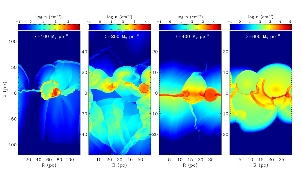
Figure 2.— Density of Series S models at times $t/t_{\rm orb}\approx$2.

Figure 2 shows the volume densities of the four Series S models at two orbital times (2$t_{\rm orb}$) from the start of the simulation. As we discuss below, each model approaches a statistical equilibrium well before $t_{\rm orb}$: the star formation rate, vertical velocity dispersion, disk thickness, and other dynamical-state parameters all approach quasi-steady values. Numerous evolved SN shells are evident in Figure 2. One clear trend in Series S is that in models with higher gas surface density, the gas is also more concentrated towards the midplane (note that the panels have different dimensions).

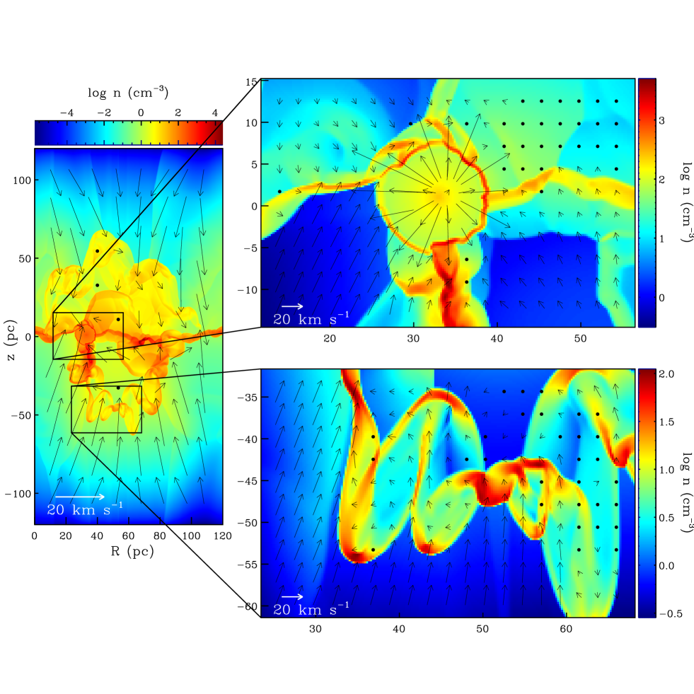
Figure 3.— Densities of model S100 at time $t=2.7t_{\rm orb}$=170 Myr. Vectors show radial-vertical velocities $(v_{R}^{2}+v_{z}^{2})^{1/2}$. White vectors displayed in the bottom left of each panel show the vector scale. Dots indicate locations where the velocity is $<$ 3 km s^-1. The large box is $120\,{\rm pc}\times 240\,{\rm pc}$, and the inset boxes are each $45\,{\rm pc}\times 29\,{\rm pc}$.

The SN feedback events occur in the dense gas near the midplane, and are responsible for pushing gas to higher altitudes, as well as driving turbulence (both horizontal and vertical motions) and creating the filamentary features easily identifiable in Figure 2. Figure 3 shows the density of model S100 at $t=2.7t_{\rm orb}$ = 170 Myr, along with the velocities in the $R,z$ plane. The large scale velocities are generally directed towards the midplane at this particular instant (although at other times the overall flow is expanding, e.g. see Walters & Cox 2001).

A close-up of two regions shows the detailed density and velocity structure. One region focuses on a patch in the midplane where a SN has recently exploded. The vector field illustrates how gas within the SN shell is rapidly expanding away from the center of the bubble, even while surrounding gas is converging. The other close-up shows a region away from the midplane. The dense regions and filamentary structures evident here were created by interactions of gas driven by numerous earlier feedback events. Gas velocities near these dense structures deviate from the large scale converging flow towards the disk midplane. Feedback events thus influence gas motions far from their origin, driving turbulence throughout the simulation domain.

In each model, the star formation rate $\Sigma_{\rm SFR}$ at time $t$ is computed from the number of feedback events $N_{\rm SN}$ occurring over time interval $\Delta t_{\rm bin}$ centered on $t$. The contribution of mass to $\Sigma_{\rm SFR}$ is $N_{\rm SN}$$m_{*}$, where $m_{*}$ is the mass of all stars formed per star capable of undergoing a supernova. Since the star formation probability assumes an effective thickness of our simulation slice $L_{\rm\phi}$= 2$R_{\rm sh}$, the same effective thickness is used in computing the area of the domain projected on the horizontal plane, $L_{\rm R}$$L_{\rm\phi}$. Thus, $\Sigma_{\rm SFR}$ over a given time interval is

$$\Sigma_{\rm SFR}=\frac{m_{*}N_{\rm SN}}{L_{\rm R}L_{\rm\phi}\Delta t_{\rm bin}}.$$ (6)

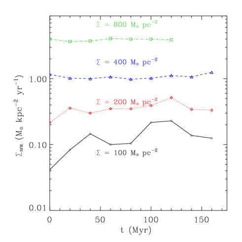
Figure 4.— The evolution of $\Sigma_{\rm SFR}$ with time for Series S models with gas surface densities $\Sigma$= 100 (black circles), 200 (red diamonds), 400 (blue triangles), and 800 (green squares) M_⊙ pc^-2. Points show $\Sigma_{\rm SFR}$ in temporal bins of $\Delta t_{\rm bin}$=20 Myr, as computed from Equation (6).

Figure 4 shows the evolution of $\Sigma_{\rm SFR}$, computed in bins of $\Delta t_{\rm bin}$=20 Myr, as a function of time from all the Series S models. This value of $\Delta t_{\rm bin}$ is much larger than the vertical crossing time of each simulation, which is simply the thickness $H$ of the disk divided by the characteristic vertical velocity $v_{z}$, both of which are defined and analyzed below. We can thus be sure that the estimated $\Sigma_{\rm SFR}$ is averaged over a sufficiently long time such that (on average) gas has cycled between the mid-disk $z=0$ and out-of-plane $|z|>0$ locations numerous times. Figure 4 indicates that $\Sigma_{\rm SFR}$ saturates within 50 Myr, and as we discuss below in Section 3.4, the saturated value generally approaches the predictions from self-regulation.

Figure 5.— The evolution of (a) vertical velocity dispersion $\sigma_{v}$ (see Equation 7), (b) gas disk thickness $H$ (see Equation 8) (c) mean midplane density $n_{\rm 0}$, and (d) mean star formation efficiency $\epsilon_{\rm ff}(n_{\rm 0})$ (see Equation 9), for the S200 model, averaged in 10 Myr temporal bins.

Two quantities describing the gas kinematics and disk structure are the velocity dispersion and disk thickness, respectively. To quantify the vertical motions, we compute the mass-weighted $\hat{z}$-velocity dispersion through

$$\sigma_{v}\equiv\left[\frac{\sum\rho v_{z}^{2}}{\sum\rho}\right]^{1/2},$$ (7)

where the summation is taken over all zones in the simulation. Figure (5a) shows the evolution of the velocity dispersion for model S200. As does $\Sigma_{\rm SFR}$, $\sigma_{v}$ also statistically converges, in this case to $\sim$4.5 km s^-1. Similarly, the mass-weighted disk thickness is defined as

$$H\equiv\langle z^{2}\rangle^{1/2}=\left[\frac{\sum\rho z^{2}}{\sum\rho}\right]^{1/2}.$$ (8)

Higher surface (and volume) densities lead to thinner disks, as evident in Figure 2. Figure (5b) shows that $H$ for model S200 saturates at $\sim$ 9 pc.

Given the vertical velocity dispersion and thickness, the vertical dynamical time is $t_{\rm ver}=H/\sigma_{z}\approx$ 2 Myr for model S200. The measured quantities in Figure 5 are the mean values in 10 Myr bins, so that each bin corresponds to $\sim 5$ dynamical times. Again, this allows sufficient time for gas to cycle between the dense and diffuse phases.

Another quantity of interest is $\epsilon_{\rm ff}(n_{\rm 0})$, the efficiency of star formation per free-fall time, where $t_{\rm ff}(n_{0})$ is evaluated at the mean midplane density $n_{0}$. As discussed in Paper I, $\epsilon_{\rm ff}(n_{\rm 0})$ represents the overall efficiency of star formation at the prevailing ISM conditions, and need not be the same as the value $\epsilon_{\rm ff}(n_{\rm th})$ imposed to set the rate of star formation in very high density gas (see Sections 3.4 and 4).

Since the star formation rate can be directly measured through Equation (6), and $t_{\rm ff}(n_{0})$ can be calculated from the (horizontally- and time- averaged) midplane density $n_{\rm 0}$ measured in the simulations, the mean measured star formation efficiency is given by:

$$\epsilon_{\rm ff}(n_{\rm 0})\equiv\Sigma_{\rm SFR}t_{\rm ff}(n_{\rm 0})/\Sigma.$$ (9)

Figure (5c) and (5d) respectively show the evolution of the midplane density, $n_{\rm 0}$, and the mean efficiency, $\epsilon_{\rm ff}(n_{\rm 0})$, for model S200. As with $\sigma_{v}$ and $H$, these quantities also saturate, with steady-state values $n_{\rm 0}$=385 cm^-3 and $\epsilon_{\rm ff}(n_{\rm 0})$=0.0041.

Figure 6.— Mass-weighted density PDFs for Series S models. The histograms show the average PDFs of densities at 5 Myr intervals, from times 50 Myr $<t<$ 150 Myr. The solid lines show the best fit log-normal distribution. The means (standard deviations) for these mass-weighted log($n$) histograms in models S100, S200, S400, and S800 are, respectively, 2.04 ($\pm$0.81), 2.83 ($\pm$0.80), 3.02 ($\pm$0.69), and 3.51 ($\pm$0.55).

Figure 7.— Mass-weighted vertical-velocity PDFs for Series S models. The histograms show the mass-weighted velocity distributions taken at 5 Myr intervals, from times 50 Myr $<t<$ 150 Myr. The solid lines show the best fit normal distribution. The means (standard deviations) of these mass-weighted $v_{z}$ histograms in models S100, S200, S400, and S800 are, respectively, -0.24 ($\pm$3.45), -0.12 ($\pm$3.92), -0.10 ($\pm$4.82), -0.03 ($\pm$5.67) km s^-1.

Figures 6 and 7 show the mass-weighted density and velocity probability distribution functions (PDFs) for Series S models. The distributions show the average PDFs from times 50 Myr $<t<$ 150 Myr, assessed in 5 Myr intervals. The simulations with higher surface densities produce PDFs which are systematically shifted towards larger volume densities. For model S800, the magnitude of the (self-gravitational and external) potential strongly confines gas to the disk midplane, such that the disk thickness becomes comparable to our chosen value of the SN shell radius $\approx$5 pc (see Fig. 2). The feedback events produce thin shells of shocked gas that have very high densities, which result in the high-density secondary peak. Yet, most of the mid-disk has density  $\buildrel<\over{\sim}$  5000 cm^-3, corresponding to the main peak in Figure 6d. Apart from the S800 model, these density PDFs are all well represented as log-normals, as expected for highly compressible turbulent flows (e.g. Vazquez-Semadeni, 1994; Klessen, 2000; Ostriker et al., 2001). The mass-weighted velocity PDFs are approximately normal, but have more pronounced tails at both high and low velocities. The velocity PDFs do not show any significant differences among the Series S models, indicating that turbulent velocities are not strongly dependent on $\Sigma$ (or $\Sigma_{\rm SFR}$), a point we return to in Section 3.4.

Table 3Characteristics of Hydrodynamic Models

Model	$\Sigma_{\rm SFR}$	$\sigma_{v}$	$H$	$n_{0}$	$\epsilon_{\rm ff}(n_{\rm 0})$	$f_{p}$	$\chi$
	(${\rm M}_{\odot}\,{\rm kpc}^{-2}\,{\rm yr}^{-1}$)	(km s-1)	(pc)	(cm-3)
Series S	(variation in $\Sigma$)
S100	0.15	4.0	11	161	0.0051	0.65	0.054
S200	0.38	4.5	8.8	385	0.0041	1.1	0.069
S400	1.1	5.2	6.5	861	0.0039	1.5	0.090
S800	4.0	5.1	4.4	2157	0.0045	1.6	0.085
Series E	(variation in $\epsilon_{\rm ff}(n_{\rm th})$)
E0.005	0.38	4.5	8.8	385	0.0041	1.1	0.069
E0.01	0.28	5.3	11	278	0.0037	1.5	0.093
E0.025	0.36	6.6	15	177	0.0058	1.2	0.13
E0.05	0.58	7.9	20	140	0.012	0.79	0.19
Series PA	(variation in $p_{*}$)
PA1.5	0.34	2.6	4.5	232	0.0097	0.56	0.024
PA3	0.15	4.0	11	161	0.0051	0.65	0.054
PA6	0.031	6.4	26	60.5	0.0017	1.7	0.13
PA9	0.022	8.0	31	51.5	0.0013	1.8	0.19
Series PB	(variation in $p_{*}$)
PB1.5	0.86	2.8	4.6	516	0.0081	0.90	0.027
PB3	0.28	5.3	11	278	0.0036	1.5	0.093
PB6	0.30	9.0	23	126	0.0055	0.82	0.22
PB9	0.17	12	35	76	0.0040	1.1	0.37
Series O	(variation in $\Omega$)
O1	0.25	4.6	9.5	352	0.0028	1.5	0.019
O2	0.38	4.5	8.8	385	0.0041	1.1	0.069
O4	0.45	4.6	7.4	420	0.0046	1.1	0.24
O8	No collapse/feedback

Table 3 summarizes the mean values $\Sigma_{\rm SFR}$, $\sigma_{v}$  $H$, $n_{\rm 0}$  and $\epsilon_{\rm ff}(n_{\rm 0})$  for all models. Averages are based on bins of 20 Myr, starting at $t=$ 50 Myr. The last two columns give $f_{p}$ and $\chi$, quantities relevant for the analytical expressions derived in Paper I and discussed below. All models with entries listed for the measured parameters reach a steady state. However, Model O8 did not collapse to reach high densities; we believe this is because it is stabilized by a high rotation rate (see Sec. 3.4). In the following section, we compare the properties of each of the simulations presented in Table 3 to the analytical predictions from self-regulation derived in Paper I.

3.4. Comparison with Predictions from Self-Regulation

As discussed in Paper I, in self-regulated starburst regions, the vertical weight $W$ of the molecular disk is expected to be balanced mainly by turbulent pressure $P_{\rm turb}$ (unless the optical depth to IR exceeds $\sim 16$). Under this framework, turbulence is driven predominantly by feedback from massive stars, so the momentum injection rate determines $P_{\rm turb}$. The total upward momentum per unit time per unit area is then given by $f_{p}P_{\rm drive}$ for $P_{\rm drive}$ a fiducial momentum injection rate per unit area associated with star formation and $f_{p}$ an order-unity dimensionless constant. Each of the gravitational, turbulent, and feedback momentum-injection fluxes may be measured directly in the simulations through:

$$W=\frac{\pi G\Sigma^{2}}{2}(1+\chi),$$ (10)

$$P_{\rm turb}=\rho_{0}\sigma_{v}^{2},$$ (11)

$$P_{\rm drive}=\frac{1}{4}\frac{p_{*}}{m_{*}}\Sigma_{\rm SFR},$$ (12)

respectively. As discussed below, $\chi$ accounts for the gravity of the stellar bulge relative to gas self-gravity, and is usually small. In choosing a fiducial value for $p_{*}$ we assume that radiative supernova shells dominate the momentum injection (see Equation 5), but other terms could equally well be included in Equation (12), and we explore a range of $p_{*}$. If the disk evolves to be turbulence-dominated and governed by star formation self-regulation, then we should find that $P_{\rm turb}$$\approx$ $P_{\rm drive}$$\approx W$.

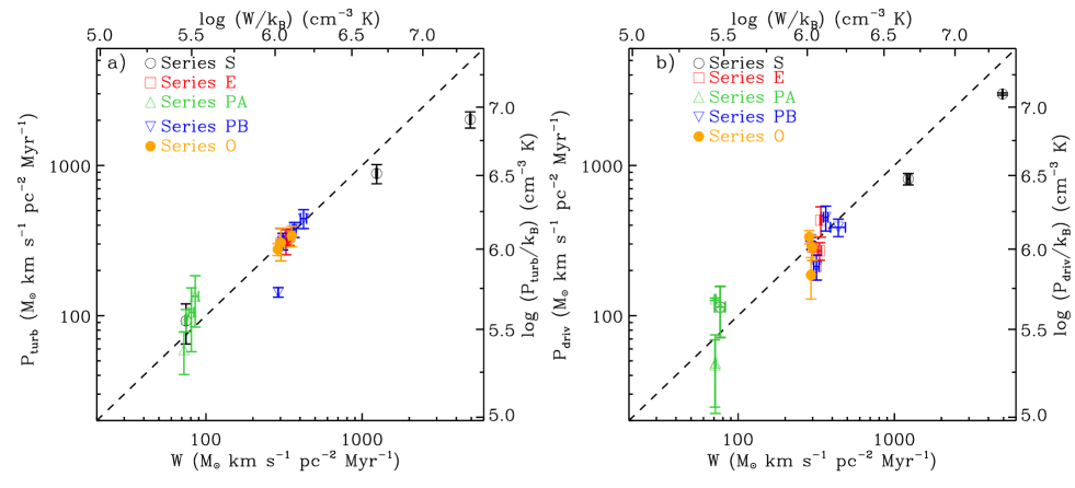
Figure 8.— Momentum fluxes (a) $P_{\rm turb}$ and (b) $P_{\rm drive}$ plotted against vertical weight of gaseous disk $W$ from each simulation (see Equations 10 - 12). Each point indicates the mean values of the momentum fluxes measured in 20 Myr bins, after the simulations reach a steady state ($\approx$1 $t_{\rm orb}$). The error bars show the (1$\sigma$) standard deviations. The dashed lines show the expectation from vertical equilibrium with self-regulation, where $P_{\rm turb}$ $\approx W\approx$ $P_{\rm drive}$.

Figure 8 shows the relationships of the measured momentum fluxes $P_{\rm turb}$ and $P_{\rm drive}$ with $W$. We compute $P_{\rm turb}$ in the simulations using midplane horizontal- and time-averages of $\langle\rho v_{z}^{2}\rangle$. The turbulent and SN momentum fluxes are in excellent agreement with the vertical weight of the disk. For those models showing the largest deviation from the expectations in Figure (8a), simulations PB1.5 and S800, there is only a factor of two discrepancy between $P_{\rm turb}$ and $W$. In Figure (8b), models S400 and S800 have the largest discrepancy between the predicted and measured momentum injection rates. For very strong gravity models, the disk thickness becomes comparable to the (imposed) radii of SN shells in our models. As a consequence, the disk can become “artificially” thickened, because real feedback shells starting at much smaller radii and conserving momentum might not expand as much. If shells reach larger sizes than their “natural” radii, the corresponding mean density and pressure would be somewhat lower than would be required for self-regulated equilibrium. Overall, the general correspondence between $P_{\rm turb}$, $P_{\rm drive}$, and $W$ strongly supports the idea that the evolution of our ISM models reaches an equilibrium governed by star formation self-regulation. To further explore this premise, we now turn our attention to comparing other physical properties of the simulations with the predictions from self-regulation theory.

We begin by providing an overview of the analytical results expected under self-regulation. The star formation rate in equilibrium is obtained by equating $f_{p}P_{\rm drive}\equiv P_{\rm turb}$ with $W$ (Equation 13 in Paper I):

$$\Sigma_{\rm SFR} = \frac{2\pi(1+\chi)}{f_{p}}\frac{m_{*}G\Sigma^{2}}{p_{*}}$$ (13)

$$= 0.092\,{\rm M_{\odot}\,kpc^{-2}\,yr^{-1}}\left(\frac{\Sigma}{100\,{\rm M_{\odot}\,pc^{-2}}}\right)^{2}$$

$$\times\frac{(1+\chi)}{f_{p}}\left(\frac{p_{*}/m_{*}}{3000\,{\rm\,km\,s^{-1}}}\right)^{-1}.$$

The factor $\chi$ accounts for the gravitational potential due to the bulge (see Section 2 and 4 in Paper I), with

$$\chi=\frac{2C}{1+\sqrt{1+4C}}.$$ (14)

Here, $C\approx 0.66\mathcal{W}^{2}$, where $\mathcal{W}=\sigma_{v}\Omega/(\pi G\Sigma)$ is a parameter analogous to the Toomre $Q$ parameter (Toomre, 1964). Using typical values,

$$C=0.35\left[\left(\frac{\sigma_{v}}{{\rm 10km\,s^{-1}}}\right)\left(\frac{\Omega}{0.1\,{\rm Myr}^{-1}}\right)\left(\frac{\Sigma}{100\,{\rm M_{\odot}\,pc}^{-2}}\right)^{-1}\right]^{2};$$ (15)

thus $C$ is typically small in our simulations.

The parameter $f_{p}$ characterizes the magnitude of turbulent dissipation, with $f_{p}\sim 1$ for strong dissipation and $f_{p}\sim 2$ for weak dissipation. The value of $f_{p}$ is defined by the ratio of $P_{\rm turb}$ and the fiducial vertical momentum flux injected by star formation, $P_{\rm drive}$ (see Equations 11 - 12):

$$f_{p} \equiv P_{\rm turb}\left(\frac{p_{*}}{4m_{*}}\Sigma_{\rm SFR}\right)^{-1}$$ (16)

$$= W\left(\frac{p_{*}}{4m_{*}}\Sigma_{\rm SFR}\right)^{-1},$$ (17)

where the second line assumes that dynamical equilibrium also holds (see Fig. 8, as well as Fig. 8 of KKO11). Accordingly, in a self-regulated system,

$$f_{p} = 0.92\,(1+\chi)\,\left(\frac{\Sigma_{\rm SFR}}{\rm 0.1M_{\odot}\,kpc^{-2}\,yr^{-1}}\right)^{-1}\left(\frac{\Sigma}{100\,{\rm M_{\odot}\,pc^{-2}}}\right)^{2}$$ (18)

$$\times\left(\frac{p_{*}/m_{*}}{3000{\rm km\,s^{-1}}}\right)^{-1};$$

this is a simply a re-arrangement of Equation (13). We note that $P_{\rm turb}=\rho_{0}\sigma_{v}^{2}$ is equivalent to $(\Sigma\sigma_{v}/2)(H/\sigma_{v})^{-1}$. With $\Sigma\sigma_{v}/2$ the vertical momentum per unit area contained in each side of the disk, and $H/\sigma_{v}$ the vertical crossing time, the relation $P_{\rm turb}\approx P_{\rm drive}$, or $f_{p}\approx 1$, thus implies that the disk’s vertical momentum is replenished by feedback approximately once per dynamical time.

Using the value of $\Sigma_{\rm SFR}$ measured using Equation (6) and $\chi$ from Equation (14), we can calculate $f_{p}$ in each simulation from Equation (18). To obtain $\chi$ through Equations (14) and (15), we use the measured value of $\sigma_{v}$. Table 3 provides the values of $f_{p}$ measured from the simulations in this way; all values are near unity. We have verified that $f_{p}$ measured through Equation (16) provides similar values, since $P_{\rm turb}$ $\approx W$ (Fig. 17). Table 3 also shows that $\chi$ is measured to be rather small.

By equating $P_{\rm turb}$ and $W$, the turbulent velocity dispersion can be expressed as a relationship between the characteristic vertical acceleration under self-gravity, $\sim\sigma_{v}/t_{\rm ff}$, and the mean gravitational field $\approx\pi G\Sigma$:

$$\sigma_{v} = \frac{4}{\sqrt{3}}t_{\rm ff}(n_{\rm 0})G\Sigma(1+\chi)^{1/2}$$ (19)

$$= 4.42\,{\rm km\,s}^{-1}\left(\frac{n_{0}}{100\,{\rm cm}^{-3}}\right)^{-1/2}\left(\frac{\Sigma}{100\,{\rm M_{\odot}\,pc}^{-2}}\right)$$

$$\times(1+\chi)^{1/2}.$$

Equation (19) should hold for any disk-like system supported primarily by turbulence, independent of the source of that turbulence.

The predicted velocity dispersion $\sigma_{v}$ can also be expressed in terms of $\epsilon_{\rm ff}(n_{\rm 0})$, $f_{p}$, and $\chi$ as:

$$\sigma_{v}=5.5\,{\rm km\,s^{-1}}\frac{f_{p}}{(1+\chi)^{1/2}}\left(\frac{\epsilon_{\rm ff}(n_{0})}{0.005}\right)\left(\frac{p_{*}/m_{*}}{3000\,{\rm\,km\,s^{-1}}}\right)$$ (20)

(see Equation 22 of Paper I); Equation (20) follows from Equation (19) using the definitions of $\epsilon_{\rm ff}(n_{\rm 0})$ and $f_{p}$ from Equations (9) and (18), respectively. This form shows that if $f_{p}$ and $\epsilon_{\rm ff}(n_{\rm 0})$ are approximately constant, then the velocity dispersion would be proportional to the momentum/mass injected by star formation.

Lastly, the predicted disk thickness $H$ when dynamical equilibrium holds is:

$$H = \frac{1}{1+\chi}\frac{\sigma_{v}^{2}}{\pi G\Sigma}$$ (21)

$$= 74\,{\rm pc}\frac{1}{1+\chi}\left(\frac{\sigma_{v}}{10\,{\rm\,km\,s^{-1}}}\right)^{2}\left(\frac{\Sigma}{100\,{\rm M_{\odot}\,pc^{-2}}}\right)^{-1}.$$

(Note that the first equality in Equation 28 of Paper I contains a typo; the denominator should contain a $\Sigma$ instead of a $\Sigma^{2}$.) Using Equation (20), this may be re-expressed as

$$H = 23\,{\rm pc}\,\frac{f_{p}^{2}}{(1+\chi)^{2}}\left(\frac{\epsilon_{\rm ff}(n_{0})}{0.005}\right)^{2}$$

$$\times\left(\frac{p_{*}/m_{*}}{3000\,{\rm\,km\,s^{-1}}}\right)^{2}\left(\frac{\Sigma}{100\,{\rm M_{\odot}\,pc^{-2}}}\right)^{-1}.$$

When the definitions for $\epsilon_{\rm ff}(n_{\rm 0})$ and $f_{p}$ (Equations 9 and 18) are substituted into Equation (LABEL:Hpred), the result is $\Sigma/(2\rho_{0})$. While Equation (21) should hold independent of the source of turbulence, Equation (LABEL:Hpred) shows that $H$ would scale inversely with $\Sigma$ for self-regulated turbulent disks if $f_{p}$ and $\epsilon_{\rm ff}(n_{\rm 0})$ remain approximately constant.

Using the measured values of $\Sigma_{\rm SFR}$, $\sigma_{v}$, $H$, and $n_{\rm 0}$ in each simulation, we can test a number of aspects of the theory in Paper I. In particular, we can: (1) compare our measurements of $\Sigma_{\rm SFR}$ to Equation (13) to assess the combined (turbulent driving/dissipation and gravity/pressure) equilibrium and test whether $f_{p}\sim 1$ is satisfied (for varying physical parameters $\Sigma$, $p_{*}$, $\Omega$ and varying numerical parameter $\epsilon_{\rm ff}(n_{\rm th})$); (2) compare our measurements of $\sigma_{v}$ to Equation (19) to assess the balance of turbulent pressure and weight, also comparing to Equation (20) to evaluate whether $f_{p}$ and $\epsilon_{\rm ff}(n_{\rm 0})$ are effectively constant (for varying parameters); (3) compare our measurements of $H$ to Equation (21) to assess dynamical equilibrium, also comparing to Equation (LABEL:Hpred) to evaluate whether $f_{p}$ and $\epsilon_{\rm ff}(n_{\rm 0})$ are effectively constant (for varying parameters). In addition, we can (4) use our measurements of $\Sigma_{\rm SFR}$ and $n_{\rm 0}$ to compute a measured $\epsilon_{\rm ff}(n_{\rm 0})$ via Equation (9) and explore whether there are any systematic dependencies on the physical or numerical parameters.

Figure 9 shows the mean $\Sigma_{\rm SFR}$ for all models after a steady state is reached (generally $t>50$ Myr). The star formation rate is plotted against the main user-defined parameters varied between models from each series, a) $\Sigma$ (Series S), b) $\epsilon_{\rm ff}(n_{\rm th})$ (Series E), c) $p_{*}$ (Series PA and PB), and d) $\Omega$ (Series O). The dashed lines in each panel show the predictions from self-regulation theory (Equation 13), for $f_{p}$ = 0.5 and 1.5, and with $\chi$=0.

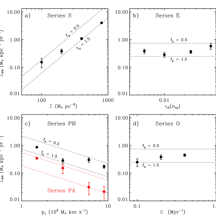
Figure 9.— Mean $\Sigma_{\rm SFR}$ from the simulations (points), and that predicted from self-regulated equilibrium (lines), for two different values of $f_{p}$ = 0.5 and 1.5 (see Equation 13). $\Sigma_{\rm SFR}$ is plotted against the model input parameter that is varied in each series: a) gas surface density $\Sigma$, b) star formation efficiency in dense gas $\epsilon_{\rm ff}(n_{\rm th})$, c) momentum input per high mass star $p_{*}$, and d) local angular rotational velocity $\Omega$ (which also affects the vertical gravity). Error bars show the 1$\sigma$ deviation of the measured $\Sigma_{\rm SFR}$.

For Series S, Figure 9a shows a remarkably good agreement between the measured star formation rate and the prediction for $f_{p}\sim 1$. Although the increase of $\Sigma_{\rm SFR}$ with $\Sigma$ for Series S is slightly shallower than the power predicted in Equation (13) (1.6 vs. 2), a larger adopted $\epsilon_{\rm ff}(n_{\rm th})$ leads to a slightly steeper slope, so that our overall results are generally consistent with $\Sigma_{\rm SFR}\propto\Sigma^{2}$ (see Fig. 4 of Paper I).

Equation (13) indicates that $\Sigma_{\rm SFR}$ under self-regulation is independent of the star formation efficiency in dense gas. Figure 9b indeed shows that the measured value of $\Sigma_{\rm SFR}$ for Series E models is relatively insensitive to the chosen value of $\epsilon_{\rm ff}(n_{\rm th})$. Physically, this means that (within limits) the rate of star formation in dense gas does not affect the overall star formation rate averaged over large scales, because the amount of mass at high density simply adjusts until the feedback rate matches what is required to produce the needed turbulent pressure.

From Equation (13), the star formation rate in self-regulated equilibrium should be inversely proportional to the input momentum per stellar mass $p_{*}/m_{*}$, where $p_{*}$ is associated with high-mass stars and $m_{*}$ includes all of the lower-mass stars proportionally (based on the IMF). Figure 9c shows $\Sigma_{\rm SFR}$ as a function of $p_{*}$ for Series PA and PB models. An inverse proportionality between $\Sigma_{\rm SFR}$ and $p_{*}$ is evident, comparing favorably to the prediction from self-regulation.

The rate of star formation in a self-regulated system is not expected to depend on the angular velocity $\Omega$, provided that angular momentum does not limit local collapse (i.e. on scales  $\buildrel<\over{\sim}$ $H$) and that the vertical stellar gravity is small compared to the vertical gas gravity (i.e. $\chi\ll 1$). The independence of $\Sigma_{\rm SFR}$ from $\Omega$ is shown in Figure 9d. We found, however, that when $\Omega$ is large enough – as in Model O8, angular momentum prevents clouds from collapsing to reach high densities ($n_{\rm th}$ = 5000 cm^-3), and we register it as non-star-forming. This model has Toomre wavelength $\lambda_{T}=\pi^{2}G\Sigma/\Omega^{2}\approx$ 14 pc. This value of $\lambda_{T}$ is comparable to what would otherwise be the collapse scale, thereby stabilizing the ISM and preventing the formation of any clouds.

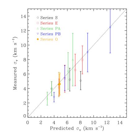
Figure 10.— The measured and predicted values of the velocity dispersion $\sigma_{v}$ for all models, as defined in Equations (7) and (19), respectively. The agreement between the measured and predicted dispersion shows that dynamical equilibrium between gravity and turbulent pressure is established.

Figure 10 shows how $\sigma_{v}$ as measured in each simulation (Equation 7) compares to the expectation from vertical dynamical equilibrium (Equation 19). There is generally a good correspondence between the predicted and measured values. This comparison contains essentially the same information as in Figure (8a), and similar to the results there, the measured $\sigma_{v}$ for a few models depart somewhat from the prediction. The greatest departure is for model S800, which is expected since the disk thickness approaches the numerically-imposed feedback shell size.

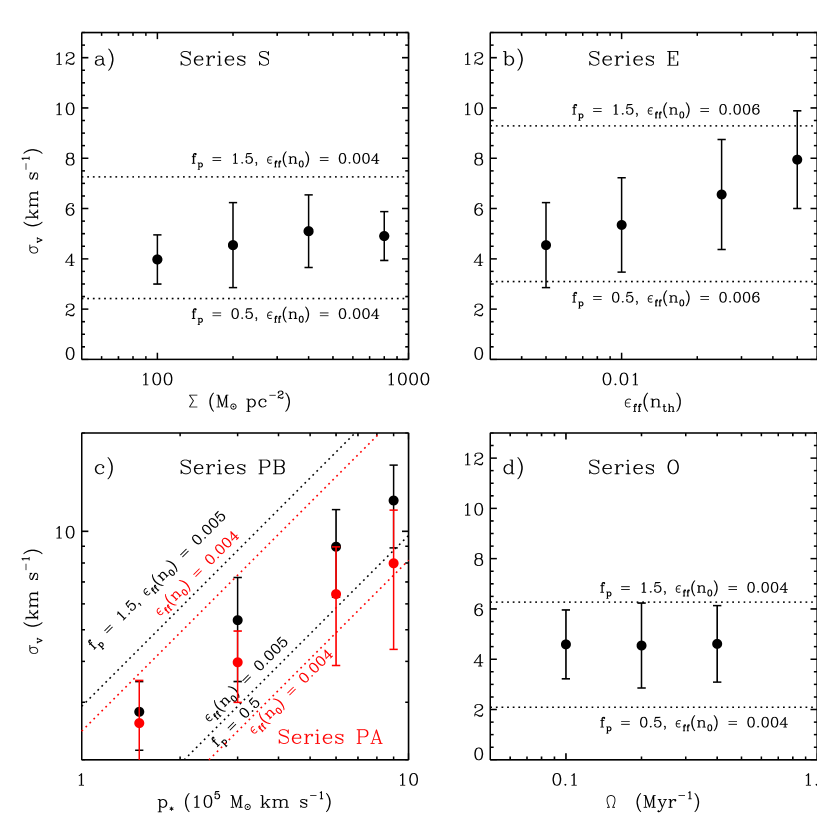
Figure 11.— Mean vertical velocity dispersion $\sigma_{v}$ (see Equation 7) from simulations (points), along with the prediction from self-regulation (lines), assuming the mean value of $\epsilon_{\rm ff}(n_{\rm 0})$ for each Series and with $f_{p}$=0.5 and 1.5 (see Equation 20). The panels separately show each series, i.e. $\sigma_{v}$ against a) $\Sigma$, b) $\epsilon_{\rm ff}(n_{\rm th})$  c) $p_{*}$, and d) $\Omega$. Error bars show the 1$\sigma$ deviation of the measured $\sigma_{v}$.

Figure 11 shows $\sigma_{v}$ measured in the simulations for each series. The dashed lines in each panel indicate the prediction from self-regulation given by Equation (20), again with $f_{p}=$0.5 and 1.5, along with $\chi$=0, and using the mean value of $\epsilon_{\rm ff}(n_{\rm 0})$ for each series. The predicted independence of $\sigma_{v}$ from $\Sigma$ and $\Omega$ is confirmed in Figures 11a and 11d, respectively.

Figures 11b-c indicate that the measured $\sigma_{v}$ increases with $\epsilon_{\rm ff}(n_{\rm th})$ and $p_{*}$, respectively. In Figure 11b, the lines correspond to Equation (20) with constant $\epsilon_{\rm ff}(n_{\rm 0})$=0.006. However, as discussed below, the measured $\epsilon_{\rm ff}(n_{\rm 0})$ increases with $\epsilon_{\rm ff}(n_{\rm th})$ (also evident in Table 3), implying from Equation (20) that $\sigma_{v}$ should indeed increase with $\epsilon_{\rm ff}(n_{\rm th})$. Similarly, Figure 11c shows that the increase in $\sigma_{v}$ with $p_{*}$ is shallower than the linear relation indicated in Equation (20) for constant $\epsilon_{\rm ff}(n_{\rm 0})$. This is due to the slight decrease in $\epsilon_{\rm ff}(n_{\rm 0})$ with $p_{*}$, which is further discussed below.

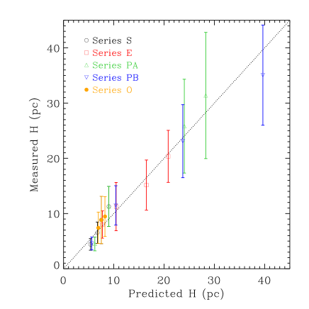
Figure 12.— The measured and predicted values of the disk thickness $H$ for all models, as defined in Equations (8) and (21), respectively. The agreement between the measured and predicted thickness indicates vertical equilibrium between the weight due to gravity and SN driven turbulent pressure.

Figure 12 compares the measured and predicted values of $H$, given by Equation (8) and (21) respectively. As with the velocity dispersion (Fig. 10), the thickness is measured to be very similar to the predicted value. This agreement is indicative of vertical equilibrium between the weight due to gravity and turbulent pressure.

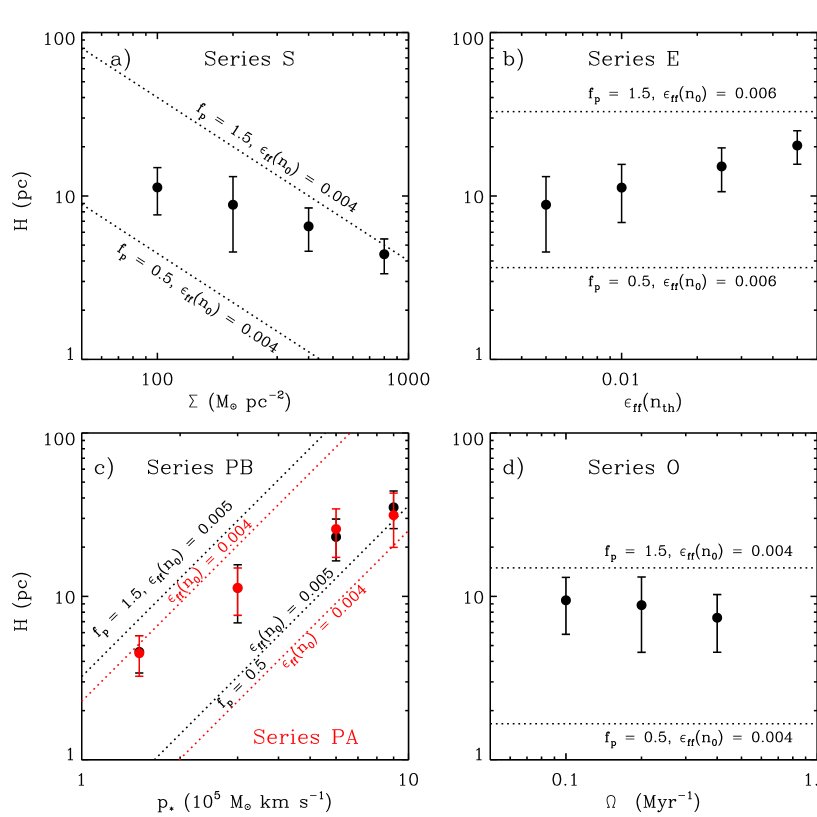
Figure 13.— Mean disk thickness $H$ (Equation 8) in all models, along with the prediction from self-regulation (lines), assuming the mean value of $\epsilon_{\rm ff}(n_{\rm 0})$ for each Series and with $f_{p}$=0.5 and 1.5 (see Equation LABEL:Hpred). $H$ is plotted against a) $\Sigma$, b) $\epsilon_{\rm ff}(n_{\rm th})$  c) $p_{*}$, and d) $\Omega$. Error bars show the 1$\sigma$ deviation of the measured $H$.

Figure 13 shows the measured thickness $H$ from Equation (8), compared to the prediction from Equation (LABEL:Hpred) for constant $f_{p}$ and $\epsilon_{\rm ff}(n_{\rm 0})$. Figures 13a shows that $H$ decreases with $\Sigma$ less steeply than $\propto\Sigma^{-1}$. Based on Equation (LABEL:Hpred) this is consistent with the systematic increase of $f_{p}$ with $\Sigma$ for Series S (see Table 3). Since the SN shell radius is chosen to be 5 pc in these numerical simulations, this places an effective lower limit on the disk thickness $H$  $\buildrel>\over{\sim}$ 5 pc, which might be part of the reason for the shallow decrease of $H$ with $\Sigma$. Similar to the case of $\sigma_{v}$, the increase of $H$ with $\epsilon_{\rm ff}(n_{\rm th})$ and $p_{*}$ in Figures 13b-c can be fully accounted for by the variation of $\epsilon_{\rm ff}(n_{\rm 0})$ with $\epsilon_{\rm ff}(n_{\rm th})$ and $p_{*}$, respectively. Figure 13d shows that $H$ is insensitive to $\Omega$, implying that neither rotation nor the external gravity of the bulge strongly affects the disk thickness, within the range shown.

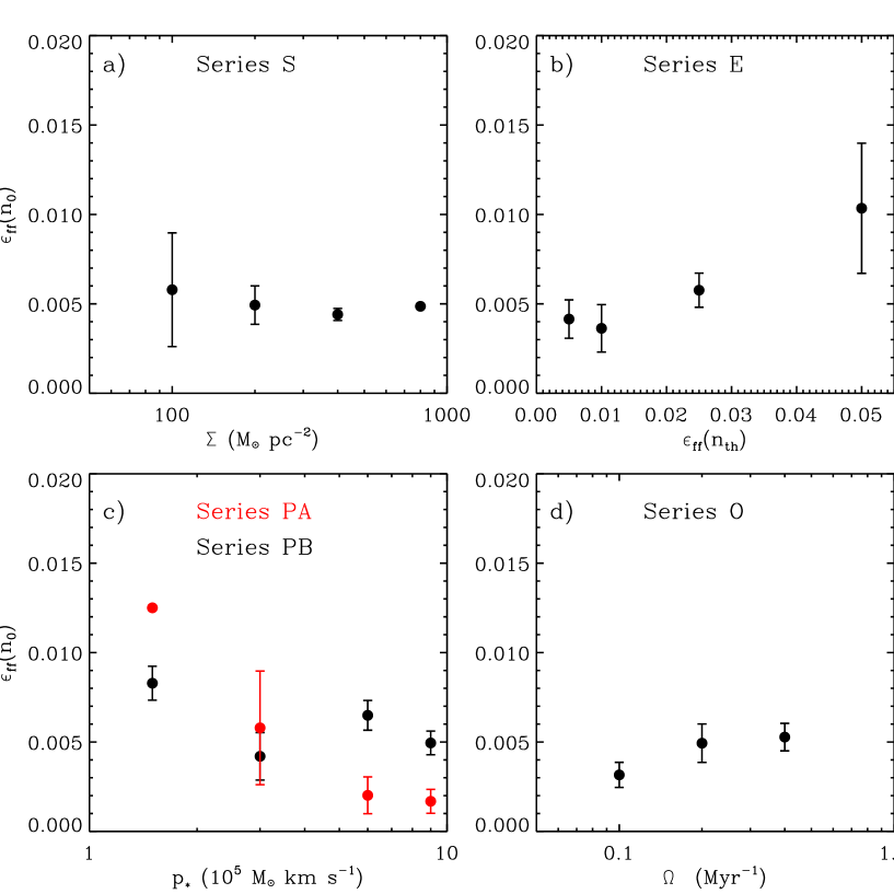
Figure 14.— Calculated star formation efficiency per free-fall time at the midplane density, $\epsilon_{\rm ff}(n_{\rm 0})$, plotted for all models against a) $\Sigma$, b) $\epsilon_{\rm ff}(n_{\rm th})$  c) $p_{*}$, and d) $\Omega$. Error bars show the 1$\sigma$ deviation of the measured $\epsilon_{\rm ff}(n_{\rm 0})$.

The measured value of $\epsilon_{\rm ff}(n_{\rm 0})$, as computed through Equation (9) for each simulation, is shown in Figure 14. In general, there are only slight variations in $\epsilon_{\rm ff}(n_{\rm 0})$ among the simulations; for Series S and O, $\epsilon_{\rm ff}(n_{\rm 0})$ is approximately constant. As discussed above with regard to $\Sigma_{\rm SFR}$, we interpret the weak dependence of $\epsilon_{\rm ff}(n_{\rm 0})$ on $\epsilon_{\rm ff}(n_{\rm th})$ as indicative of an adjustment in the mass of dense gas to meet the large-scale need for star formation feedback. This adjustment is possible because the dynamical timescales decrease with increasing density and decreasing spatial scale. Other recent numerical studies have also found that large-scale star formation rates are insensitive to user-defined parameters controlling star formation at small scales (see section 4.1). Figure 14c demonstrates that $\epsilon_{\rm ff}(n_{\rm 0})$ decreases somewhat with increasing $p_{*}$. Potentially, this may be due to the increase of velocity dispersion with increasing $p_{*}$, which renders a smaller fraction of gas eligible to collapse (see section 4.1).

In summary, based on our quantitative comparisons, the results from our numerical simulations show good agreement with the simple analytic theory of Paper I. Both vertical dynamical equilibrium and a balance between turbulent driving and dissipation are satisfied. The dependence of $\Sigma_{\rm SFR}$, $\sigma_{v}$, and $H$ on the gas surface density $\Sigma$ and input momentum $p_{*}$ are similar to the predicted behavior. In addition, the results are insensitive to the exact prescription for star formation in dense gas. The free parameter $f_{p}$ was introduced in Paper I to characterize the turbulent “yield” from momentum inputs by star formation, and our present simulations provide a numerical evaluation of $f_{p}$. For our whole simulation suite, $f_{p}$ remains within $\sim 50$% of unity, the value for strong dissipation.

4. Discussion and Summary

To investigate dynamics of the highly-turbulent, molecule-dominated ISM as found in (U)LIRGS and galactic centers, we have executed a suite of numerical simulations that incorporate feedback from star formation. We demonstrate that in simulations reaching a steady state, many physical properties can be accounted for by a simple theory of star formation self-regulation (Paper I). Namely, the turbulent pressure is driven by injected SN momentum, and dissipates within a vertical crossing time of the disk. The rate of star formation and momentum injection adjusts until the input rate of momentum flux balances the vertical weight of the gaseous disk.

4.1. Relationship to Previous Work

Our numerical simulations of the ISM are similar in some respects to other recent modeling efforts that have included turbulent driving from localized feedback events, and our results are consistent with previous findings. In particular, we have found that the velocity dispersion $\sigma_{v}$ is not strongly dependent on the the exact prescription for feedback as long as the momentum (or energy) input is similar (Dib et al., 2006; Shetty & Ostriker, 2008; Joung et al., 2009, KKO11). Additionally, we find that the overall star formation rate $\Sigma_{\rm SFR}$ is not sensitive to the chosen value of $\epsilon_{\rm ff}(n_{\rm th})$, in general agreement with the conclusions of Dobbs et al. (2011) and Hopkins et al. (2011) that the specific small-scale star formation prescription does not not strongly affect the resulting $\Sigma_{\rm SFR}$. Similar to previous efforts that have explored a large range of surface densities, our simulations here and in Paper I clearly demonstrate a power law relationship between $\Sigma$ and $\Sigma_{\rm SFR}$ (e.g. Li et al., 2005, 2006; Tasker & Bryan, 2006, 2008; Robertson & Kravtsov, 2008; Shetty & Ostriker, 2008; Dobbs & Pringle, 2009; Koyama & Ostriker, 2009a; Dobbs et al., 2011; Hopkins et al., 2011). Here, our numerical simulations are well resolved in the vertical direction, and we relate both the power law and coefficient of the $\Sigma_{\rm SFR}$ vs. $\Sigma$ relationship to the requirements for equilibrium given in the self-regulation theory of Paper I.

For the high-surface-density regime $\Sigma$ $\buildrel>\over{\sim}$ 100 M_⊙ pc^-2 studied in this work, observations show that the $\Sigma_{\rm SFR}$ vs. $\Sigma$ relationship is steeper than linear. As discussed in Paper I, an accurate calibration of $X_{\rm CO}$, the ratio of gas mass to velocity-integrated CO intensity, is crucial for estimating $\Sigma$ (and thus the exact power law of $\Sigma_{\rm SFR}$ vs. $\Sigma$) from CO observations. Recent theoretical efforts have advanced our understanding of $X_{\rm CO}$, in both Milky-Way like GMCs (e.g. Glover & Mac Low, 2011; Shetty et al., 2011a, b), as well as large scale galaxies and merger systems (e.g. Narayanan et al., 2011, 2012). These models use a combination of numerical hydrodynamic simulations and radiation transfer to assess environmental dependencies of $X_{\rm CO}$.

If gas dominates the vertical gravity, the theory of Paper I results in a power-law relationship $\Sigma_{\rm SFR}$$\propto$ $\Sigma$² (Equation 13); the numerical simulations presented in Paper I and here (Fig. 9) support this model. As demonstrated in Paper I, employing a continuously varying $X_{\rm CO}$ indeed shows $\Sigma_{\rm SFR}$$\propto$ $\Sigma$² for a sample of ULIRGs and the Galactic center (Genzel et al., 2010; Yusef-Zadeh et al., 2009). Narayanan et al. (2012) investigated the relationship between $X_{\rm CO}$ and the velocity integrated CO ($J=1-0$) brightness temperature $W_{\rm CO}$ in a large compilation of low- and high-$z$ galaxies. Applying the model-based calibration $X_{\rm CO}\propto W_{\rm CO}^{-0.3}$, Narayanan et al. (2012) found that $\Sigma_{\rm SFR}\approx 0.1\,{\rm M_{\odot}\,kpc^{-2}\,yr^{-1}}({\Sigma}/{100\,{\rm M_{\odot}\,pc^{-2}}})^{1.95}$, in agreement with the Paper I prediction (Equation 13 here, with $f_{p}\approx 1$ and $\chi\ll 1$).

The self-regulation theory of Paper I has a number of similarities to and differences from the star formation model in the high-surface-density molecule-dominated regime ($\Sigma$ $\buildrel>\over{\sim}$ 100 M_⊙ pc^-2) proposed by Krumholz and coworkers (Krumholz & McKee, 2005; Krumholz et al., 2009, 2012). Both models rely on the role of supersonic turbulence. In Krumholz et al, the specific star formation rate is characterized in terms of an efficiency per free-fall time at the mean density (essentially $\epsilon_{\rm ff}(n_{\rm 0})$), where the mean density (which sets $t_{\rm ff}(n_{0})$) depends on $\Sigma$ and the turbulence level. Krumholz & McKee (2005) argued that this efficiency should depend on the fraction of gas at pressures higher than the mean turbulent pressure, and pointed out that for log-normal density PDFs, this fraction depends only weakly on the Mach number ($\propto{\cal M}^{-0.3}$) and is predicted to be $\sim 0.01$, consistent with observations of molecular gas (Krumholz & Tan, 2007). Krumholz et al. do not, however, directly address the origin of turbulence – i.e. what sets $\sigma_{v}$. Rather, they adopt the assumption that Toomre $Q$ (and therefore $\cal W$) is order-unity, so that $\sigma_{v}\sim\pi G\Sigma/\Omega$, and adopt an empirically-motivated relation $\Omega\propto\Sigma^{0.5}$ (so that $\sigma_{v}\propto\Sigma^{0.5}$) to obtain $\Sigma_{\rm SFR}\propto\epsilon_{\rm ff}\Sigma/t_{\rm ff}\propto\Sigma^{2}/\sigma_{v}^{1.3}\propto\Sigma^{1.3}$.

Although the star formation rate in the current theory can also be characterized in terms of the velocity dispersion and $\epsilon_{\rm ff}(n_{\rm 0})$ (see Equation 21 of Paper I), the fundamental relationship is instead Equation (13). This expression connects the star formation rate to the weight of the ISM (or equilibrium midplane pressure) and to the momentum/mass injected by feedback ($p_{*}/m_{*}$), yielding $\Sigma_{\rm SFR}\approx 2\pi G\Sigma^{2}(p_{*}/m_{*})^{-1}$. Equating this relation to $\Sigma_{\rm SFR}$$\equiv$ $\epsilon_{\rm ff}(n_{\rm 0})$$\Sigma$/$t_{\rm ff}(n_{0})$$\approx(4\epsilon_{\rm ff}(n_{0})/\sqrt{3})G\Sigma^{2}/\sigma_{v}$ then leads to a proportionality between the velocity dispersion and both $\epsilon_{\rm ff}(n_{\rm 0})$ and $p_{*}/m_{*}$ (see Equation 20). Here, we use numerical simulations to evaluate $\epsilon_{\rm ff}(n_{\rm 0})$ (see Fig. 14 and Table 3), finding values in the range $\sim 0.005-0.01$, consistent with Krumholz & McKee (2005) and Krumholz & Tan (2007). We find, however, that the velocity dispersion is essentially independent of $\Sigma$ (see Fig. 11a), which differs from the $\sigma_{v}\propto\Sigma^{0.5}$ relation adopted by Krumholz et al. We note that due to lack of resolution, the molecular velocity dispersion on scales comparable to the disk thickness is difficult to obtain with observations, although this situation will improve with ALMA.

4.2. Summary of Results

We have conducted a suite of simulations in which we independently varied the gas surface density $\Sigma$, the input momentum per high mass star $p_{*}$, the angular rotation rate of the gas $\Omega$, and the efficiency of star formation in very dense gas, $\epsilon_{\rm ff}(n_{\rm th})$. For each simulation, we measured the star formation rate and ISM properties after a statistical steady state developed, and compared to the predictions of Paper I. Our main results are as follows:

[1] For essentially all models, we find excellent correspondence between the turbulent momentum flux $P_{\rm turb}$, the vertical weight of the gaseous disk $W$, and the vertical momentum injection rate per area $P_{\rm drive}$ associated with feedback (Fig. 8). The result that $P_{\rm turb}$ $\approx W\approx$ $P_{\rm drive}$ strongly supports the idea that the combined ISM/star formation system in starburst disks can be self-regulated, as described in Paper I.

[2] Our results (Fig. 9) show that $\Sigma_{\rm SFR}$ is essentially independent of $\Omega$ and $\epsilon_{\rm ff}(n_{\rm th})$, whereas $\Sigma_{\rm SFR}$ increases for higher $\Sigma$ and decreases for higher $p_{*}$ following the expectations of self-regulation theory. The result that the large-scale $\Sigma_{\rm SFR}$ is independent of the star formation rate in dense gas means that the processes with the longest timescales (associated with the largest spatial scales) are what controls the overall star formation rate. Physically this makes sense: gas that reaches high density collapses rapidly, but the (slower) rate at which this dense gas is resupplied by lower-density gas depends on larger-scale dynamics. As noted in Paper I (see also Narayanan et al., 2012), the prediction $\Sigma_{\rm SFR}\approx 0.1\,{\rm M_{\odot}\,kpc^{-2}\,yr^{-1}}({\Sigma}/{100\,{\rm M_{\odot}\,pc^{-2}}})^{2}$ of Equation (13) also agrees with observations provided that $X_{\rm CO}$ decreases modestly with increasing $\Sigma$ (or $W_{\rm CO}$).

[3] We find that the star formation efficiency per free-fall time at the mean midplane density, $\epsilon_{\rm ff}(n_{\rm 0})$, is independent of $\Sigma$, $\Omega$, and $\epsilon_{\rm ff}(n_{\rm th})$, and decreases only slightly with increasing $p_{*}$. The resulting $\epsilon_{\rm ff}(n_{\rm 0})$$\sim 0.005-0.01$ is similar to the theoretical estimates for turbulent, self-gravitating gas at high Mach number of Krumholz & McKee (2005), while being somewhat lower than the numerical estimates (from turbulent simulations with periodic boundary conditions) of Padoan & Nordlund (2011). Measured ratios of the stellar-to-gas content in nearby molecular clouds are $\sim 0.03-0.06$ (Evans et al., 2009), which would imply similar $\epsilon_{\rm ff}(n_{\rm 0})$ to our results if the cloud ages are several free-fall times. Gas at more extreme conditions in ULIRGs is also observed to have $\epsilon_{\rm ff}(n_{\rm 0})$$\sim 0.01$ (Krumholz & Tan, 2007).

[4] The vertical velocity dispersions in our models are in the range $\sigma_{v}\in 3-12$ km s^-1 for momentum per high mass star in the range $p_{*}\in 1.5-9\times 10^{5}$ M_⊙  km s^-1. Similar to previous results, we find that $\sigma_{v}$ is relatively independent of $\Sigma_{\rm SFR}$ and also $\Omega$ (see Fig. 11). The increase of $v_{z}$ with $p_{*}$ is shallower than linear, due to the decrease of $\epsilon_{\rm ff}(n_{\rm 0})$ with increasing $p_{*}$ (see Equation 20). The agreement (Figs. 10 and 12) between $\sigma_{v}$ and $H$ measured in the simulations and the respective predictions of Equations (19) and (21) shows that dynamical equilibrium between gravity and turbulent pressure is established. The disk thicknesses in our models are quite low ($H\sim 4-40\,{\rm pc}$), increasing as $p_{*}$ increases and decreasing as $\Sigma$ decreases.

[5] The densities and velocities in our models follow approximately log-normal and normal distributions, respectively (Figs. 6, 7). These forms are a natural consequence of supersonic isothermal turbulent flows (as discussed by Vazquez-Semadeni, 1994; Klessen, 2000; Ostriker et al., 1999, 2001). The log-normal density distribution is a key feature invoked in various models of what sets the star formation efficiency in turbulent systems (Krumholz & McKee, 2005; Padoan & Nordlund, 2011; Hennebelle & Chabrier, 2011).

A natural extension of the simulations presented here is to include the third dimension. High resolution 3D simulations will allow for detailed morphological and kinematic studies of the molecular ISM in starburst regions. Such simulations will also more accurately measure the parameter $f_{p}$ relating the turbulent pressure to the momentum flux injected by feedback (Equation 16). Further, more realistic modeling of the ISM should incorporate a variety of feedback mechanisms and additional physics, including stellar winds and radiation, and heating and cooling to follow cold, warm, and hot phases rather than an isothermal equation of state to follow just the cold gas. By combining with radiative transfer calculations, such simulations will enable detailed comparison of feedback-regulated disks with observations of the ISM in starburst environments.

References

- Bally et al. (1987) Bally, J., Stark, A. A., Wilson, R. W., & Henkel, C. 1987, ApJS, 65, 13
- Bally et al. (1988) —. 1988, ApJ, 324, 223
- Bigiel et al. (2010) Bigiel, F., Leroy, A., Walter, F., Blitz, L., Brinks, E., de Blok, W. J. G., & Madore, B. 2010, AJ, 140, 1194
- Bigiel et al. (2008) Bigiel, F., Leroy, A., Walter, F., Brinks, E., de Blok, W. J. G., Madore, B., & Thornley, M. D. 2008, AJ, 136, 2846
- Blitz & Rosolowsky (2004) Blitz, L. & Rosolowsky, E. 2004, ApJ, 612, L29
- Blitz & Rosolowsky (2006) —. 2006, ApJ, 650, 933
- Blondin et al. (1998) Blondin, J. M., Wright, E. B., Borkowski, K. J., & Reynolds, S. P. 1998, ApJ, 500, 342
- Bolatto et al. (2008) Bolatto, A. D., Leroy, A. K., Rosolowsky, E., Walter, F., & Blitz, L. 2008, ApJ, 686, 948
- Boulares & Cox (1990) Boulares, A. & Cox, D. P. 1990, ApJ, 365, 544
- Daddi et al. (2010) Daddi, E., Elbaz, D., Walter, F., Bournaud, F., Salmi, F., Carilli, C., Dannerbauer, H., Dickinson, M., Monaco, P., & Riechers, D. 2010, ApJ, 714, L118
- de Avillez & Breitschwerdt (2004) de Avillez, M. A. & Breitschwerdt, D. 2004, A&A, 425, 899
- Dib et al. (2006) Dib, S., Bell, E., & Burkert, A. 2006, ApJ, 638, 797
- Dobbs (2008) Dobbs, C. L. 2008, MNRAS, 391, 844
- Dobbs et al. (2011) Dobbs, C. L., Burkert, A., & Pringle, J. E. 2011, MNRAS, 417, 1318
- Dobbs & Pringle (2009) Dobbs, C. L. & Pringle, J. E. 2009, MNRAS, 396, 1579
- Downes & Solomon (1998) Downes, D. & Solomon, P. M. 1998, ApJ, 507, 615
- Draine (2011) Draine, B. T. 2011, Physics of the Interstellar and Intergalactic Medium, ed. Draine, B. T.
- Evans et al. (2009) Evans, II, N. J., Dunham, M. M., Jørgensen, J. K., Enoch, M. L., Merín, B., van Dishoeck, E. F., Alcalá, J. M., Myers, P. C., Stapelfeldt, K. R., Huard, T. L., Allen, L. E., Harvey, P. M., van Kempen, T., Blake, G. A., Koerner, D. W., Mundy, L. G., Padgett, D. L., & Sargent, A. I. 2009, ApJS, 181, 321
- Gammie et al. (2003) Gammie, C. F., Lin, Y.-T., Stone, J. M., & Ostriker, E. C. 2003, ApJ, 592, 203
- Genzel et al. (2011) Genzel, R., Newman, S., Jones, T., Förster Schreiber, N. M., Shapiro, K., Genel, S., Lilly, S. J., Renzini, A., Tacconi, L. J., Bouché, N., Burkert, A., Cresci, G., Buschkamp, P., Carollo, C. M., Ceverino, D., Davies, R., Dekel, A., Eisenhauer, F., Hicks, E., Kurk, J., Lutz, D., Mancini, C., Naab, T., Peng, Y., Sternberg, A., Vergani, D., & Zamorani, G. 2011, ApJ, 733, 101
- Genzel et al. (2010) Genzel, R., Tacconi, L. J., Gracia-Carpio, J., Sternberg, A., Cooper, M. C., Shapiro, K., Bolatto, A., Bouché, N., Bournaud, F., Burkert, A., Combes, F., Comerford, J., Cox, P., Davis, M., Schreiber, N. M. F., Garcia-Burillo, S., Lutz, D., Naab, T., Neri, R., Omont, A., Shapley, A., & Weiner, B. 2010, MNRAS, 407, 2091
- Glover & Mac Low (2011) Glover, S. C. O. & Mac Low, M. 2011, MNRAS, 412, 337
- Hennebelle & Chabrier (2011) Hennebelle, P. & Chabrier, G. 2011, ApJ, 743, L29
- Hill et al. (2012) Hill, A. S., Joung, M. R., Mac Low, M.-M., Benjamin, R. A., Haffner, L. M., Klingenberg, C., & Waagan, K. 2012, ArXiv e-prints
- Hopkins et al. (2011) Hopkins, P. F., Quataert, E., & Murray, N. 2011, MNRAS, 417, 950
- Joung et al. (2009) Joung, M. R., Mac Low, M.-M., & Bryan, G. L. 2009, ApJ, 704, 137
- Kennicutt (1989) Kennicutt, Jr., R. C. 1989, ApJ, 344, 685
- Kennicutt (1998) —. 1998, ApJ, 498, 541
- Kim et al. (2011) Kim, C.-G., Kim, W.-T., & Ostriker, E. C. 2011, ApJ, 743, 25 (KKO11)
- Klessen (2000) Klessen, R. S. 2000, ApJ, 535, 869
- Koyama & Ostriker (2009a) Koyama, H. & Ostriker, E. C. 2009a, ApJ, 693, 1316
- Koyama & Ostriker (2009b) —. 2009b, ApJ, 693, 1346
- Kroupa (2001) Kroupa, P. 2001, MNRAS, 322, 231
- Krumholz et al. (2012) Krumholz, M. R., Dekel, A., & McKee, C. F. 2012, ApJ, 745, 69
- Krumholz & McKee (2005) Krumholz, M. R. & McKee, C. F. 2005, ApJ, 630, 250
- Krumholz et al. (2009) Krumholz, M. R., McKee, C. F., & Tumlinson, J. 2009, ApJ, 699, 850
- Krumholz & Tan (2007) Krumholz, M. R. & Tan, J. C. 2007, ApJ, 654, 304
- Larson (1981) Larson, R. B. 1981, MNRAS, 194, 809
- Li et al. (2005) Li, Y., Mac Low, M.-M., & Klessen, R. S. 2005, ApJ, 620, L19
- Li et al. (2006) —. 2006, ApJ, 639, 879
- Mac Low & Klessen (2004) Mac Low, M. & Klessen, R. S. 2004, Reviews of Modern Physics, 76, 125
- McKee & Ostriker (2007) McKee, C. F. & Ostriker, E. C. 2007, ARA&A, 45, 565
- McKee & Ostriker (1977) McKee, C. F. & Ostriker, J. P. 1977, ApJ, 218, 148
- Narayanan et al. (2011) Narayanan, D., Krumholz, M., Ostriker, E. C., & Hernquist, L. 2011, MNRAS, 418, 664
- Narayanan et al. (2012) Narayanan, D., Krumholz, M. R., Ostriker, E. C., & Hernquist, L. 2012, MNRAS, 421, 3127
- Norman & Ferrara (1996) Norman, C. A. & Ferrara, A. 1996, ApJ, 467, 280
- Norman & Ikeuchi (1989) Norman, C. A. & Ikeuchi, S. 1989, ApJ, 345, 372
- Oka et al. (1998) Oka, T., Hasegawa, T., Hayashi, M., Handa, T., & Sakamoto, S. 1998, ApJ, 493, 730
- Oka et al. (2001) Oka, T., Hasegawa, T., Sato, F., Tsuboi, M., Miyazaki, A., & Sugimoto, M. 2001, ApJ, 562, 348
- Ostriker et al. (1999) Ostriker, E. C., Gammie, C. F., & Stone, J. M. 1999, ApJ, 513, 259
- Ostriker et al. (2010) Ostriker, E. C., McKee, C. F., & Leroy, A. K. 2010, ApJ, 721, 975 (OML10)
- Ostriker & Shetty (2011) Ostriker, E. C. & Shetty, R. 2011, ApJ, 731, 41 (Paper I)
- Ostriker et al. (2001) Ostriker, E. C., Stone, J. M., & Gammie, C. F. 2001, ApJ, 546, 980
- Padoan & Nordlund (2011) Padoan, P. & Nordlund, Å. 2011, ApJ, 730, 40
- Pichardo et al. (2000) Pichardo, B., Vázquez-Semadeni, E., Gazol, A., Passot, T., & Ballesteros-Paredes, J. 2000, ApJ, 532, 353
- Robertson & Kravtsov (2008) Robertson, B. E. & Kravtsov, A. V. 2008, ApJ, 680, 1083
- Schmidt (1959) Schmidt, M. 1959, ApJ, 129, 243
- Schruba et al. (2011) Schruba, A., Leroy, A. K., Walter, F., Bigiel, F., Brinks, E., de Blok, W. J. G., Dumas, G., Kramer, C., Rosolowsky, E., Sandstrom, K., Schuster, K., Usero, A., Weiss, A., & Wiesemeyer, H. 2011, AJ, 142, 37
- Sheth et al. (2008) Sheth, K., Vogel, S. N., Wilson, C. D., & Dame, T. M. 2008, ApJ, 675, 330
- Shetty et al. (2012) Shetty, R., Beaumont, C. N., Burton, M. G., Kelly, B. C., & Klessen, R. S. 2012, MNRAS submitted
- Shetty et al. (2010) Shetty, R., Collins, D. C., Kauffmann, J., Goodman, A. A., Rosolowsky, E. W., & Norman, M. L. 2010, ApJ, 712, 1049
- Shetty et al. (2011a) Shetty, R., Glover, S. C., Dullemond, C. P., & Klessen, R. S. 2011a, MNRAS, 412, 1686
- Shetty et al. (2011b) Shetty, R., Glover, S. C., Dullemond, C. P., Ostriker, E. C., Harris, A. I., & Klessen, R. S. 2011b, MNRAS, 415, 3253
- Shetty & Ostriker (2006) Shetty, R. & Ostriker, E. C. 2006, ApJ, 647, 997
- Shetty & Ostriker (2008) —. 2008, ApJ, 684, 978
- Solomon et al. (1997) Solomon, P. M., Downes, D., Radford, S. J. E., & Barrett, J. W. 1997, ApJ, 478, 144
- Solomon et al. (1987) Solomon, P. M., Rivolo, A. R., Barrett, J., & Yahil, A. 1987, ApJ, 319, 730
- Solomon & Vanden Bout (2005) Solomon, P. M. & Vanden Bout, P. A. 2005, ARA&A, 43, 677
- Stone & Gardiner (2009) Stone, J. M. & Gardiner, T. 2009, New Astronomy, 14, 139
- Stone et al. (2008) Stone, J. M., Gardiner, T. A., Teuben, P., Hawley, J. F., & Simon, J. B. 2008, ApJS, 178, 137
- Tasker (2011) Tasker, E. J. 2011, ApJ, 730, 11
- Tasker & Bryan (2006) Tasker, E. J. & Bryan, G. L. 2006, ApJ, 641, 878
- Tasker & Bryan (2008) —. 2008, ApJ, 673, 810
- Tasker & Tan (2009) Tasker, E. J. & Tan, J. C. 2009, ApJ, 700, 358
- Thompson et al. (2005) Thompson, T. A., Quataert, E., & Murray, N. 2005, ApJ, 630, 167
- Toomre (1964) Toomre, A. 1964, ApJ, 139, 1217
- Truelove et al. (1997) Truelove, J. K., Klein, R. I., McKee, C. F., Holliman, II, J. H., Howell, L. H., & Greenough, J. A. 1997, ApJ, 489, L179+
- Vazquez-Semadeni (1994) Vazquez-Semadeni, E. 1994, ApJ, 423, 681
- Walters & Cox (2001) Walters, M. A. & Cox, D. P. 2001, ApJ, 549, 353
- Wong & Blitz (2002) Wong, T. & Blitz, L. 2002, ApJ, 569, 157
- Yusef-Zadeh et al. (2009) Yusef-Zadeh, F., Hewitt, J. W., Arendt, R. G., Whitney, B., Rieke, G., Wardle, M., Hinz, J. L., Stolovy, S., Lang, C. C., Burton, M. G., & Ramirez, S. 2009, ApJ, 702, 178