Metallicities of Emission-Line Galaxies from HST ACS PEARS and HST WFC3 ERS Grism Spectroscopy at $0.6<z<2.4$

Abstract

Galaxies selected on the basis of their emission line strength show low metallicities, regardless of their redshifts. We conclude this from a sample of faint galaxies at redshifts between $0.6<z<2.4$, selected by their prominent emission lines in low-resolution grism spectra in the optical with the Advanced Camera for Surveys (ACS) on the Hubble Space Telescope (HST) and in the near-infrared using Wide-Field Camera 3 (WFC3). Using a sample of 11 emission line galaxies (ELGs) at $0.6<z<2.4$ with luminosities of $-22\lesssim M_{B}\lesssim-19$ which have [OII], H$\beta$, and [OIII] line flux measurements from the combination of two grism spectral surveys, we use the $R23$ method to derive the gas-phase oxygen abundances: 7.5 $<$12+log(O/H)$<$8.5. The galaxy stellar masses are derived using Bayesian based Markov Chain Monte Carlo ($\pi$MC²) fitting of their Spectral Energy Distribution (SED), and span the mass range 8.1 $<$ log($M_{*}/$M_⊙) $<$ 10.1. These galaxies show a mass-metallicity (M-L) and Luminosity-Metallicity (L-Z) relation, which is offset by –0.6 dex in metallicity at given absolute magnitude and stellar mass relative to the local SDSS galaxies, as well as continuum selected DEEP2 samples at similar redshifts. The emission-line selected galaxies most resemble the local “green peas” galaxies and Lyman-alpha galaxies at $z\simeq 0.3$ and $z\simeq 2.3$ in the M-Z and L-Z relations and their morphologies. The $G-M_{20}$ morphology analysis shows that 10 out of 11 show disturbed morphology, even as the star-forming regions are compact. These galaxies may be intrinsically metal poor, being at early stages of formation, or the low metallicities may be due to gas infall and accretion due to mergers.

1 Introduction

Nebular lines from HII regions are signposts for detection and measurement of current star-formation. They are also useful for measuring the metallicity of galaxies. From such studies (Lequeux et al., 1979; Garnett & Shields, 1987; Skillman et al., 1989; Zaritsky et al., 1994) we have learned the mass-metallicity and mass-luminosity relations (e.g. Tremonti et al. 2004), whereby galaxies with higher stellar mass and higher absolute luminosity show higher metallicities. It is expected, and observed, that going to higher redshifts should show a shift in the mass-metallicity relation (Erb et al., 2006; Mannucci et al., 2009). Higher redshift galaxies do show a lower metallicity for the same given stellar mass (e.g. Erb et al 2006, Maiolino et al. 2008) for galaxies in the early stages of star-formation. Effects of downsizing are also seen in mass metallicity effects. Since lower mass galaxies continue star-formation until later epochs, one would expect the slope of the mass-metallicity relation to also change the offset in the M-Z and L-Z relation. Zahid et al. (2010) show that at $z=0.8$, the high mass ($M>10^{10.6}M_{\odot}$) galaxies have attained the metallicities seen for the same mass galaxies at $z=0$, but low mass galaxies ($M\approx 10^{9.2}M_{\odot}$) still show a metallicity deficit compared to the same mass galaxies at $z=0$.

In order to go fainter (and lower stellar masses) at higher redshifts, we analyze nebular line emission of 11 galaxies in Chandra Deep Field- South, observed with HST-ACS grism in the optical (from the PEARS program; PI: Malhotra) and HST-WFC3 grism (from the ERS program; PI: O’Connell; e.g., Straughn et al. 2011) at near-infrared wavelengths. This sample is selected to show emission lines in the slitless spectra, reaching limits of 26.7 mag and redshifts at $z\lesssim 2.3$. Together, these grism data sets span a wavelength range from $\lambda=$0.6–1.6 $\mu{m}$. This allows us to measure metallicities using the R23 diagnostic indicator, $R23$ = ([OII]+[OIII])/H$\beta$, (Pagel et al., 1979; Kewley & Dopita, 2002) for a wide range of redshift, $0.5\lesssim z\lesssim 2.4$, without interference by the Earth’s atmosphere. Much of this redshift range is inaccessible to ground-based observations due to H₂O absorption bands, and even more is lost to OH airglow emission lines. Our work demonstrates the crucial value of slitless HST spectra in studying the physical properties of galaxies at an otherwise challenging redshift range.

The paper is organized as below. In $\S$ 2 we briefly introduce the surveys and the data sample. In $\S$ 3 we present the measurements of the metallicity and the stellar mass, and assess the metallicity accuracy by comparing with the metallicity measured from follow-up Magellan spectroscopy of two galaxies. We show the results of the mass-metallicity (M-Z) relation and the luminosity-metallicity (L-Z) relation in $\S$ 4. Finally, we discuss the results and give our conclusions in $\S$ 5. We use a “benchmark” cosmology with $\Omega_{m}=0.27$, $\Omega_{\Lambda}=0.73$, and $H_{0}=71\hbox{km}\,\hbox{s}^{-1}\hbox{Mpc}^{-1}$ (Komatsu et al., 2011), and we adopt AB magnitudes throughout this paper.

2 Data

The HST/ACS G800L Probing Evolution and Reionization Spectroscopically survey (PEARS, PI: S. Malhotra, program ID 10530) is the largest survey conducted to date with the slitless grism spectroscopy mode of the HST Advanced Camera for Surveys. PEARS provides low-resolution (R $\sim$ 100) slitless grism spectroscopy in the wavelength range from 6000Å to 9700Å. The survey covers four ACS pointings in the GOODS-N (Great Observatories Origins Deep Survey North) field and five ACS pointings in the CDF-S (Chandra Deep Field South) fields. Eight of these PEARS fields were observed in 20 orbits each (three roll angles per field), yielding spectra of all objects of AB${}_{F850LP}\lesssim 26.5$ mag. The ninth field was the Hubble Ultra Deep Field (HUDF), which was observed in 40 orbits. Combined with the earlier data from the GRAPES program (the GRism ACS Program for Extragalactic Science; PI: S. Malhotra, program ID 9793), the HUDF field reaches grism depths of AB${}_{F850LP}\lesssim 27.5$ mag.

The emission lines most commonly identified from the PEARS grism data are [OII]$\lambda$3727Å, the [OIII]$\lambda\lambda$4959,5007Å doublet, and H$\alpha$6563Å. Due to the low spectral resolution, the H$\beta$ line is only marginally resolved from the [OIII] doublet. With the ACS G800L grism’s wavelength coverage, galaxies at $0.6<z<0.9$ can be observed in both the [OII] and [OIII] lines, and galaxies at redshifts $0.9<z<1.5$ can be observed in only the single line of [OII]$\lambda$3727Å, and at $z<0.5$ in the $H\alpha$ lines of typical line fluxs $\sim 1.5$–$2\times 10^{-17}$erg cm${}^{-2}\;$s^-1 (Straughn et al., 2009).

The HST Wide Field Camera 3 (WFC3) Early Release Science (ERS) (PID GO-11359, PI: O’Connell) program consists of one field observed with both the G102 (0.8–1.14 microns; R$\sim$210) and G141 (1.1–1.6 microns; R$\sim$130) infrared grisms, with two orbits of observation per grism. This field overlaps with the ACS G800L PEARS grism survey, and hence faint galaxies can be observed with composite spectra in the wavelength range from $\lambda\simeq$0.6–1.6 $\mu$m with the detection of the emission lines, such as H$\alpha$ at $z\lesssim 1.6$, [OIII] doublet at $0.2\lesssim z\lesssim 2.4$, and [OII] doublet at $0.6\lesssim z\lesssim 3.6$ with a S/N $\gtrsim$ 2 line flux limit of $\sim 3.0\times 10^{-17}$erg cm${}^{-2}\;$s^-1 (Straughn et al., 2011).

Straughn et al. (2009) selected 203 emission line galaxies (ELGs) from the PEARS southern fields, using a 2-dimensional line detection and extraction procedure. Straughn et al. (2011) presented a total catalog of 48 emission-line galaxies from the WFC3 ERS II program (Windhorst et al., 2011), demonstrating the unique capability of the WFC3 to detect star-forming galaxies in the infrared reaching to fluxes of AB${}_{(F098M)}\lesssim$ 25 mag in a depth of 2 orbits. The combination of these two catalogs yields a sample of 11 ELGs with detection of the [OII], [OIII] and H$\beta$ lines in the composite spectral range 0.6–1.6 $\mu$m, which enables us to utilize the R23 method to measure metallicity, and to extend the study of the mass-metallicity relation of ELGs continuously from $z\simeq$0.6 to 2.4. We compare the selection of the [OIII] line fluxes, the equivalent width (EW), redshifts, and the absolute B-band magnitude of the 11 ELGs from the combined catalog with respect to the Straughn et al. (2009) PEARS ELGs sample and the Straughn et al. (2011) WFC3 ERS ELGs sample.

Figure 1 shows the distributions of line fluxes, EWs, redshift and absolute magnitudes of the ERS and PEARS samples, along with the current sample of 11 galaxies selected as having emission lines in both optical and NIR spectra. The empty black solid line histogram represents that of the PEARS ELGs sample. The blue 45 degree tilted solid line filled histogram represents the WFC3 ERS ELGs sample. And the red -45 degree tilted line filled histogram is that of the sample in this paper. Because the ERS observations are shallower than the PEARS samples, we are confined to relatively bright end of the PEARS sample. The top left panel shows that the [OIII] emission line fluxes in our sample are representative of the two parent samples at $>5\times 10^{-17}$erg cm${}^{-2}\;$s^-1, which is the bright end of the two parent samples. The EW([OIII])s (left bottom panel) are in the range from 10s to 1,000s Å with peak at 100s of the parent samples. The redshifts (right top panel) and the absolute B-band magnitudes (right bottom panel) are representative of the ERS parent sample while offset to high redshift with respect to the PEARS sample, which is mainly at $z<1$ and extends to $M_{B}\sim-17$.

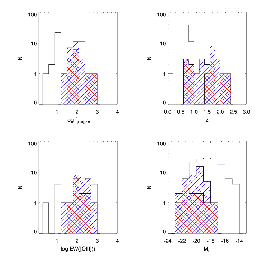
Figure 1: Histogram distributions of the [OIII] line fluxes ($f_{[OIII],-18}=f_{[OIII]}/10^{-18}$erg cm${}^{-2}\;$s^-1), the equivalent width (EW), redshifts, and the absolute B-band magnitude of the 11 ELGs from the combined catalog (red –45 degree tilted line filled) with respect to the Straughn et al. (2009) PEARS ELGs sample (empty black solid line) and the Straughn et al. (2011) WFC3 ERS ELGs sample (blue 45 degree tilted line filled).

The HST/ACS PEARS data reduction was similar to the GRAPES project’s data analysis (Pirzkal et al., 2004), while further steps for identifying emission line sources are described in Meurer et al. (2007) and Straughn et al. (2009). The analysis of the WFC3 ERS data is discussed in Windhorst et al. (2011) and Straughn et al. (2011). The emission line fluxes are measured from 1D extracted spectra, using the IDL code mpfit to fit single or multiple Gaussian line profiles. Due to the marginal splitting of the H$\beta$ and [OIII] doublet, the [OIII] line is fitted with a double Gaussian profile with the ratio of [OIII]$\lambda$4959 to [OIII]$\lambda$5007 constrained to be 1:3 with the same Gaussian widths.

The H$\beta$ line wavelength is fixed at the redshifted wavelength of 4861 Å, given by the observed wavelength of the stronger [OIII]$\lambda$5007 line. The underlying H$\beta$ absorption amounts are obtained by fitting galaxy SEDs (discussed in detail in the next section, Pirzkal et al. 2011) with the population synthesis model of Bruzual & Charlot (2003). The EW of the H$\beta$ absorption features range from 4 – 7 Å, which agrees with the amount obtained in other studies, e.g. $\sim$ 3$\pm$2 Å (Lilly et al., 2003). The absorption feature is smoothed to the same Gaussian profile as the [OIII] line, and then added to the grism spectra. The absorption-corrected H$\beta$ line flux is finally measured by adding a Gaussian profile (same as that of the [OIII] Gaussian profile) with changing amplitude at the fixed wavelength, on the [OIII] already-fitted double Gaussian profiles. An H$\beta$ line flux of S/N$>$3 is assumed as detection, and for line fluxes with S/N$<$3 (1$\sigma\sim 5\times 10^{-18}$erg cm${}^{-2}\;$s^-1), we use a 3$\sigma$ upper limit to the H$\beta$ line flux, which give in a lower limit to the galaxy oxygen abundance on the lower branch (see next section).

The amount of dust extinction is also obtained from the SED fitting, and ranges from $Av=0$–1.2 mag. The extinction correction is done using the IDL code calz$\_$unred (written by W. Landsman), based on the reddening curve from Calzetti et al. (2000). Studies show that the gas can suffer more extinction than the stellar content, hence we assume E(B-V)_stellar=0.44E(B-V)_gas, as has been found locally (Calzetti et al., 2000). Due to the degeneracy of the extinction and the stellar population age, the extinction values have large uncertainties. The uncertainties of the extinction values are folded into the uncertainties in the metallicity. The results show that the uncertainty due to the extinction is in the order of 0.02–0.1 dex, and the dominant part of the uncertainties in the metallicities result from the faint line flux of H$\beta$ compared to [OIII]$\lambda$5007.

Table 1 lists the extinction corrected emission line fluxes and restframe equivalent widths of the [OII]$\lambda$3727, H$\beta$, and the [OIII] doublet for the 11 galaxies in the sample, along with the WFC3 ERS ID and the redshift. Figure 2 shows the grism spectra with the Gaussian fit profiles of the [OII]$\lambda$3727, H$\beta$ and [OIII] doublet lines of the 11 galaxies. Figure 3 shows the GOODS-S $i$-band postage stamps of the 11 galaxies.

To assess the morphologies of the galaxies in our sample, we measure the Gini coefficient $G$, which quantifies the relative distribution of the galaxy’s flux, and the second-order moment of the brightest 20% of the galaxy’s flux (Abraham et al., 2003; Lotz et al., 2004), M₂₀ from the galaxy images. Figure 4 shows the distribution of the galaxies in the G-M₂₀ plane with the empirical line dividing normal galaxies with merger/interacting galaxies (Lotz et al., 2004). The blue stars represent that measured from GOODS $B$-band image and the red triangles show that measured from GOODS $i$-band image. We can see that from the $B$-band image, all of the galaxies lie above the dashed line, which is the region of the outlier galaxies showing merger/interacting and dwarf/irregular morphologies. From the $i$-band image, 8 out of 11 galaxies are on and above the line and 3 are below the line. The visual check of the galaxies below the dashed line shows that two galaxies (246, 578) have obvious multiple knots and irregular shape, and the galaxy 258 is in the region of dwarf galaxies, which is in agreement with the low mass estimation log$(M)=8.74M_{\odot}$. Therefore, we see that 10 out of 11 show disturbing morphologies, interacting companions and tidal features, which demonstrate the ongoing active star-formation in these galaxies. At the same time, the half light radii of the galaxies are shown in Table 2, which span the range from 1 – 8 kpc, with 8 out of 11, $r_{1/2}<$ 3 kpc, showing compact morphology.

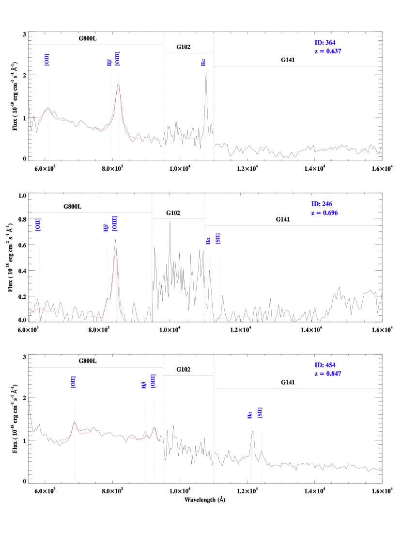
Figure 2: Example of composite grism spectra from the HST/ACS PEARS G800L grism spectroscopy and the HST/WFC3-IR ERS G102 and G141 grism spectroscopy. The emission lines, [OII]$\lambda$3727, H$\beta$, and [OIII]$\lambda$5007, H$\alpha$ and [SII] are detected. The H$\beta$, and [OIII] doublet are detected in both G800L and G102 grisms, and the G102 grism resolves the [OIII]$\lambda\lambda$4959,5007. The fitting of the [OIII] doublet is constrained to make the ratio of the [OIII]$\lambda$4959 to [OIII]$\lambda$5007 fluxes 1:3, and to use the same line width for both. The detection of both [OII] and [OIII] in the composite spectra enables the meatallicity measurement using the R23 method.

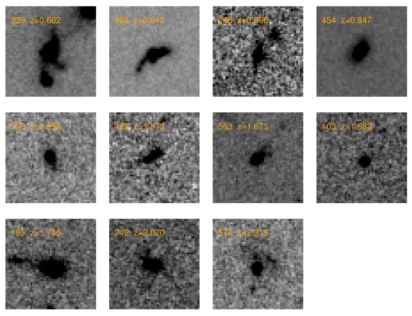
Figure 3: The GOODS-S $i$-band postage stamps of the 11 ERS galaxies in our sample. The irregular morphologies, interacting companions, and tidal features demonstrate ongoing star-formation of these galaxies.

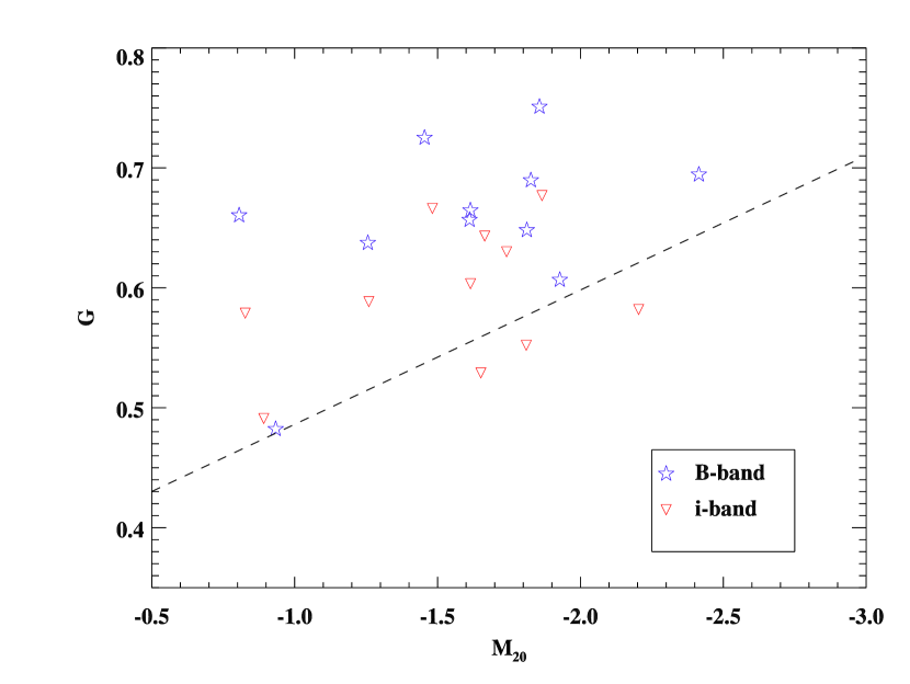
Figure 4: Gini coefficient $G$ vs. M₂₀ to demonstrate the morphology analysis of the 11 galaxies in our sample. The dashed line is the empirical line dividing interacting galaxies (upper region) with normal galaxies (lower region) from Lotz et al. (2004). The blue stars represent galaxies based on $B$-band image analysis. The red triangles are that based on $i$-band image analysis. Most galaxies lie above the line demonstrating disturbed morphologies.

3 Measurements

3.1 Metallicity

Using the strong nebular lines [OII]$\lambda$3727, H$\beta$, and the [OIII] doublet measured from the combined grism spectra, we measure the gas-phase oxygen abundance by the most commonly used $R23$ ($R23$ = ([OII]+[OIII])/H$\beta$) diagnostic indicator (Pagel et al., 1979; Kewley & Dopita, 2002). We calculate the metallicities by iteration, using the parameterized calibrations between the oxygen abundance 12+log(O/H), the ionization parameter $q$, and $R23$ that are derived from theoretical photoionization models by Kewley & Dopita (2002) and Kobulnicky & Kewley (2004).

We select the R23 method, because it relies on measuring some of the brightest nebular emission lines, which allows it to be used for faint galaxies in the distant universe. However, it has one major drawback, which is that the relation between $R_{23}\equiv(f_{OII}+f_{OIII})/f_{H\beta}$ and the gas phase oxygen abundance $12+log(O/H)$ is in general double-valued, with both a high- ($12+log(O/H)>8.5$) and a low- ($12+log(O/H)<8.5$), metallicity branch solution. For the present data set, we rely on a set of three secondary metallicity indicators to decide whether our galaxies lie on the upper or lower branch. First is the “O32” ratio, $f_{OIII}/f_{OII}$. While this is primarily sensitive to the ionization parameter $q$ (Kewley & Dopita, 2002), it can also be used as a branch indicator (Maiolino et al, 2008), with ratios of $f_{OIII}/f_{OII}>2$ indicating a lower branch solution, and $f_{OIII}/f_{OII}<1$ indicating an upper branch solution. Second is the ratio $f_{OIII}/f_{H\beta}$, with $f_{OIII}/f_{H\beta}>3$ indicating $7.4\lesssim 12+log(O/H)\lesssim 8.5$ (Maiolino et al, 2008). Third is the equivalent width of the $H\beta$ line. Hu et al. (2009) show that $\hbox{EW}(H\beta)$ correlates with metallicity, such that $\hbox{EW}(H\beta)\gtrsim 30$Å implies a lower branch solution, and $\hbox{EW}(H\beta)\lesssim 10$Å implies the upper branch solution.

Other popular branch indicators — notably the [OIII]$\lambda$4363 line strength and the $N2$ diagnostic indicator ($N2$ = log ([NII]$\lambda$6584/H$\alpha$) — are not practical for our data set, given the faintness of the [OIII]$\lambda$4363 line, and the blending of [NII]$\lambda$6584 with H$\alpha$ in HST grism spectroscopy. Nevertheless, the combination of $\hbox{EW}(H\beta)$, $f_{OIII}/f_{OII}$, and $f_{OIII}/f_{H\beta}$ provides reasonable confidence in our branch identifications for most of our sample.

Figure 5 shows the $\log(R23)$ versus 12+log(O/H) for our 11 ELGs on the lower branch. The lines represent the model relationships between $\log(R23)$ and 12+log(O/H) at two ionizations with $q=1.0\times 10^{7},1.0\times 10^{8}$. The use of the upper limit of H$\beta$ line fluxes gives the lower limit of R23, and thereafter the lower limit of the metallicities on the lower branch, which are shown as right arrows and upward arrows. Since the galaxies are put on the lower branch, Table 2 shows $\log(R23)$, the ionization parameter $\log(q)$, and the oxygen abundances and their corresponding uncertainties. The large uncertainties on the oxygen abundances are mainly due to the large fractional flux uncertainties for H$\beta$ in our data. All of the galaxies are on the lower branch, and some are near the peak in the $\log(R23)$ vs. metallicity curve, where the branch indicators become both ambiguous and largely irrelevant, and their metallicities are near 12+log(O/H)=8.5.

The galaxy oxygen abundances in our sample span the range from $7.5<12$+log(O/H$)<8.5$, i.e, $\sim$ 0.1 Z$\odot$ – Z$\odot$. (A solar metallicity has Z$\odot$=0.015 and 12+log(O/H) = 8.72, see Allende Prieto et al. 2001). As we see from table 2, the low redshift galaxies at $0.6<z<1$ have an average metallicity of 12+log(O/H)$\simeq$7.95, and the galaxies at $z>1$ have higher average metallicity of 12+log(O/H)$\simeq$8.26, brighter absolute mangitudes and larger stellar masses (see Table 2). This shows the selection effects at low redshift and high redshift of the sample. At same magnitude and line flux limits, the galaxies selected with larger redshifts tend to be more massive, brighter and higher metallicity galaxies. Hence, to evaluate the evolution of the metallicity for same mass galaxies at different redshifts, we need to enlarge the sample to include faint low-mass galaxies at high redshift.

Two galaxies out of the 11 ELGs (ERS ID numbers 339, 364) have followup Magellan spectroscopy, which covers the wavelength range from 4000 to 9000 Å, with a wavelength-resolution of $\sim$ 3 Å (Xia et al., 2012). The metallicities measured from the Magellan spectra using the R23 method on the strong emission lines [OII], H$\beta$ and [OIII] doublet give 12+log(O/H) = 8.07 $\pm$ 0.14 for ERS339 and 8.18 $\pm$ 0.15 for ERS364 (Xia et al., 2012). The metallicities obtained from the HST ACS/WFC3 grism spectra (12+log(O/H) = 8.10${}^{+0.20}_{-0.16}$ for ERS339 and 8.22${}^{+0.16}_{-0.13}$ for ERS364) and that obtained from the Magellan spectroscopic spectra agree to within 1 $\sigma$ ($\sim$ 0.1 dex), underscoring the feasibility of emission-line galaxy metallicity measurements using the HST/WFC3 IR grism data.

Figure 5: The log(R23) versus oxygen abundance for the 11 ELGs in our sample. The overplotted lines represent the theoretical lines at $q=1.0\times 10^{7},1.0\times 10^{8}$ (Kobulnicky & Kewley, 2004). All of the galaxies are put on the lower branch according to the branch criteria. The 3$\sigma$ upper limit of the H$\beta$ line fluxes give the lower limit of log(R23) and hence the lower limit of 12+log(O/H) at the lower branch, which are shown as arrows.

3.2 Stellar Mass

The galaxy stellar masses are derived by comparing the observed photometry with the model spectra library produced by the Bruzual & Charlot (2003) stellar population synthesis code (BC03, hearafter). The galaxies in our sample are located in the ACS pointings of the GOODS-South field. The optical broadband $BViz$ photometry is obtained from HST/ACS GOODS version 2.0 images (Giavalisco et al., 2004). The UV photometry in F225W, F275W, and F336W, as well as the near-IR photometry in F098M (Ys ), F125W (J), and F160W (H) are from the new WFC3 ERS mosaics (Windhorst et al., 2011). In this paper, we adopt the galaxy stellar masses measured by the method of Bayesian based Markov Chain Monte Carlo ($\pi$MC²), which allows us to compare the observations to arbitrarily complex models, and to compute 95% credible intervals that provide robust constraints for the model parameter (see Pirzkal et al. 2011 for details). The models are generated using the single (SSP), two (SSP2) stellar instantaneous populations, or an exponentially decaying star formation history model (EXP). The parameters assumed in the models are Salpeter initial mass function (IMF), metallicities ranging from $Z=0.004$ to 0.02 (Z_⊙), the stellar population ages, the relative ratio between the old and young stellar populations, the Calzetti et al. (2000) extinction law, and the half-life $\tau$ value in the case of EXP models. We divide by a factor of 1.8 to make the galaxy stellar masses derived from Salpeter IMF in this paper consistent with that in other studies derived from Chabrier (2003) IMF (Erb et al., 2006). The comparison of the R23 and the SED best-fit metallicities shows agreement to within $\sim$ 0.1 dex for 6 galaxies, and $\sim$ 0.5 dex higher metallicity for the other 5 galaxies from the SED fitting method. The higher metallicity has very little effect on the estimated galaxy masses as shown by Pirzkal et al. (2011). The results of the galaxy stellar masses and stellar population ages are shown in the sixth column of Table 2. The galaxies show young ages of 20–90 Myr and low masses $\sim$ $10^{8}-10^{10}M_{\odot}$.

4 Results

The wide spectral coverage of the HST/ACS PEARS and WFC3 ERS composite grism spectra provide galaxies at $0.6<z<2.4$ with full set of emission lines [OII], H$\beta$ and [OIII], which extend the study of the evolution of the L-Z relation and the M-Z relation to redshift $z\simeq$ 2.5. In this section, we will show the results of the luminosity-metallicity relation and the mass-metallicity relation, which provide important clues to the evolution of galaxies by comparing with the relations at different redshifts.

4.1 L-Z relation

Previous results show important evolution of the slope and the zero point of the L-Z relation with respect to redshift, decreasing metallicity with increasing redshift at a given luminosity. With the sample of 11 grism ELGs at $0.6<z<2.4$, we investigate the evolution of the L-Z relation with redshift. Following traditions, we present the rest-frame absolute $B$-band magnitude as a measure of the luminosities. The restframe $B$-band absolute magnitudes are computed from the best-fit SED with the BC03 stellar population synthesis model.

Figure 6 shows the relationship between the absolute rest-frame $B$ magnitude versus the gas-phase oxygen abundance derived from $R23$ diagnostic indicator. The lines plotted in Figure 6 are the local L-Z relation obtained by Tremonti et al. (2004) for $\sim$53,000 SDSS galaxies at $z\sim 0.1$ (solid line), the L-Z relation obtained by Zahid et al. (2011) from 1350 DEEP2 emission line galaxies at z $\sim$ 0.8 (dashed line), that obtained by Hu et al. (2009) from a sample of Ultra-Strong Emission-Line (USELs) galaxies at $z\simeq$0–1 (dotted line and empty stars), and that of Salzer et al. (2009) for 15 star-forming galaxies at $z\sim 0.3$ (open upside down triangles). Our sample of 11 galaxies span a range in luminosity –17 $<M_{B}<$ –23 and in metallicity $7.5<12$+log(O/H$)<8.5$. The red solid dots represent the galaxies with $z>1$, and the green triangles represent the galaxies with $z<1$. The blue solid line shows the best linear fit of the 11 galaxies, a relation of 12+log(O/H$)=(4.75\pm 0.86)-(0.17\pm 0.04)M_{B}$ with a correlation coefficience of –0.77.

Compared to the other relationships shown in Figure 6, ACS+WFC3 grism galaxies are about 7 magnitudes brighter in luminosities than the local SDSS galaxies and the $z\sim$ 0.8 DEEP2 galaxies at fixed metallicity. The DEEP2 sample (Zahid et al., 2011) shows little evolution compared to the SDSS sample, about $\sim$ 0.1 dex relative to the local L-Z relation, while the ERS grism galaxies show $\sim$ 0.6 dex lower metallicities than the SDSS galaxies at given luminosity. The grism galaxies show a good match with metal-poor galaxies of Hu et al. (2009); Salzer et al. (2009) along the fitted L-Z relation.

The Hu et al. (2009) USELS galaxies have high equivalent width with EW(H$\beta>30$Å), extend to fainter galaxies to M${}_{B}\sim$ –16 and show low metallicities of $7.1<12$+log(O/H$)<8.4$. The Salzer et al. (2009) are [OIII]-selected galaxies ([OIII]/H$\beta>$3) at $z\sim$0.3 and show brighter luminosity and higher metallicities. The difference of the galaxies on the L-Z figure shows the different physical properties of the three samples: the USELS are basically selected to be fainter dwarf galaxies, the low redshift Salzer et al. (2009) are [OIII]-selected brighter galaxies. Since the three samples follow well of the L-Z relationship of the metal-poor galaxies, and the L-Z relations of the SDSS galaxies and the DEEP2 galaxies are obtained by averaging large samples, we conclude that the big offset in the L-Z relation between the local and the three metal-poor galaxies samples is due to the selection of a sample of young strong emission-line star-forming galaxies, which will be further illustrated in the next subsection.

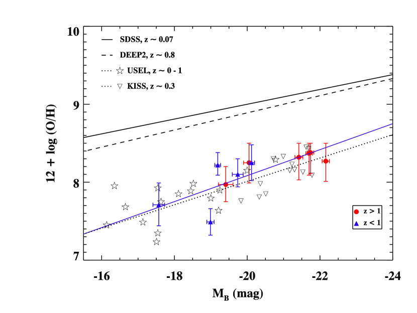
Figure 6: $L$-$Z$ relation between the rest-frame $B$-band absolute magnitude versus the oxygen abundance for the 10 emission line galaxies at $0.6<z<2.4$. The metallicity is derived from the $R23$ indicator and the $x$-axis is the rest-frame $B$-band absolute magnitude. The red solid dots represent the galaxies with $z>1$, and the blue triangles represent the galaxies with $z<1$. The solid line represents the relation obtained by Tremonti et al. (2004) for SDSS star-forming galaxies at $z\sim 0.1$. The dashed line illustrates the relation obtained by Zahid et al. (2011) for DEEP2 galaxies at $z\sim 0.8$. The dotted line and the empty stars show the relation obtained by Hu et al. (2009) for USEL galaxies at $z=0-1$. The empty upside down triangles are that of Salzer et al. (2009) for [OIII]-selected $z\sim 0.3$ galaxies. The blue solid line shows the best linear fit of our sample, which gives a relationship of $12+$log$(O/H)=(4.75\pm 0.86)-(0.17\pm 0.04)M_{B}$. The PEARS sample shows an offset by about –0.6 dex in metallicity relative to the local relation at $z\sim 0.1$.

4.2 M-Z relation

Figure 7 shows the relation between the stellar masses and the gas-phase oxygen abundances for the 11 star-forming galaxies in our sample at $0.6<z<2.4$. The solid line represents the $M$-$Z$ relation at $z\sim 0.1$ from Tremonti et al. (2004) for the local SDSS galaxies, which are selected to be star-forming galaxies based on lines H$\alpha$, H$\beta$, and [NII]. The dashed line shows the $M$-$Z$ relation at $z\sim 0.8$ for the 1350 H$\beta$ selected blue DEEP2 galaxies from Zahid et al. (2011). The dotted line and the dash-dotted line are UV-color selected galaxies at $z\sim 2.3$ from Erb et al. (2006) and the UV-selected Lyman Break Galaxies (LBGs) at $z\sim 3.1$ from Mannucci et al. (2009), respectively. The red line shows the best fit to the M-Z relation for the ELGs in our sample.

The green triangles illustrate the sample of the “green peas” from Cardamone et al. (2009) and Amorin et al. (2010), which are extremely compact (r$<3$ kpc) star-forming galaxies at $0.11<z<0.35$ selected by color from the SDSS spectroscopic observation, with an unsual large equivalent width of up to $\sim$ 1000 Å. We recalculate the gas-phase oxygen metallicity by the R23 method for the “green peas” sample. Also plotted are the Ly$\alpha$ emitters at $z\sim 0.3$, and $\sim$2.3 from Finkelstein et al. (2011a,b), shown in empty red circles and black asterisks with 2 $\sigma$ and 3 $\sigma$ upper limits, and one extremely metal poor galaxies XMPG WISP5-230 (Atek et al., 2011). All data presented have been scaled to a Chabrier (2003) IMF. To ensure the consistency of the comparison, the conversion given by Kewley & Ellison (2008) is used to convert to the same metallicity calibration of Kobulnicky & Kewley (2004) to avoid the differences arising from different metallicity indicators (Zahid et al., 2011). The metallicity of the XMPG galaxy from Atek et al. (2011) is measured by the direct $Te$ method, and is not converted to the same metallicity diagnostic due to the absence of the [OII] flux and the conversion relationship between the direct $Te$ method and the R23 method in Kobulnicky & Kewley (2004).

From Figure 7, our grism galaxies span the range $8.1<$log$(M_{*}/$M${}_{\odot})<10.1$ and $7.5<12$+log(O/H$)<8.5$, with the average values of $<$log(M${}_{*}/M_{\odot})>=9.3$ and $<$12+log(O/H)$>=8.1$. Although this is a small sample, it shows a similar correlation between metallicity and stellar mass, increasing oxygen abundance with the increase of the stellar masses. The red dots in Figure 7 show the 6 galaxies with redshift $z>1$ and with emission lines observed in WFC3 ERS. The blue triangles represent the galaxies with $0.6<z<1$. We fit the mass-metallicity relation with a second-order polynomial (Maiolino et al, 2008):

$$12+log(O/H)=A[log(M)-log(M_{0})]^{2}+K_{0},$$ (1)

the best fit parameters to the 11 ELGs in our sample give A=-0.07, log(M₀)=11.87, K₀=8.63. From Table 2, we see that these high redshift galaxies have higher stellar masses with a mean of $<logM_{*}/$M${}_{\odot}>\simeq$ 9.6 and higher metallicities with a mean of $<$12+log(O/H)$>$$\simeq$ 8.3. The low redshift subsample have lower galaxy stellar masses with a mean of $<$log$M_{*}/$M_⊙$>$$\simeq$ 8.8 and lower metallicities with a mean of $<$12+log(O/H)$>$$\simeq$ 8.0. The offset shown between the high redshift subsample and the low redshfit subsample includes the evolution of the M-Z relation with redshift, and the selection effect, that for the same emission line detection the high redshift galaxies tend to be more luminous, more massive and more metal-enriched than the low redshift galaxies.

We examine the M-Z relation by comparing our sample with that at different redshift ranges. Compared with the local relation at $z\sim 0.1$, the SDSS galaxies with comparable stellar mass to the average of the grism sample, $M_{*}\sim 10^{9.3}$ M_⊙, have $12+$log$(O/H)\simeq$ 8.8, which is about $\sim$ 0.6 dex higher than the average of the grism galaxies. For the low redshift subsample with a mean of $z\simeq 0.8$, the M-Z relation show a large offset of $\sim$ 0.6 dex with that of Zahid et al. (2011) at $z\simeq 0.8$ too. This big difference between our sample and that of Tremonti et al. (2004) and Zahid et al. (2011) is mainly due to the different selection criteria of the galaxies. The local SDSS galaxies (Tremonti et al., 2004) and the DEEP2 galaxies (Zahid et al., 2011) are obtained from large spectroscopic survey, and the M-Z relations show the average relationships of the dominant galaxy populations at that redshift. Table 3 lists the physical properties including redshift range, selection, absolute magnitude, emission line EW, half light radius and SFR of the different comparing samples. We can see that the SDSS and DEEP2 samples are not selecting high EW star-forming galaxies compared with the “green peas” (Amorin et al., 2010), USELS (Hu et al., 2009), LBGs (Mannucci et al., 2009) and our PEARS/ERS ELGs, which are biased to high EW emission-lines (up to $\sim$ 1000 Å) and compact ($r_{1/2}<3$ kpc) galaxies.

For the high-redshift subsample with a mean of $z\simeq 2$, the M-Z relation shows an offset of $\sim$ 0.2 dex with respect to that of the LBGs at $z\simeq 2.3$ (Erb et al., 2006). The low metallicity galaxies basically fall between the relation at $z\simeq 2.3$ and $z\simeq 3.1$ and have low metallicities down to 12+log(O/H)$\sim$7.5, 7.7. The “green peas” (Hoopes et al., 2007; Overzier et al., 2008; Amorin et al., 2010) at $z\simeq 0.3$ are found to be metal-poor by $\sim$ 0.5 dex relative to other galaxies of similar stellar mass, and show compact and distrubed morphology. From Figure 7, we find that 7 out of 11 of the HST/ACS+WFC3 grism emission line galaxies are in the similar metallicity range 12+log(O/H)$\sim$8.3 and four galaxies are more metal-poor by up to 0.6 dex, compared with the green peas at the same galaxy stellar masses, which shows significant chemical enrichment from $z\simeq 0.8$ to $z\simeq 0.3$ at the low stellar mass range. To confirm this evolution with higher statistical significance, we will need larger sample of galaxies extending to low mass faint galaxies at high redshifts. The strong emission line selected Ly$\alpha$ galaxies at $z\simeq 0.3$, at $z\simeq 2.3$ and XMPG WISP5$\_$230 at $z\simeq 0.7$ show similar lower metallicities at $7.2<12+log(O/H)<8.2$ with respect to the average M-Z relations obtained from large survey samples.

The detailed analysis of the morphologies, sizes, colors, SSFRs based on the M-Z relation (Pirzkal et al., 2006; Xia et al., 2012) show that the strong emission-line selected grism galaxies are biased towards young compact interacting dwarf star-forming galaxies. Pirzkal et al. (2006) shows small physical sizes of $\sim$ 1–2 kpc for the emission line galaxies observed from the GRAPES survey, and Xia et al. (2012) presents high SSFRs $10^{-9}-10^{-7}/yr$ for the ELGs from the PEARS survey. Since the galaxies in our sample are partly the subsample of the PEARS ELGs, the results of the sizes and the SSFRs are consistent with the previous results, with $r_{1/2}<3kpc$ and $SSFR\sim 10^{-9}/yr$. This confirms the selection effects of the young compact disturbed emission line galaxies in the sample. The early stage of galaxy evolution (downsizing effect) or interaction-induced pristine gas inflow picture may account for the offset of the grism galaxies in metallicity relative to the local sample.

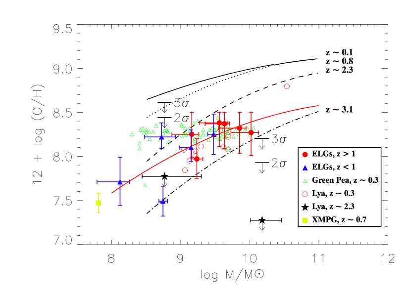
Figure 7: Relation between the stellar masses and the gas-phase oxygen abundances for our sample of 11 ELGs from PEARS and ERS grism data at $0.6<z<2.4$. The metallicities are estimated from the $R23$ method. The stellar masses are estimated from the SED fitting with $BC03$ model and have been scaled to a Chabrier (2003) IMF to be consistent with other studies. The definition of the points of our sample are the same as Figure 5. Also plotted for comparison are the green peas (empty green triangulars) at z$\simeq$0.3 (Amorin et al., 2010), Ly$\alpha$ galaxies at $z\simeq 0.3$ and $z\simeq 2.3$ (Finkelstein et al., 2011a, b), and the WISP XMPG galaxy at $z\simeq 0.7$ (Atek et al., 2011). The solid red line is the best fit of the M-Z relation to the 11 ELGs in our sample. The solid line represents the M-Z relation at $z\simeq 0.1$ from Tremonti et al. (2004) for the local SDSS galaxies. The dashed line shows the M-Z relation at $z\simeq 0.8$ for the 1350 DEEP2 galaxies from Zahid et al. (2011). The dotted line and the dash-dotted line are that at $z\simeq 2.3$ from Erb et al. (2006) and at $z\simeq 3.1$ from Mannucci et al. (2009), respectively. The M-Z relations at different redshifts are calibrated to the same metallicity indicator of Kobulnicky & Kewley (2004) from Zahid et al. (2011). The large offset of $\sim$ 0.5 dex of this sample relative to the other relations at similar redshift demonstrates that these galaxies may be at the early-stages of galaxy evolution. Infall of gas due to mergers is another popular explanation, e.g. Peeples et al. (2009).

5 Discussion and Summary

We use a sample of 11 emission line galaxies at $0.6<z<2.4$ observed by HST/ACS PEARS and HST WFC3 ERS programs at 0.6–1.6 $\mu$m to demonstrate the effectiveness of the grism spectra (R $\sim$ 100–300) used for the metallicity measurement. With the [OII], H$\beta$, and [OIII] lines in the composite spectra of the two grism spectra surveys, we use the $R23$ method to derive the gas-phase oxygen abundances, 12+log(O/H). For two galaxies which have the follow-up Magellan spectroscopy, the metallicities obtained from the grism spectra and from the Magellan spectroscopic spectra are consistent to within 1 $\sigma$ (0.1 dex), which demonstrates the feasibility of the HST/WFC3 IR grism spectra used here for the study of galaxy metallicities.

The measured gas-phase abundances are in the low metallicity range $7.5<12$+log(O/H$)<8.5$. The galaxy stellar masses are derived from MCMC SED fitting and span the range 8.1 $<$ log($M_{*}/$M_⊙) $<$ 10.1. Both the L-Z relation and the M-Z relation show that with the increase of the galaxy stellar mass or the luminosity, the metallicity increases, which agrees with the enrichment history of galaxy evolution. The M-Z relation of this sample show significant offset by about –0.6 dex in metallicity at given stellar mass relative to the local M-Z relation from SDSS galaxies and the galaxies from the DEEP2 survey at similar redshifts $z\simeq 0.8$. The L-Z relation is fitted by a straight line of 12+log(O/H$)=(4.75\pm 0.86)-(0.17\pm 0.04)M_{B}$ with a correlation coefficience of –0.77, which is also offset by about –0.6 dex in metallicity relative to the local and $z\simeq 0.8$ L-Z relations.

Our sample of galaxies at $z\simeq 0.8$ show similarity to the local green peas in morphology and low metallicity. Two galaxies show significant poorer metallicity by $\sim$0.5 dex compared with the “green peas” at the same galaxy stellar masses, which signifies different physical processes in the galaxy evolution and chemical enrichment from $z\simeq 0.8$ to $z\simeq 0.2$ at the low stellar mass range. The different contribution by downsizing and gas inflow/outflow need to be examined in detail by larger samples further.

By comparing the PEARS/ERS sample with other emission-line selected samples (Erb et al., 2006; Hu et al., 2009; Mannucci et al., 2009; Salzer et al., 2009; Amorin et al., 2010; Zahid et al., 2011; Finkelstein et al., 2011a, b) in Table 3, we find that the physical properties of the ELGs galaxies at different redshifts show great similarities: e.g. (1) ultra-strong emission lines of about $10^{-17}$erg cm${}^{-2}\;$s^-1, high emission-line EWs up to $\sim$ 1000 Å, and hence very high SSFRs to $10^{-9}/yr$; (2) compact morphology ($r_{1/2}<3kpc$); (3) evidence for mergers/interactions from the asymmetries of the morphology, such as companions and wispy tidal tails around a compact star-forming region, three “green peas” shown in Cardomone et al. (2009), and 10 out of 11 galaxies in our sample (see Figure 3). Hence, we conclude that the offsets shown in the M-Z and L-Z relations with respect to that obtained from average of large sample are mainly due to the selection effects based on prominent emission lines. van der Wel et al. (2011) shows an abundant population of extreme emission line galaxies (EELGs) from the HST/WFC3 CANDELS Survey (Cosmic Assembly Near-IR Deep Extragalactic Legacy Survey) and confirms the physical properties of low stellar masses $\sim$ 10${}^{8}M_{\odot}$, and strong outflows due to enormous starbursts in the EELGs by the HST/WFC3 grism spectra.

Taken together, the properties of the ELGs: compact starbursts, low metallicities, disturbed morphologies, and low masses, indicate that these are dwarf galaxies undergoing their early stages of galaxy evolution with prominent signs of strong activities of interaction (gas accretion and outflow) with companion galaxies. Both the downsizing effect and inflow/outflow play important roles in these low metallicity galaxies’ evolution. To examine the mode of the star-formation of these low-mass, low-metallicity galaxies in the whole scenario of galaxy evolution requires a larger sample of this kind of ELGs from optical to NIR spectroscopy with morphologies to give us a more comprehensive picture of these galaxies. Trump et al. (2011) presents a sample of 28 emission line galaxies at $z\sim 2$ with prominent [OIII] and H$\beta$ in the GOODS-S region of the Cosmic Assembly Near-infrared Deep Extra-galactic Legacy Survey(CANDELS). Combined with the PEARS spectra, this sample will greatly enhance the sample at redshift $z~{}2$ at the low-mass low-metallicity region of the M-Z relation, which is important to study and understand the physical processes effecting galaxy evolution.

Table 1: The extinction corrected emission line fluxes and equivalent widths of the PEARS/ERS grism galaxies. The H$\beta$ line fluxes are absorption corrected by the SED fitting. The detections of the H$\beta$ line are set with S/N$>$3. The 3$\sigma$ upper limit of the H$\beta$ line is used for galaxies with S/N$<$3. These galaxies are marked with stars.

ID	$z$	R.A.	DEC.	E(B-V)	[OII]3727	EW([OII])	H$\beta$	EW(H$\beta$)	[OIII]	EW([OIII])
		(deg)	(deg)	(mag)	($10^{-18}$erg s${}^{-1}\;$cm-2)	(Å)	($10^{-18}$erg s${}^{-1}\;$cm-2)	(Å)	($10^{-18}$erg s${}^{-1}\;$cm-2)	(Å)
339	0.602	53.0773392	-27.7081985	0.30${}^{+0.30}_{-0.30}$	645.51 $\pm$ 162.65	29	468.41 $\pm$ 45.19	61	2373.95 $\pm$ 56.24	334
364	0.642	53.0693359	-27.7090893	0.03${}^{+0.18}_{-0.03}$	80.90 $\pm$ 15.93	40	50.35 $\pm$ 7.24	38	308.61 $\pm$ 9.59	248
246	0.696	53.0700035	-27.7165890	0.03${}^{+0.16}_{-0.03}$	4.50 $\pm$ 4.50	26	22.90 $\pm$ 5.22	352	121.91 $\pm$ 6.92	1605
454	0.847	53.0761719	-27.7011452	0.16${}^{+0.09}_{-0.10}$	166.57 $\pm$ 17.80	28	45.22 $\pm$ 13.92	11	86.35 $\pm$ 18.02	22
258	0.998	53.0857124	-27.7113400	0.03${}^{+0.06}_{-0.03}$	29.98 $\pm$ 4.25	74	73.63 $\pm$ 35.74 ⋆	525	241.91 $\pm$ 47.48	729
432	1.573	53.0484200	-27.7095337	0.08${}^{+0.16}_{-0.08}$	101.97 $\pm$ 23.19	44	24.21 $\pm$ 11.76 ⋆	16	132.11 $\pm$ 15.56	108
563	1.673	53.0705452	-27.6956444	0.14${}^{+0.20}_{-0.14}$	93.91 $\pm$ 17.34	46	13.95 $\pm$ 9.06 ⋆	19	122.04 $\pm$ 11.86	165
103	1.682	53.0633392	-27.7272835	0.06${}^{+0.13}_{-0.06}$	43.55 $\pm$ 10.23	93	9.84 $\pm$ 7.81 ⋆	45	52.83 $\pm$ 10.33	193
195	1.745	53.0656700	-27.7203941	0.09${}^{+0.09}_{-0.09}$	87.84 $\pm$ 13.89	37	21.25 $\pm$ 8.28 ⋆	17	109.87 $\pm$ 10.91	94
242	2.070	53.0821304	-27.7137547	0.19${}^{+0.17}_{-0.17}$	94.79 $\pm$ 29.03	72	13.39 $\pm$ 8.57 ⋆	25	79.46 $\pm$ 11.19	143
578	2.315	53.0589218	-27.6978111	0.26${}^{+0.11}_{-0.19}$	116.58 $\pm$ 21.06	98	12.29 $\pm$ 10.42 ⋆	10	65.98 $\pm$ 13.53	35

Table 2: The ionization parameter, metallicity, half-light radius, absolute magnitude, galaxy stellar mass and SFR, SSFR of the PEARS/ERS grism galaxies. The missing upper errors in log$R23$ and 12+log(O/H) denote the lower limits due to the use of the upper limits of H$\beta$ line fluxes. The galaxy stellar masses derived from Salpeter IMF are scaled to that from Chabrier (2003) IMF to be consistent in comparison with other studies.

ID	$z$	log($R23)$	log $q$	12+log(O/H)	$r_{1/2}$	$M_{B}$	log $M_{*}$	Age	SFR	SSFR
(1)	(2)	(3)	(4)	(5)	(kpc)	(mag)	($M_{\odot}$)	(Myr)	($M_{\odot}$/yr)	($\times 10^{-9}$/yr)
339	0.604	0.81${}^{+0.05}_{-0.05}$	8.12 $\pm$ 1.28	8.10${}^{+0.20}_{-0.16}$	8.10	–19.74	9.19 ${}^{+0.02}_{-0.34}$	—	15.20 $\pm$ 1.72	10.64 $\pm$ 4.16
364	0.637	0.89${}^{+0.07}_{-0.07}$	7.97 $\pm$ 0.10	8.22${}^{+0.16}_{-0.13}$	1.72	–19.19	8.72 ${}^{+0.21}_{-0.25}$	56.9${}_{-53.7}^{+27.7}$	1.70 $\pm$ 0.39	1.90 $\pm$ 0.84
246	0.691	0.74${}^{+0.10}_{-0.10}$	8.58 $\pm$ 0.51	7.71${}^{+0.28}_{-0.27}$	1.97	–17.57	8.12 ${}^{+0.14}_{-0.33}$	50.4${}_{-47.1}^{+0.04}$	1.06 $\pm$ 0.21	3.31 $\pm$ 0.81
454	0.847	0.75${}^{+0.14}_{-0.14}$	7.29 $\pm$ 0.17	8.25${}^{+0.23}_{-0.23}$	1.37	–20.12	9.48 ${}^{+0.08}_{-0.08}$	60.8${}_{-32.1}^{+71.5}$	2.41 $\pm$ 1.40	0.60 $\pm$ 0.37
258	0.997	0.40${}^{+}_{-0.16}$	8.02 $\pm$ 0.11	7.49${}^{+}_{-0.17}$	2.20	–18.99	8.74 ${}^{+0.06}_{-0.06}$	90.1${}_{-35.3}^{+35.8}$	5.78 $\pm$ 3.66	7.83 $\pm$ 5.61
432	1.573	0.82${}^{+}_{-0.15}$	7.58 $\pm$ 0.13	8.25${}^{+}_{-0.26}$	4.14	–20.05	9.16 ${}^{+0.10}_{-0.29}$	51.0${}_{-47.8}^{+44.5}$	2.71 $\pm$ 2.44	1.73 $\pm$ 1.56
563	1.673	0.90${}^{+}_{-0.15}$	7.64 $\pm$ 0.13	8.37${}^{+}_{-0.28}$	1.58	–21.70	9.63 ${}^{+0.07}_{-0.28}$	46.5${}_{-43.3}^{+52.2}$	3.66 $\pm$ 2.24	0.51 $\pm$ 0.37
103	1.682	0.61${}^{+}_{-0.16}$	7.46 $\pm$ 0.12	7.97${}^{+}_{-0.22}$	1.07	–19.41	9.23 ${}^{+0.08}_{-0.07}$	93.1${}_{-68.8}^{+72.8}$	1.59 $\pm$ 1.35	0.88 $\pm$ 0.83
195	1.745	0.90${}^{+}_{-0.15}$	7.61 $\pm$ 0.10	8.38${}^{+}_{-0.27}$	1.89	–21.74	9.56 ${}^{+0.13}_{-0.29}$	23.9${}_{-20.8}^{+29.2}$	3.80 $\pm$ 2.02	2.30 $\pm$ 1.22
242	2.070	0.83${}^{+}_{-0.16}$	7.46 $\pm$ 0.21	8.32${}^{+}_{-0.29}$	2.09	–21.42	9.85 ${}^{+0.09}_{-0.30}$	39.7${}_{-36.5}^{+55.1}$	14.51 $\pm$ 9.60	1.91 $\pm$ 1.37
578	2.315	0.77${}^{+}_{-0.16}$	7.32 $\pm$ 0.16	8.27${}^{+}_{-0.26}$	5.82	–22.16	10.02 ${}^{+0.11}_{-0.29}$	19.0${}_{-15.8}^{+40.2}$	19.17 $\pm$ 12.81	0.50 $\pm$ 0.53

Table 3: The selection criteria and physical properties of the comparison samples in the paper.

Sample	Survey	$z$	Selection	$f_{line}$	$M_{B}$	EW	r1/2	SFR
(1)	(2)	(3)	(4)	($10^{-17}$erg cm${}^{-2}\;$s-1)	(mag)	(Å)	(kpc)	(M⊙/yr)
Tremonti et al. (2004);	SDSS	0.005$<z<$0.25	H$\alpha$, H$\beta$, [NII]	—	(-16, -22)	EW(H$\alpha)\sim$3-200	–	–
Salzer et al.(2009);	KISS	$z\sim$0.3	[OIII]	—	(-19.5, -22.5)	—	–	–
Finkelstein et al. (2011b); LAEs	HETDEX	$z\sim$0.3	Ly$\alpha$	$>$ 1400	—	EW([Ly$\alpha$]) $\sim$ 20-40	–	–
Amorin et al. (2010); green pea	SDSS	0.11$<z<$0.35	color	—	—	EW([OIII]) $<$ 1000	$<$ 3	$<$ 30
Zahid et al. (2011)	DEEP2	0.75$<z<$0.82	H$\beta$, color	—	(-19.5, -22)	$<$EW(H$\beta)>\sim$8.9	–	–
Hu et al. (2009); USELS	DEMOS	0$<z<$1	[OIII], H$\alpha$	$>$ 1.5	(-16, -21)	EW(H$\beta)<$ 500	–	–
Erb et al. (2006);	LRIS-B	$z\sim$2.3	UV-colors	$>$ 15	(-20.5, -23.5)	—	–	20 – 60
Finkelstein et al. (2011a); LAEs	HETDEX	$z\sim$2.3	Ly$\alpha$	$>$ 200	—	EW([OIII]) $<$ 300	–	20 – 40
Mannucci et al. (2009); LBGs	AMAZE, LSD	2.6$<z<$3.4	—	$>$ 1.1	—	—	0.7 – 2.4	5 – 40
This paper	PEARS, ERS	0.6$<z<$2.3	Emission lines	$>$ 5	(-17.5, -22.5)	EW([OIII]) $<$ 1600	1 – 8.1	1 – 20

References

- Abraham et al. (2003) Abraham, R., van den Bergh, S., & Nair, P. 2003, ApJ, 588, 218
- Allende Prieto et al. (2001) Allende Prieto, C. A., Lambert, D. L., & Asplund, M. 2001, ApJ, 556, L63
- Amorin et al. (2010) Amorin, R. O., Enrique, P. M., & Vilchez, J. M. 2010, ApJ, 715, 128
- Atek et al. (2011) Atek, H., et al. 2011, ApJ, 743, 121
- Bruzual & Charlot (2003) Bruzual, G., & Charlot, S. 2003, ApJ, 405, 538
- Cardamone et al. (2009) Cardamone, C., et al. 2009,
- Calzetti et al. (2000) Calzetti, D., et al. 2000, ApJ, 533, 682
- Erb et al. (2006) Erb, D. K., Shapley, A. E., Pettini, M., et al. 2006, ApJ, 644, 813