Multi-Adaptive Galerkin Methods for ODEs II:
implementation and Applications

Abstract

Continuing the discussion of the multi-adaptive Galerkin methods $\mathrm{mcG}(q)$ and $\mathrm{mdG}(q)$ presented in [A. Logg, SIAM J. Sci. Comput., 24 (2003), pp. 1879–1902], we present adaptive algorithms for global error control, iterative solution methods for the discrete equations, features of the implementation Tanganyika, and computational results for a variety of ODEs. Examples include the Lorenz system, the solar system, and a number of time-dependent PDEs.

sisc20032541119–1141

1 Introduction

In this paper we apply the multi-adaptive Galerkin methods $\mathrm{mcG}(q)$ and $\mathrm{mdG}(q)$, presented in [10], to a variety of problems chosen to illustrate the potential of multi-adaptivity. Throughout this paper, we solve the ODE initial value problem

(1) $$\left\{\begin{array}[]{rcl}\dot{u}(t)&=&f(u(t),t),\ t\in(0,T],\\ u(0)&=&u_{0},\end{array}\right.$$

where $u:[0,T]\rightarrow\mathbb{R}^{N}$, $f:\mathbb{R}^{N}\times(0,T]\rightarrow\mathbb{R}^{N}$ is a given bounded function that is Lipschitz continuous in $u$, $u_{0}\in\mathbb{R}^{N}$ is a given initial condition, and $T>0$ a given final time.

We refer to [10] for a detailed description of the multi-adaptive methods. Here we recall that each component $U_{i}(t)$ of the approximate solution $U(t)$ is a piecewise polynomial of degree $q_{i}=q_{i}(t)$ on a partition of $(0,T]$ into $M_{i}$ subintervals of lengths $k_{ij}=t_{ij}-t_{i,j-1}$, $j=1,\ldots,M_{i}$. On the interval $I_{ij}=(t_{i,j-1},t_{ij}]$, component $U_{i}(t)$ is thus a polynomial of degree $q_{ij}$.

Before presenting the examples, we discuss adaptive algorithms for global error control and iterative solution methods for the discrete equations. We also give a short description of the implementation Tanganyika.

2 Adaptivity

In this section we describe how to use the a posteriori error estimates presented in [10] in an adaptive algorithm.

2.1 A strategy for adaptive error control

The goal of the algorithm is to produce an approximate solution $U(t)$ to (1) within a given tolerance $\mathrm{TOL}$ for the error $e(t)=U(t)-u(t)$ in a given norm $\|\cdot\|$. The adaptive algorithm is based on the a posteriori error estimates, presented in [10], of the form

(2) $$\|e\|\leq\sum_{i=1}^{N}\sum_{j=1}^{M_{i}}k_{ij}^{p_{ij}+1}r_{ij}s_{ij}$$

or

(3) $$\|e\|\leq\sum_{i=1}^{N}S_{i}\max_{j}k_{ij}^{p_{ij}}r_{ij},$$

where $\{s_{ij}\}$ are stability weights, $\{S_{i}\}$ are stability factors (including interpolation constants), $r_{ij}$ is a local measure of the residual $R_{i}(U,\cdot)=\dot{U}_{i}-f(U,\cdot)$ of the approximate solution $U(t)$, and where we have $p_{ij}=q_{ij}$ for $\mathrm{mcG}(q)$ and $p_{ij}=q_{ij}+1$ for $\mathrm{mdG}(q)$.

We use (3) to determine the individual time-steps, which should then be chosen as

(4) $$k_{ij}=\left(\frac{\mathrm{TOL}/N}{S_{i}\ r_{ij}}\right)^{1/{p_{ij}}}.$$

We use (2) to evaluate the resulting error at the end of the computation, noting that (2) is sharper than (3).

The adaptive algorithm may then be expressed as follows: Given a tolerance $\mathrm{TOL}>0$, make a preliminary guess for the stability factors and then

1. solve the primal problem with time-steps based on (4).

2. solve the dual problem and compute stability factors and stability weights.

3. compute an error estimate $E$ based on (2).

4. if $E\leq\mathrm{TOL}$, then stop, and if not, go back to (i).

Although this seems simple enough, there are some difficulties involved. For one thing, choosing the time-steps based on (4) may be difficult, since the residual depends implicitly on the time-step. Furthermore, we have to choose the proper data for the dual problem to obtain a meaningful error estimate. We now discuss these issues.

2.2 Regulating the time-step

To avoid the implicit dependence on $k_{ij}$ for $r_{ij}$ in (4), we may try replacing (4) with

(5) $$k_{ij}=\left(\frac{\mathrm{TOL}/N}{S_{i}\ r_{i,j-1}}\right)^{1/{p_{ij}}}.$$

Following this strategy, if the time-step on an interval is small (and thus also is the residual), the time-step for the next interval will be large, so that (5) introduces unwanted oscillations in the size of the time-step. We therefore try to be a bit more conservative when choosing the time-step to obtain a smoother time-step sequence. For (5) to work, the time-steps on adjacent intervals need to be approximately the same, and so we may think of choosing the new time-step as the (geometric) mean value of the previous time-step and the time-step given by (5). This works surprisingly well for many problems, meaning that the resulting time-step sequences are comparable to what can be obtained with more advanced regulators.

We have also used standard PID (or just PI) regulators from control theory with the goal of satisfying

(6) $$S_{i}k_{ij}^{p_{ij}}r_{ij}=\mathrm{TOL}/N,$$

or, taking the logarithm with $C_{i}=\log(\mathrm{TOL}/(NS_{i}))$,

(7) $$p_{ij}\log k_{ij}+\log r_{ij}=C_{i},$$

with maximal time-steps $\{k_{ij}\}$, following work by Söderlind [15] and Gustafsson, Lundh, and Söderlind [6]. This type of regulator performs a little better than the simple approach described above, provided the parameters of the regulator are well tuned.

2.3 Choosing data for the dual

Different choices of data $\varphi_{T}$ and $g$ for the dual problem give different error estimates, as described in [10], where estimates for the quantity

$$L_{\varphi_{T},g}(e)=(e(T),\varphi_{T})+\int_{0}^{T}(e,g)\ dt$$

were derived. The simplest choices are $g=0$ and $(\varphi_{T})_{i}=\delta_{in}$ for control of the final time error of the $n$th component. For control of the $l^{2}$-norm of the error at final time, we take $g=0$ and $\varphi_{T}=\tilde{e}(T)/\|\tilde{e}(T)\|$ with an approximation $\tilde{e}$ of the error $e$. Another possibility is to take $\varphi_{T}=0$ and $g_{i}(t)=\delta_{in}$ for control of the average error in component $n$.

If the data for the dual problem are incorrect, the error estimate may also be incorrect: with $\varphi_{T}$ (or $g$) orthogonal to the error, the error representation gives only $0\leq\mathrm{TOL}$. In practice, however, the dual—or at least the stability factors—seems to be quite insensitive to the choice of data for many problems so that it is, in fact, possible to guess the data for the dual.

2.4 Adaptive quadrature

In practice, integrals included in the formulation of the two methods $\mathrm{mcG}(q)$ and $\mathrm{mdG}(q)$ have to be evaluated using numerical quadrature. To control the resulting quadrature error, the quadrature rule can be chosen adaptively, based on estimates of the quadrature error presented in [10].

2.5 Adaptive order, $q$-adaptivity

The formulations of the methods include the possibility of individual and varying orders for the different components, as well as different and varying time-steps. The method is thus $q$-adaptive (or $p$-adaptive) in the sense that the order can be changed. At this stage, however, lacking a strategy for when to increase the order and when to decrease the time-step, the polynomial orders have to be chosen in an ad hoc fashion for every interval. One way to choose time-steps and orders could be to solve over some short time-interval with different time-steps and orders, and optimize the choice of time-steps and orders with respect to the computational time required for achieving a certain accuracy. If we suspect that the problem will change character, we will have to repeat this procedure at a number of control points.

3 Solving the discrete equations

In this section we discuss how to solve the discrete equations that we obtain when we discretize (1) with the multi-adaptive Galerkin methods. We do this in two steps. First, we present a simple explicit strategy, and then we extend this strategy to an iterative method.

3.1 A simple strategy

As discussed in [10], the nonlinear discrete algebraic equations for the $\mathrm{mcG}(q)$ method (including numerical quadrature) to be solved on every local interval $I_{ij}$ take the form

(8) $$\xi_{ijm}=\xi_{ij0}+k_{ij}\sum_{n=0}^{q_{ij}}w_{mn}^{[q_{ij}]}\ f_{i}(U(\tau_{ij}^{-1}(s_{n}^{[q_{ij}]})),\tau_{ij}^{-1}(s_{n}^{[q_{ij}]})),\ m=1,\ldots,q_{ij},$$

where $\{\xi_{ijm}\}_{m=1}^{q_{ij}}$ are the degrees of freedom to be determined for component $U_{i}(t)$ on interval $I_{ij}$, $\{w_{mn}^{[q_{ij}]}\}_{m=1,n=0}^{q_{ij}}$ are weights, $\{s_{n}^{[q_{ij}]}\}_{n=0}^{q_{ij}}$ are quadrature points, and $\tau_{ij}$ maps $I_{ij}$ to $(0,1]$: $\tau_{ij}(t)=(t-t_{i,j-1})/(t_{ij}-t_{i,j-1})$. The discrete equations for the $\mathrm{mdG}(q)$ method are similar in structure and so we focus on the $\mathrm{mcG}(q)$ method.

The equations are conveniently written in fixed point form, so we may apply fixed point iteration directly to (8); i.e., we make an initial guess for the values of $\{\xi_{ijm}\}_{m=1}^{q_{ij}}$, e.g., $\xi_{ijm}=\xi_{ij0}$ for $m=1,\ldots,q_{ij}$, and then compute new values for these coefficients from (8), repeating the procedure until convergence.

Note that component $U_{i}(t)$ is coupled to all other components through the right-hand side $f_{i}=f_{i}(U,\cdot)$. This means that we have to know the solution for all other components in order to compute $U_{i}(t)$. Conversely, we have to know $U_{i}(t)$ to compute the solutions for all other components, and since all other components step with different time-steps, it seems at first very difficult to solve the discrete equations (8).

As an initial simple strategy we may try to solve the system of nonlinear equations (8) by direct fixed point iteration. All unknown values, for the component itself and all other needed components, are interpolated or extrapolated from their latest known values. Thus, if for component $i$ we need to know the value of component $l$ at some time $t_{i}$, and we only know values for component $l$ up to time $t_{l}<t_{i}$, the strategy is to extrapolate $U_{l}(t)$ from the interval containing $t_{l}$ to time $t_{i}$, according to the order of $U_{l}(t)$ on that interval.

In what order should the components now make their steps? Clearly, to update a certain component on a specific interval, we would like to use the best possible values of the other components. This naturally leads to the following strategy:

(9) The last component steps first.

This means that we should always make a step with the component that is closest to time $t=0$. Eventually (or after one step), this component catches up with one of the other components, which then in turn becomes the last component, and the procedure continues according to the strategy (9), as described in Figure 1.

\psfrag{0}{$0$}\psfrag{T}{$T$}\includegraphics[width=433.62pt,height=227.62204pt]{eps/overlapping.eps}

Fig. 1: The last component steps first and all needed values are extrapolated or interpolated.

This gives an explicit time-stepping method in which each component is updated individually once, following (9), and in which we never go back to correct mistakes. This corresponds to fixed point iterating once on the discrete equations (8), which implicitly define the solution. We now describe how to extend this explicit time-stepping strategy to an iterative process, in which the discrete equations are solved to within a prescribed tolerance.

3.2 An iterative method

To extend the explicit strategy described in the previous section to an iterative method, we need to be able to go back and redo iterations if necessary. We do this by arranging the elements—we think of an element as a component $U_{i}(t)$ on a local interval $I_{ij}$—in a time-slab. This contains a number of elements, a minimum of $N$ elements, and moves forward in time. On every time-slab, we have to solve a large system of equations, namely, the system composed of the element equations (8) for every element within the time-slab. We solve this system of equations iteratively, by direct fixed point iteration, or by some other method as described below, starting from the last element in the time-slab, i.e., the one closest to $t=0$, and continuing forward to the first element in the time-slab, i.e., the one closest to $t=T$. These iterations are then repeated from beginning to end until convergence, which is reached when the computational residuals, as defined in [10], on all elements are small enough.

3.3 The time-slab

The time-slab can be constructed in many ways. One is by dyadic partitioning, in which we compute new time-steps for all components, based on residuals and stability properties, choose the largest time-step $K$ as the length of the new time-slab, and then, for every component, choose the time-step as a fraction $K/2^{n}$. The advantage of such a partition are that the time-slab has straight edges; i.e., for every time-slab there is a common point in time $t^{\prime}$ (the end-point of the time-slab) which is an end-point for the last element of every component in the time-slab, and that the components have many common nodes. The disadvantage is that the choice of time-steps is constrained.

Another possibility is a rational partition of the time-slab. We choose the largest individual time-step $K$ as the length of the time-slab, and time-steps for the remaining components are chosen as fractions of this large time-step, $K/2$, $K/3$, $K/4$, and so on. In this way we increase the set of possible time-step selections, as compared to dyadic partitioning, but the number of common nodes shared between different components is decreased.

A third option is to not impose any constraint at all on the selection of time-steps—except that we match the final time end-point. The time-steps may vary also within the time-slab for the individual components. The price we have to pay is that we have in general no common nodes, and the edges of the time-slab are no longer straight. We illustrate the three choices of partitioning schemes in Figure 2. Although dyadic or rational partitioning is clearly advantageous in terms of easier bookkeeping and common nodes, we focus below on unconstrained time-step selection. In this way we stay close to the original, general formulation of the multi-adaptive methods. We refer to this as the time-crawling approach.

\psfrag{1}{}\psfrag{1/2}{}\psfrag{1/3}{}\psfrag{1/4}{}\psfrag{1/5}{}\psfrag{0}{$0$}\psfrag{T}{$T$}\includegraphics[width=433.62pt,height=128.0374pt]{eps/dyadic.eps}

\psfrag{1}{}\psfrag{1/2}{}\psfrag{1/3}{}\psfrag{1/4}{}\psfrag{1/5}{}\psfrag{0}{$0$}\psfrag{T}{$T$}\includegraphics[width=433.62pt,height=128.0374pt]{eps/fractional.eps}

\psfrag{1}{}\psfrag{1/2}{}\psfrag{1/3}{}\psfrag{1/4}{}\psfrag{1/5}{}\psfrag{0}{$0$}\psfrag{T}{$T$}\includegraphics[width=433.62pt,height=128.0374pt]{eps/liberty.eps}

Fig. 2: Different choices of time-slabs. Top: a dyadic partition of the time-slab; middle: a rational partition; bottom: a partition used in the time-crawling approach, where the only restriction on the time-steps is that we match the final time end-point $T$.

3.4 The time-crawling approach

The construction of the time-slab brings with it a number of technical and algorithmic problems. We will not discuss here the implementational and data structural aspects of the algorithm—there will be much to keep track of and this has to be done in an efficient way—but we will give a brief account of how the time-slab is formed and updated.

Assume that in some way we have formed a time-slab, such as the one in Figure 3. We make iterations on the time-slab, starting with the last element and continuing to the right. After iterating through the time-slab a few times, the computational (discrete) residuals, corresponding to the solution of the discrete equations (8), on all elements have decreased below a specified tolerance for the computational error, indicating convergence.

For the elements at the front of the slab (those closest to time $t=T$), the values have been computed using extrapolated values of many of the other elements. The strategy now is to leave behind only those elements that are fully covered by all other elements. These are then cut off from the time-slab, which then decreases in size. Before starting the iterations again, we have to form a new time-slab. This will contain the elements of the old time-slab that were not removed, and a number of new elements. We form the new time-slab by requiring that all elements of the previous time-slab be totally covered within the new time-slab. In this way we know that every new time-slab will produce at least $N$ new elements. The time-slab is thus crawling forward in time rather than marching.

An implementation of the method then contains the three consecutive steps described above: iterating on an existing time-slab, decreasing the size of the time-slab (cutting off elements at the end of the time-slab, i.e., those closest to time $t=0$), and incorporating new elements at the front of the time-slab.

Remark 3.1.

Even if an element within the time-slab is totally covered by all other elements, the values on this element still may not be completely determined, if they are based on the values of some other element that is not totally covered, or if this element is based on yet another element that is not totally covered, and so on. To avoid this, one can impose the requirement that the time-slabs should have straight edges.

\psfrag{0}{$0$}\psfrag{T}{$T$}\includegraphics[width=433.62pt,height=199.16928pt]{eps/timeslab.eps}

Fig. 3: The time-slab used in the time-crawling approach to multi-adaptive time-stepping (dark grey). Light grey indicates elements that have already been computed.

3.5 Diagonal Newton

For stiff problems the time-step condition required for convergence of direct fixed point iteration is too restrictive, and we need to use a more implicit solution strategy.

Applying a full Newton’s method, we increase the range of allowed time-steps and also the convergence rate, but this is costly in terms of memory and computational time, which is especially important in our setting, since the size of the slab may often be much larger than the number of components, $N$ (see Figure 3). We thus look for a simplified Newton’s method which does not increase the cost of solving the problem, as compared to direct fixed point iteration, but still has some advantages of the full Newton’s method.

Consider for simplicity the case of the multi-adaptive backward Euler method, i.e., the $\mathrm{mdG}(0)$ method with end-point quadrature. On every element we then want to solve

(10) $$U_{ij}=U_{i,j-1}+k_{ij}f_{i}(U(t_{ij}),t_{ij}).$$

In order to apply Newton’s method we write (10) as

(11) $$F(V)=0$$

with $F_{i}(V)=U_{ij}-U_{i,j-1}-k_{ij}f_{i}(U(t_{ij}),t_{ij})$ and $V_{i}=U_{ij}$. Newton’s method is then

(12) $$V^{n+1}=V^{n}-(F^{\prime}(V^{n}))^{-1}F(V^{n}).$$

We now simply replace the Jacobian with its diagonal so that for component $i$ we have

(13) $$U_{ij}^{n+1}=U_{ij}^{n}-\frac{U_{ij}^{n}-U_{i,j-1}-k_{ij}f_{i}}{1-k_{ij}\frac{\partial f_{i}}{\partial u_{i}}}$$

with the right-hand side evaluated at $V^{n}$. We now note that we can rewrite this as

(14) $$U_{ij}^{n+1}=U_{ij}^{n}-\theta(U_{ij}^{n}-U_{i,j-1}-k_{ij}f_{i})=(1-\theta)U_{ij}^{n}+\theta(U_{i,j-1}+k_{ij}f_{i})$$

with

(15) $$\theta=\frac{1}{1-k_{ij}\frac{\partial f_{i}}{\partial u_{i}}}$$

so that we may view the simplified Newton’s method as a damped version, with damping $\theta$, of the original fixed point iteration.

The individual damping parameters are cheap to compute. We do not need to store the Jacobian and we do not need linear algebra. We still obtain some of the good properties of the full Newton’s method.

For the general $\mathrm{mcG}(q)$ or $\mathrm{mdG}(q)$ method, the same analysis applies. In this case, however, when we have more degrees of freedom to solve for on every local element, $1-k_{ij}\frac{\partial f_{i}}{\partial u_{i}}$ will be a small local matrix of size $q\times q$ for the $\mathrm{mcG}(q)$ method and size $(q+1)\times(q+1)$ for the $\mathrm{mdG}(q)$ method.

3.6 Explicit or implicit

Both $\mathrm{mcG}(q)$ and $\mathrm{mdG}(q)$ are implicit methods since they are implicitly defined by the set of equations (8) on each time-slab. However, depending on the solution strategy for these equations, the resulting fully discrete scheme may be of more or less explicit character. Using a diagonal Newton’s method as in the current implementation of Tanganyika, we obtain a method of basically explicit nature. This gives an efficient code for many applications, but we may expect to meet difficulties for stiff problems.

3.7 The stiffness problem

In a stiff problem the solution varies quickly inside transients and slowly outside transients. For accuracy the time-steps will be adaptively kept small inside transients and then will be within the stability limits of an explicit method, while outside transients larger time-steps will be used. Outside the transients the diagonal Newton’s method handles stiff problems of sufficiently diagonal nature. Otherwise the strategy is to decrease the time-steps whenever needed for stability reasons. Typically this results in an oscillating sequence of time-steps where a small number of large time-steps are followed by a small number of stabilizing small time-steps.

Our solver Tanganyika thus performs like a modern unstable jet fighter, which needs small stabilizing wing flaps to follow a smooth trajectory. The pertinent question is then the number of small stabilizing time-steps per large time-step. We analyze this question in [3] and show that for certain classes of stiff problems it is indeed possible to successfully use a stabilized explicit method of the form implemented in Tanganyika.

3.8 Preparations

There are many “magic numbers” that need to be computed in order to implement the multi-adaptive methods, such as quadrature points and weights, the polynomial weight functions evaluated at these quadrature points, etc. In Tanganyika, these numbers are computed at the startup of the program and stored for efficient access. Although somewhat messy to compute, these are all computable by standard techniques in numerical analysis; see, e.g., [13].

3.9 Solving the dual problem

In addition to solving the primal problem (1), we also have to solve the continuous dual problem to obtain error control. This is an ODE in itself that we can solve using the same solver as for the primal problem.

In order to solve this ODE, we need to know the Jacobian of $f$ evaluated at a mean value of the true solution $u(t)$ and the approximate solution $U(t)$. If $U(t)$ is sufficiently close to $u$, which we will assume, we approximate the (unknown) mean value by $U(t)$. When solving the dual, the primal solution must be accessible, and the Jacobian must be computed numerically by difference quotients if it is not explicitly known. This makes the computation of the dual solution expensive. Error control can, however, be obtained at a reasonable cost: for one thing, the dual problem does not have to be solved with as high a precision as the primal problem; a relative error of, say, $10\%$ may be disastrous for the primal, whereas for the dual this only means that the error estimate will be off by $10\%$, which is acceptable. Second, the dual problem is linear, which may be taken into account when implementing a solver for the dual. If we can afford the linear algebra, as we can for reasonably small systems, we can solve the discrete equations directly without any iterations.

4 Tanganyika

We now give a short description of the implementation of the multi-adaptive methods, Tanganyika, which has been used to obtain the numerical results presented below.

4.1 Purpose

The purpose of Tanganyika [12] is to be a working implementation of the multi-adaptive methods. The code is open-source (GNU GPL [1]), which means that anyone can freely review the code, which is available at http://www.phi. chalmers.se/tanganyika/. Comments are welcome.

4.2 Structure and implementation

The solver is implemented as a C/C++ library. The C++ language makes abstraction easy, which allows the implementation to follow closely the formulation of the two methods. Different objects and algorithms are thus implemented as C++ classes, including Solution, Element, cGqElement, dGqElement, TimeSlab, ErrorControl, Galerkin, Component, and so on.

5 Applications

In this section, we present numerical results for a variety of applications. We discuss some of the problems in detail and give a brief overview of the rest. A more extensive account can be found in [11].

5.1 A simple test problem

To demonstrate the potential of the multi-adaptive methods, we consider a dynamical system in which a small part of the system oscillates rapidly. The problem is to accurately compute the positions (and velocities) of the $N$ point-masses attached with springs of equal stiffness, as in Figure 4.

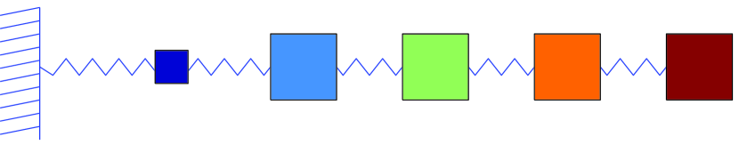
Fig. 4: A mechanical system consisting of $N=5$ masses attached with springs.

If we choose one of the masses to be much smaller than the others, $m_{1}=10^{-4}$ and $m_{2}=m_{3}=\cdots=m_{N}=1$, then we expect the dynamics of the system to be dominated by the smallest mass, in the sense that the resolution needed to compute the solution will be completely determined by the fast oscillations of the smallest mass.

To compare the multi-adaptive method with a standard method, we first compute with constant time-steps $k=k_{0}$ using the standard $\mathrm{cG}(1)$ method and measure the error, the cpu time needed to obtain the solution, the total number of steps, i.e., $M=\sum_{i=1}^{N}M_{i}$, and the number of local function evaluations. We then compute the solution with individual time-steps, using the $\mathrm{mcG}(1)$ method, choosing the time-steps $k_{i}=k_{0}$ for the position and velocity components of the smallest mass, and choosing $k_{i}=100k_{0}$ for the other components (knowing that the frequency of the oscillations scales like $1/\sqrt{m}$). For demonstration purposes, we thus choose the time-steps a priori to fit the dynamics of the system.

We repeat the experiment for increasing values of $N$ (see Figure 5) and find that the error is about the same and constant for both methods. As $N$ increases, the total number of time-steps, the number of local function evaluations (including also residual evaluations), and the cpu time increase linearly for the standard method, as we expect. For the multi-adaptive method, on the other hand, the total number of time-steps and local function evaluations remains practically constant as we increase $N$. The cpu time increases somewhat, since the increasing size of the time-slabs introduces some overhead, although not nearly as much as for the standard method. For this particular problem the gain of the multi-adaptive method is thus a factor $N$, where $N$ is the size of the system, so that by considering a large-enough system, the gain is arbitrarily large.

\psfrag{e}{$\|e(T)\|_{\infty}$}\psfrag{cpu time}{{cpu time / seconds}}\psfrag{function evaluations}{{function evaluations}}\psfrag{steps}{{steps}}\includegraphics[width=433.62pt,height=278.83708pt]{eps/multiadaptivity-20.eps}

\psfrag{e}{$\|e(T)\|_{\infty}$}\psfrag{cpu time}{{cpu time / seconds}}\psfrag{function evaluations}{{function evaluations}}\psfrag{steps}{{steps}}\includegraphics[width=433.62pt,height=278.83708pt]{eps/multiadaptivity-100-new.eps}

Fig. 5: Error, cpu time, total number of steps, and number of function evaluations as function of the number of masses for the multi-adaptive $\mathrm{cG}(1)$ method (dashed lines) and the standard $\mathrm{cG}(1)$ method (solid lines).

5.2 The Lorenz system

We consider now the famous Lorenz system,

(16) $$\left\{\begin{array}[]{rcl}\dot{x}&=&\sigma(y-x),\\ \dot{y}&=&rx-y-xz,\\ \dot{z}&=&xy-bz,\\ \end{array}\right.$$

with the usual data $(x(0),y(0),z(0))=(1,0,0)$, $\sigma=10$, $b=8/3$, and $r=28$; see [5]. The solution $u(t)=(x(t),y(t),z(t))$ is very sensitive to perturbations and is often described as “chaotic.” With our perspective this is reflected by stability factors with rapid growth in time.

The computational challenge is to solve the Lorenz system accurately on a time-interval $[0,T]$ with $T$ as large as possible. In Figure 6 is shown a computed solution which is accurate on the interval $[0,40]$. We investigate the computability of the Lorenz system by solving the dual problem and computing stability factors to find the maximum value of $T$. The focus in this section is not on multi-adaptivity—we will use the same time-steps for all components, and so $\mathrm{mcG}(q)$ becomes $\mathrm{cG}(q)$—but on higher-order methods and the precise information that can be obtained about the computability of a system from solving the dual problem and computing stability factors.

\psfrag{x}{$x$}\psfrag{z}{$z$}\psfrag{U}{$U$}\psfrag{t}{$t$}\includegraphics[width=433.62pt]{eps/lorenz-trajectory.eps}

Fig. 6: On the right is the trajectory of the Lorenz system for final time $T=40$, computed with the multi-adaptive $\mathrm{cG}(5)$ method. On the left is a plot of the time variation of the three components.

As an illustration, we present in Figure 7 solutions obtained with different methods and constant time-step $k=0.1$ for all components. For the lower-order methods, $\mathrm{cG}(5)$ to $\mathrm{cG}(11)$, it is clear that the error decreases as we increase the order. Starting with the $\mathrm{cG}(12)$ method, however, the error does not decrease as we increase the order. To explain this, we note that in every time-step a small round-off error of size $\sim 10^{-16}$ is introduced if the computation is carried out in double precision arithmetic. These errors accumulate at a rate determined by the growth of the stability factor for the computational error (see [10]). As we shall see below, this stability factor grows exponentially for the Lorenz system and reaches a value of $10^{16}$ at final time $T=50$, and so at this point the accumulation of round-off errors results in a large computational error.

\psfrag{cG(5)}{$\mathrm{cG}(5)$}\psfrag{cG(6)}{$\mathrm{cG}(6)$}\psfrag{cG(7)}{$\mathrm{cG}(7)$}\psfrag{cG(8)}{$\mathrm{cG}(8)$}\psfrag{cG(9)}{$\mathrm{cG}(9)$}\psfrag{cG(10)}{$\mathrm{cG}(10)$}\psfrag{cG(11)}{$\mathrm{cG}(11)$}\psfrag{cG(12)}{$\mathrm{cG}(12)$}\psfrag{cG(13)}{$\mathrm{cG}(13)$}\psfrag{cG(14)}{$\mathrm{cG}(14)$}\psfrag{cG(15)}{$\mathrm{cG}(15)$}\psfrag{t}{}\includegraphics[width=355.65944pt]{eps/lorenz-higher_order_1.eps}

\psfrag{cG(5)}{$\mathrm{cG}(5)$}\psfrag{cG(6)}{$\mathrm{cG}(6)$}\psfrag{cG(7)}{$\mathrm{cG}(7)$}\psfrag{cG(8)}{$\mathrm{cG}(8)$}\psfrag{cG(9)}{$\mathrm{cG}(9)$}\psfrag{cG(10)}{$\mathrm{cG}(10)$}\psfrag{cG(11)}{$\mathrm{cG}(11)$}\psfrag{cG(12)}{$\mathrm{cG}(12)$}\psfrag{cG(13)}{$\mathrm{cG}(13)$}\psfrag{cG(14)}{$\mathrm{cG}(14)$}\psfrag{cG(15)}{$\mathrm{cG}(15)$}\psfrag{t}{}\includegraphics[width=355.65944pt]{eps/lorenz-higher_order_2.eps}

Fig. 7: Solutions for the $x$-component of the Lorenz system with methods of different order, using a constant time-step $k=0.1$. Dotted lines indicate the point beyond which the solution is no longer accurate.

5.2.1 Stability factors

\psfrag{t}{$T$}\psfrag{S0}{$\bar{S}^{[0]}(T)$}\psfrag{25}{}\includegraphics[width=433.62pt]{eps/lorenz-stabilityfactor_0.eps}

Fig. 8: The stability factor for computational and quadrature errors, as function of time for the Lorenz system.

We now investigate the computation of stability factors for the Lorenz system. For simplicity we focus on global stability factors, such as

(17) $$S^{[q]}(T)=\max_{\|v\|=1}\int_{0}^{T}\|\varphi^{(q)}(t)\|\ dt,$$

where $\varphi(t)$ is the solution of the dual problem obtained with $\varphi(T)=v$ (and $g=0$). Letting $\Phi(t)$ be the fundamental solution of the dual problem, we have

(18) $$\ \ \,\qquad\max_{\|v\|=1}\int_{0}^{T}\|\Phi^{(q)}(t)v\|\ dt\leq\int_{0}^{T}\max_{\|v\|=1}\|\Phi^{(q)}(t)v\|\ dt=\int_{0}^{T}\|\Phi^{(q)}(t)\|\ dt\!=\!\bar{S}^{[q]}(T).$$

This gives a bound $\bar{S}^{[q]}(T)$ for $S^{[q]}(T)$, which for the Lorenz system turns out to be quite sharp and which is simpler to compute since we do not have to compute the maximum in (17).

In Figure 8 we plot the growth of the stability factor for $q=0$, corresponding to computational and quadrature errors as described in [10]. The stability factor grows exponentially with time, but not as fast as indicated by an a priori error estimate. An a priori error estimate indicates that the stability factors grow as

(19) $$S^{[q]}(T)\sim\mathcal{A}^{q}e^{\mathcal{A}T},$$

where $\mathcal{A}$ is a bound for the Jacobian of the right-hand side for the Lorenz system. A simple estimate is $\mathcal{A}=50$, which already at $T=1$ gives $S^{[0]}(T)\approx 10^{22}$. In view of this, we would not be able to compute even to $T=1$, and certainly not to $T=50$, where we have $S^{[0]}(T)\approx 10^{1000}$. The point is that although the stability factors grow very rapidly on some occasions, such as near the first flip at $T=18$, the growth is not monotonic. The stability factors thus effectively grow at a moderate exponential rate.

5.2.2 Conclusions

To predict the computability of the Lorenz system, we estimate the growth rate of the stability factors. A simple approximation of this growth rate, obtained from numerically computed solutions of the dual problem, is

(20) $$\bar{S}^{[q]}(T)\approx 4\cdot 10^{(q-3)+0.37T}$$

or just

(21) $$\bar{S}^{[q]}(T)\approx 10^{q+T/3}.$$

From the a posteriori error estimates presented in [10], we find that the computational error can be estimated as

(22) $$E_{C}\approx S^{[0]}(T)\max_{[0,T]}\|\mathcal{R}^{\mathcal{C}}\|,$$

where the computational residual $\mathcal{R}^{\mathcal{C}}$ is defined as

(23) $$\mathcal{R}^{\mathcal{C}}_{i}(t)=\frac{1}{k_{ij}}\left(U(t_{ij})-U(t_{i,j-1})-\int_{I_{ij}}f_{i}(U,\cdot)\ dt\right).$$

With 16 digits of precision a simple estimate for the computational residual is $\frac{1}{k_{ij}}\!10^{-16}$, which gives the approximation

(24) $$E_{C}\approx 10^{T/3}\frac{1}{\min k_{ij}}10^{-16}=10^{T/3-16}\frac{1}{\min k_{ij}}.$$

With time-steps $k_{ij}=0.1$ as above we then have

(25) $$E_{C}\approx 10^{T/3-15},$$

and so already at time $T=45$ we have $E_{C}\approx 1$ and the solution is no longer accurate. We thus conclude by examination of the stability factors that it is difficult to reach beyond time $T=50$ in double precision arithmetic. (With quadruple precision we would be able to reach time $T=100$.)

5.3 The solar system

We now consider the solar system, including the Sun, the Moon, and the nine planets, which is a particularly important $n$-body problem of the form

(26) $$m_{i}\ddot{x}_{i}=\sum_{j\neq i}\frac{Gm_{i}m_{j}}{|x_{j}-x_{i}|^{3}}(x_{j}-x_{i}),$$

where $x_{i}(t)=(x_{i}^{1}(t),x_{i}^{2}(t),x_{i}^{3}(t))$ denotes the position of body $i$ at time $t$, $m_{i}$ is the mass of body $i$, and $G$ is the gravitational constant.

As initial conditions we take the values at 00.00 Greenwich mean time on January 1, 2000, obtained from the United States Naval Observatory [2], with initial velocities obtained by fitting a high-degree polynomial to the values of December 1999. This initial data should be correct to five or more digits, which is similar to the available precision for the masses of the planets. We normalize length and time to have the space coordinates per astronomical unit, AU, which is (approximately) the mean distance between the Sun and Earth, the time coordinates per year, and the masses per solar mass. With this normalization, the gravitational constant is $4\pi^{2}$.

5.3.1 Predictability

Investigating the predictability of the solar system, the question is how far we can accurately compute the solution, given the precision in initial data. In order to predict the accumulation rate of errors, we solve the dual problem and compute stability factors. Assuming the initial data is correct to five or more digits, we find that the solar system is computable on the order of 500 years. Including also the Moon, we cannot compute more than a few years. The dual solution grows linearly backward in time (see Figure 9), and so errors in initial data grow linearly with time. This means that for every extra digit of increased precision, we can reach 10 times further.

\psfrag{v}{$\varphi$}\psfrag{t}{$t$}\includegraphics[width=433.62pt]{eps/earth-moon-dual.eps}

Fig. 9: Part of the dual of the solar system with data chosen for control of the error in the position of the moon at final time.

5.3.2 Computability

To touch briefly on the fundamental question of the computability of the solar system, concerning how far the system is computable with correct initial data and correct model, we compute the trajectories for Earth, the Moon, and the Sun over a period of $50$ years, comparing different methods. Since errors in initial data grow linearly, we expect numerical errors as well as stability factors to grow quadratically.

\psfrag{cG1}{$\mathrm{cG}(1)$}\psfrag{cG2}{$\mathrm{cG}(2)$}\psfrag{dG1}{$\mathrm{dG}(1)$}\psfrag{dG2}{$\mathrm{dG}(2)$}\psfrag{e}{$e$}\psfrag{t}{$t$}\includegraphics[width=433.62pt]{eps/earth-moon-computability.eps}

Fig. 10: The growth of the error over $50$ years for the Earth–Moon–Sun system as described in the text.

In Figure 10 we plot the errors for the $18$ components of the solution, computed for $k=0.001$ with $\mathrm{cG}(1)$, $\mathrm{cG}(2)$, $\mathrm{dG}(1)$, and $\mathrm{dG}(2)$. This figure contains much information. To begin with, we see that the error seems to grow linearly for the $\mathrm{cG}$ methods. This is in accordance with earlier observations [4, 7] for periodic Hamiltonian systems, recalling that the $\mathrm{(m)cG}(q)$ methods conserve energy [10]. The stability factors, however, grow quadratically and thus overestimate the error growth for this particular problem. In an attempt to give an intuitive explanation of the linear growth, we may think of the error introduced at every time-step by an energy-conserving method as a pure phase error, and so at every time-step the Moon is pushed slightly forward along its trajectory (with the velocity adjusted accordingly). Since a pure phase error does not accumulate but stays constant (for a circular orbit), the many small phase errors give a total error that grows linearly with time.

Examining the solutions obtained with the $\mathrm{dG}(1)$ and $\mathrm{dG}(2)$ methods, we see that the error grows quadratically, as we expect. For the $\mathrm{dG}(1)$ solution, the error reaches a maximum level of $\sim 0.5$ for the velocity components of the Moon. The error in position for the Moon is much smaller. This means that the Moon is still in orbit around Earth, the position of which is still very accurate, but the position relative to Earth, and thus also the velocity, is incorrect. The error thus grows quadratically until it reaches a limit. This effect is also visible for the error of the $\mathrm{cG}(1)$ solution; the linear growth flattens out as the error reaches the limit. Notice also that even if the higher-order $\mathrm{dG}(2)$ method performs better than the $\mathrm{cG}(1)$ method on a short time-interval, it will be outrun on a long enough interval by the $\mathrm{cG}(1)$ method, which has linear accumulation of errors (for this particular problem).

\psfrag{e}{$e$}\psfrag{k}{$k$}\psfrag{t}{$t$}\psfrag{t1}{\footnotesize All components}\psfrag{t2}{\footnotesize Position of the Moon}\includegraphics[width=433.62pt]{eps/earth-moon-computability-multiadaptive.eps}

Fig. 11: The growth of the error over $5$ years for the Earth–Moon–Sun system computed with the $\mathrm{mcG}(2)$ method, together with the multi-adaptive time-steps.

5.3.3 Multi-adaptive time-steps

Solving with the multi-adaptive method $\mathrm{mcG}(2)$ (see Figure 11), the error grows quadratically. We saw in [10] that in order for the $\mathrm{mcG}(q)$ method to conserve energy, we require that corresponding position and velocity components use the same time-steps. Computing with different time-steps for all components, as here, we thus cannot expect to have linear error growth. Keeping $k_{i}^{2}r_{i}\leq\mathrm{tol}$ with $\mathrm{tol}=10^{-10}$ as here, the error grows as $10^{-4}T^{2}$ and we are able to reach $T\sim 100$. Decreasing $\mathrm{tol}$ to, say, $10^{-18}$, we could instead reach $T\sim 10^{6}$.

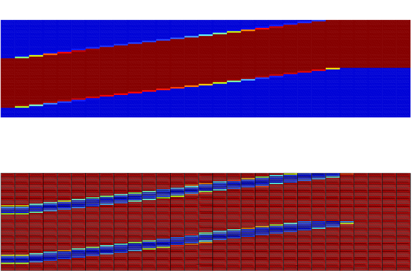
Fig. 12: A space-time plot of the solution (above) and time-steps (below) for the propagating front problem, with time going to the right. The two parts of the plots represent the components for the two species $A_{1}$ (lower parts) and $A_{2}$ (upper parts).

We investigated the passing of a large comet close to Earth and the Moon and found that the stability factors increase dramatically at the time $t^{\prime}$ when the comet comes very close to the Moon. The conclusion is that if we want to compute accurately to a point beyond $t^{\prime}$, we have to be much more careful than if we want to compute to a point just before $t^{\prime}$. This is not evident from the size of residuals or local errors. This is an example of a Hamiltonian system for which the error growth is neither linear nor quadratic.

5.4 A propagating front problem

The system of PDEs

(27) $$\left\{\begin{array}[]{rcl}\dot{u}_{1}-\epsilon u_{1}^{\prime\prime}&=&-u_{1}u_{2}^{2},\\ \dot{u}_{2}-\epsilon u_{2}^{\prime\prime}&=&u_{1}u_{2}^{2}\end{array}\right.$$

on $(0,1)\times(0,T]$ with $\epsilon=0.00001$, $T=100$, and homogeneous Neumann boundary conditions at $x=0$ and $x=1$ models isothermal autocatalytic reactions (see [14]) $A_{1}+2A_{2}\rightarrow A_{2}+2A_{2}$. We choose the initial conditions as

$$u_{1}(x,0)=\left\{\begin{array}[]{ll}0,&x<x_{0},\\ 1,&x\geq x_{0},\end{array}\right.$$

with $x_{0}=0.2$ and $u_{2}(x,0)=1-u_{1}(x,0)$. An initial reaction where substance $A_{1}$ is consumed and substance $A_{2}$ is formed will then occur at $x=x_{0}$, resulting in a decrease in the concentration $u_{1}$ and an increase in the concentration $u_{2}$. The reaction then propagates to the right until all of substance $A_{1}$ is consumed and we have $u_{1}=0$ and $u_{2}=1$ in the entire domain.

Solving with the $\mathrm{mcG}(2)$ method, we find that the time-steps are small only close to the reaction front; see Figures 12 and 13. The reaction front propagates to the right as does the domain of small time-steps.

It is clear that if the reaction front is localized in space and the domain is large, there is a lot to gain by using small time-steps only in this area. To verify this, we compute the solution to within an accuracy of $10^{-7}$ for the final time error with constant time-steps $k_{i}(t)=k_{0}$ for all components and compare with the multi-adaptive solution. Computing on a space grid consisting of $16$ nodes on $[0,1]$ (resulting in a system of ODEs with $32$ components), the solution is computed in $2.1$ seconds on a regular workstation. Computing on the same grid with the multi-adaptive method (to within the same accuracy), we find that the solution is computed in $3.0$ seconds. More work is thus required to compute the multi-adaptive solution, and the reason is the overhead resulting from additional bookkeeping and interpolation in the multi-adaptive computation. However, increasing the size of the domain to $32$ nodes on $[0,2]$ and keeping the same parameters otherwise, we find the solution is now more localized in the domain and we expect the multi-adaptive method to perform better compared to a standard method. Indeed, the computation using equal time-steps now takes $5.7$ seconds, whereas the multi-adaptive solution is computed in $3.4$ seconds. In the same way as previously shown in section 5.1, adding extra degrees of freedom does not substantially increase the cost of solving the problem, since the main work is done time-stepping the components, which use small time-steps.

\psfrag{x}{$x$}\psfrag{U1}{$U_{1}$}\psfrag{U2}{$U_{2}$}\psfrag{k1}{$k_{1}$}\psfrag{k2}{$k_{2}$}\includegraphics[width=433.62pt]{eps/front_solution_50.eps}

Fig. 13: The concentrations of the two species $U_{1}$ and $U_{2}$ at time $t=50$ as function of space (above) and the corresponding time-steps (below).

5.5 Burger’s equation with moving nodes

As a final example, we present a computation in which we combine multi-adaptivity with the possibility of moving the nodes in a space discretization of a time-dependent PDE. Solving Burger’s equation,

(28) $$\dot{u}+\mu uu^{\prime}-\epsilon u^{\prime\prime}=0,$$

on $(0,1)\times(0,T]$ with initial condition

(29) $$u_{0}(x)=\left\{\begin{array}[]{ll}\sin(\pi x/x_{0}),&0\leq x\leq x_{0},\\ 0&\mbox{elsewhere},\end{array}\right.$$

and with $\mu=0.1$, $\epsilon=0.001$, and $x_{0}=0.3$, we find the solution is a shock forming near $x=x_{0}$. Allowing individual time-steps within the domain, and moving the nodes of the space discretization in the direction of the convection, $(1,\mu u)$, we make the ansatz

(30) $$U(x,t)=\sum_{i=1}^{N}\xi_{i}(t)\varphi_{i}(x,t),$$

where the $\{\xi_{i}\}_{i=1}^{N}$ are the individual components computed with the multi-adaptive method, and the $\{\varphi_{i}(\cdot,t)\}_{i=1}^{N}$ are piecewise linear basis functions in space for any fixed $t$.

Solving with the $\mathrm{mdG}(0)$ method, the nodes move into the shock, in the direction of the convection, so what we are really solving is a heat equation with multi-adaptive time-steps along the streamlines; see Figures 14 and 15.

\psfrag{x}{$x$}\psfrag{U(x)}{$U(x)$}\includegraphics[width=433.62pt]{eps/burger-solutions.eps}

Fig. 14: The solution to Burger’s equation as function of space at $t=0$, $t=T/2$, and $t=T$.

\psfrag{x}{$x$}\psfrag{t}{$t$}\includegraphics[width=433.62pt]{eps/burger-paths_2.eps}

Fig. 15: Node paths for the multi-adaptive moving-nodes solution of Burger’s equation.

6 Future work

Together with the companion paper [10] (see also [9, 8]), this paper serves as a starting point for further investigation of the multi-adaptive Galerkin methods and their properties.

Future work will include a more thorough investigation of the application of the multi-adaptive methods to stiff ODEs, as well as the construction of efficient multi-adaptive solvers for time-dependent PDEs, for which memory usage becomes animportant issue.

References

- [1] GNU Project Web Server, http://www.gnu.org/.
- [2] USNO Astronomical Applications Department, http://aa.usno.navy.mil/.
- [3] K. Eriksson, C. Johnson, and A. Logg, Explicit time-stepping for stiff ODEs, SIAM J. Sci. Comput., 25 (2003), pp. 1142–1157.
- [4] D. Estep, The rate of error growth in Hamiltonian-conserving integrators, Z. Angew. Math. Phys., 46 (1995), pp. 407–418.
- [5] D. Estep and C. Johnson, The computability of the Lorenz system, Math. Models Methods Appl. Sci., 8 (1998), pp. 1277–1305.
- [6] K. Gustafsson, M. Lundh, and G. Söderlind, A pi stepsize control for the numerical solution of ordinary differential equations, BIT, 28 (1988), pp. 270–287.
- [7] M. G. Larson, Error growth and a posteriori error estimates for conservative Galerkin approximations of periodic orbits in Hamiltonian systems, Math. Models Methods Appl. Sci., 10 (2000), pp. 31–46.
- [8] A. Logg, Multi-Adaptive Error Control for ODEs, Preprint 2000-03, Chalmers Finite Element Center, Chalmers University of Technology, Göteborg, Sweden, 2000. Also available online from http://www.phi.chalmers.se/preprints/.
- [9] A. Logg, A Multi-Adaptive ODE-Solver, Preprint 2000-02, Chalmers Finite Element Center, Chalmers University of Technology, Göteborg, Sweden, 2000. Also available online from http://www.phi.chalmers.se/preprints/.
- [10] A. Logg, Multi-adaptive Galerkin methods for ODEs I, SIAM J. Sci. Comput., 24 (2003), pp. 1879–1902.
- [11] A. Logg, Multi-Adaptive Galerkin Methods for ODEs II: Applications, Preprint 2001-10, Chalmers Finite Element Center, Chalmers University of Technology, Göteborg, Sweden, 2001. Also available online from http://www.phi.chalmers.se/preprints/.
- [12] A. Logg, Tanganyika, Version 1.2, 2001. http://www.phi.chalmers.se/tanganyika/.
- [13] W. Press, S. Teukolsky, W. Vetterling, and B. Flannery, Numerical Recipes in C. The Art of Scientific Computing, 2nd ed., Cambridge University Press, Cambridge, UK, 1992. Also available online from http://www.nr.com.
- [14] R. Sandboge, Adaptive Finite Element Methods for Reactive Flow Problems, Ph.D. thesis, Department of Mathematics, Chalmers University of Technology, Göteborg, Sweden, 1996.
- [15] G. Söderlind, The automatic control of numerical integration. Solving differential equations on parallel computers, CWI Quarterly, 11 (1998), pp. 55–74.