Solution of 2D Boussinesq systems with FreeFem++: the flat bottom case

Abstract - We consider here different family of Boussinesq systems in two space dimensions. These systems approximate the three-dimensional Euler equations and consist of three coupled nonlinear dispersive wave equations that describe propagation of long surface waves of small amplitude in ideal fluids over a horizontal bottom and which was studied in [7, 9, 10]. We present here a # FreeFem ++ code aimed at solving numerically these systems where a discretization using $\mathbb{P}_{1}$ finite element for these systems was taken in space and a second order Runge-Kutta scheme in time. We give the detail of our code where we use a mesh adaptation technique. An optimization of the used algorithm is done and a comparison of the solution for different Boussinesq family is done too. The results we obtained agree with those of the literature.

Keywords: Boussinesq systems, KdV-KdV, BBM-BBM, Bona-Smith, adaptmesh, finite element method, FreeFem++.

1 Introduction

It has often been observed that variations of the bottom could influence the damping of the waves including extreme ones as Tsunamis: the coral reef or the underwater forests in the first shoreline, mangroves; these underwater reefs are also used to prevent corrosion effects of coastal (see P. Azerad et al. [1] and [2]). In these cases, the underwater relief damped the wave energy, in contrast, in other situations we seek to harness this energy: some companies even offer projects underwater reefs for erectile produce energy from waves (see http://www.aquamarinepower.com/).

In a continuum approximation, waves on the surface of an ideal fluid under the force of gravity are governed by the Euler equations. These are expected to provide a good model of irrotational waves on the surface of water, say, in situations where dissipative and surface tension effects may be safely ignored, see [16].

In this paper, the attention is given to a multi-dimensional Boussinesq systems which describes approximately the propagation of small amplitude and long wave-length surface waves in a three-dimensional wave tank filled with an irrotational, incompressible and inviscid liquid under the influence of gravity, moving and/or variable bottom and surface pressure. The full Boussinesq systems in 2D has been derived in [18].

Chen, Goubet, Dougalis, Mitsotakis and Saut have considered 2D models of Boussinesq systems with flat bottom [7, 9] then with variable bottom [6, 12, 17], on the other hand Dutykh, Katsaounis and Mitsotakis have developed a code in finite volumes for the Boussinesq systems with variable bottom in 1D ([13]) and Mitsotakis et al. in Galerkin finite elements (using B-splines [9]).

In order to solve numerically the Boussinesq system, we will use # FreeFem ++ which is an open source platform to solve partial differential equations numerically, based on finite element methods. The # FreeFem ++ platform has been developed to facilitate teaching and basic research through prototyping. For the moment this platform is restricted to the numerical simulations of problems which admit a variational formulation.

Thus, we develop a # FreeFem ++ code for the simulation of Boussinesq equations with flat bottom, we first check that the simulations provided by our numerical code are consistent with the results of the recent literature, including the work of Dougalis, Mitsotakis et Saut [9, 10, 11]. This establishes the adequacy of the chosen finite element discretization.

The article is organized as follows: first we discretize the problem in space by using finite element method and in time by using an explicit second order Runge-Kutta scheme, then we develop all the steps of the # FreeFem ++ code to solve the problem by using the technique of mesh adaptation and at the end we present some numerical results where an optimization of the used algorithm is done and a comparison of the solution for different Boussinesq family is done too.

2 The Problem

2.1 Problem settings

The 2D Boussineq system describe the surface wave propagation of small amplitude and large wave length. When considering an incompressible fluid flows in $\Omega\subset\mathbb{R}^{2}$, they are expressed as (see [16]):

$$\begin{array}[]{rcl}\eta_{t}+\nabla\cdot\textbf{V}+\nabla\cdot(\eta\textbf{V})+a\Delta\nabla\cdot\textbf{V}-b\Delta\eta_{t}&=&0;\\ \\ \textbf{V}_{t}+\nabla\eta+\frac{1}{2}\nabla|\textbf{V}|^{2}+c\Delta\nabla\eta-d\Delta\textbf{V}_{t}&=&0,\end{array}$$ (2.1)

The variables in (2.1) are non-dimensional and unscaled: $\textbf{X}=(x,y)\in\Omega$ and $t>0$ are proportional to position along the channel and time, respectively, $\eta=\eta(\textbf{X},t)$ is proportional to the deviation of the free surface from its rest position, $\textbf{V}=\textbf{V}(\textbf{X},t)=\left(\begin{array}[]{c}u(\textbf{X},t)\\ v(\textbf{X},t)\end{array}\right)=(u,v)^{T}=(u;v)$ is proportional to the horizontal velocity of the fluid at some height, $\nabla\textbf{*}=\left(\begin{array}[]{c}\partial_{x}\textbf{*}\\ \partial_{y}\textbf{*}\end{array}\right)$ is the gradient, $\nabla\cdot\left(\begin{array}[]{c}\star\\ \textbf{*}\end{array}\right)=\partial_{x}\star+\partial_{y}\textbf{*}$ is the divergence and $\Delta\textbf{*}=\partial_{xx}\textbf{*}+\partial_{yy}\textbf{*}$ is the laplacian. The coefficients $a,b,c$ and $d$ are given by the following formulas:

$$a=\frac{1}{2}\left(\vartheta^{2}-\frac{1}{3}\right)\nu,b=\frac{1}{2}\left(\vartheta^{2}-\frac{1}{3}\right)(1-\nu),c=\frac{1}{2}\left(1-\vartheta^{2}\right)\mu,d=\frac{1}{2}\left(1-\vartheta^{2}\right)(1-\mu)$$ (2.2)

where $\nu,\mu$ are real constants and $0\leqslant\vartheta\leqslant 1$.
We note that the dispersive constants $a,b,c$ and $d$ satisfy the physical constraints (see [3] for detail):

$$a+b+c+d=\frac{1}{3}\mbox{ and }c+d\geqslant 0$$ (2.3)

We now list some of the different family of Boussinesq systems 2D in Table 1 of the form (2.1):

System	$\vartheta^{2}$	$\nu$	$\mu$	References
BBM-BBM	$2/3$	$0$	$0$	[6, 7, 9, 10, 11].
Bona-Smith	$2/3\leqslant\vartheta^{2}\leqslant 1$	$0$	$\displaystyle\frac{4-6\vartheta^{2}}{3(1-\vartheta^{2})}$	[7, 9, 10, 11].
“ General ” Boussinesq	$0\leqslant\vartheta^{2}\leqslant 1$	any	any	[7, 9, 11].
KdV-KdV	$2/3$	$1$	$1$	[14]

Table 1: Examples of Boussinesq systems in 2D.

In [9], V. Dougalis, D. Mitsotakis and J-C. Saut have studied the Well-Posedness of the Boussinesq systems (2.1) (where $b\neq 0$ and $d\neq 0$) and have shown that this system is at least nonlinearly well-posed locally; and in the case of KdV-KdV system (where $b=d=0,a=c=1/6$), F. Linares, D. Pilod and J-C. Saut proved recently in [14] the Well-Posedness of this system.

Following [19], we can write (2.1) as:

$$\begin{array}[]{rcl}\Upsilon-\Delta\textbf{V}&=&0;\\ \\ \eta_{t}+\nabla\cdot\textbf{V}+\nabla\cdot(\eta\textbf{V})+a\nabla\cdot\Upsilon-b\Delta\eta_{t}&=&0;\\ \\ \Theta-\Delta\eta&=&0;\\ \\ \textbf{V}_{t}+\nabla\eta+\frac{1}{2}\nabla|\textbf{V}|^{2}+c\nabla\Theta-d\Delta\textbf{V}_{t}&=&0,\end{array}$$ (2.4)

where $\Upsilon=\left(\Upsilon^{1},\Upsilon^{2}\right)^{T}=\left(\Upsilon^{1};\Upsilon^{2}\right)$.

3 Numerical Scheme

In this section, we present the spatial discretization using finite element method with $\mathbb{P}_{1}$ continuous piecewise linear functions as shown in [19] and for the time marching scheme an explicit second order Runge-Kutta [8] scheme as used in [9].
We will use in our code a mesh adaptation technic that we can use solving the problem by using the method based on the declaration of the problem obtained by the weak formulation of the system (2.4); or by using the second method that consist to build matrices and vectors to solve the direct system $\mathbf{A}\mathbf{X}=\mathbf{B}$, where the matrix $\mathbf{A}$ and the vectors $\mathbf{X},\mathbf{B}$ will be defined in the sequel.

3.1 Spatial discretization

We let $\Omega$ be a convex, plane domain, let $\mathbf{T}_{h}$ denote a regular, quasi uniform triangulation of $\Omega$ with triangles of maximum size $h<1$ [5], let $V_{h}=\{v_{h}\in C^{0}(\bar{\Omega});v_{h}|_{T}\in\mathbb{P}_{1}(T),\forall T\in\mathbf{T}_{h}\}$ denote a finite-dimensional subspace of $H^{1}(\Omega)=\{u\in L^{2}(\Omega)\mbox{ s.t. }\frac{\partial u}{\partial x},\frac{\partial u}{\partial y}\in L^{2}(\Omega)\}$ where $\mathbb{P}_{1}$ is the set of polynomials of $\mathbb{R}$ of degrees $\leqslant 1$ and let $\left\langle\cdot;\cdot\right\rangle$ denote the $L^{2}$ inner product on $\Omega$.
Consider the weak formulation of the system (2.4), find $\eta_{h},u_{h},v_{h}\in V_{h}$ such that $\forall\varphi_{h}\in V_{h}$ we have:

$$\begin{array}[]{rcl}\left\langle\Upsilon^{1}_{h};\varphi_{h}\right\rangle-\left\langle\Delta u_{h};\varphi_{h}\right\rangle=0;\quad\left\langle\Upsilon^{2}_{h};\varphi_{h}\right\rangle-\left\langle\Delta v_{h};\varphi_{h}\right\rangle=0;\quad\left\langle\Theta_{h};\varphi_{h}\right\rangle-\left\langle\Delta\eta_{h};\varphi_{h}\right\rangle&=&0;\\ \Big{\langle}(Id-b\Delta)\eta_{ht}+\nabla\cdot\left(u_{h};v_{h}\right)+\eta_{hx}u_{h}+\eta_{h}u_{hx}+\eta_{hy}u_{h}+\eta_{h}u_{hy}+a\nabla\cdot\left(\Upsilon^{1}_{h};\Upsilon^{2}_{h}\right);\varphi_{h}\Big{\rangle}&=&0;\\ \Big{\langle}(Id-d\Delta)u_{ht}+\eta_{hx}+u_{h}u_{hx}+v_{h}v_{hx}+c\Theta_{hx};\varphi_{h}\Big{\rangle}&=&0;\\ \Big{\langle}(Id-d\Delta)v_{ht}+\eta_{hy}+u_{h}u_{hy}+v_{h}v_{hy}+c\Theta_{hy};\varphi_{h}\Big{\rangle}&=&0.\end{array}$$ (3.5)

To simplify, we denote $\Phi=\varphi_{h},\mathbf{E}=\eta_{h},\mathbf{U}=u_{h},\mathbf{V}=v_{h},\mathbf{T}=\Theta_{h},\mathbf{P}=\Upsilon_{h}^{1}$ and $\mathbf{Q}=\Upsilon_{h}^{2}$, so the system (3.5) is equivalent to the following system:

$$\begin{array}[]{rcl}\lx@intercol\hfil\left\langle\mathbf{P};\Phi\right\rangle\quad=\quad\left\langle\Delta\mathbf{U};\Phi\right\rangle;\quad\left\langle\mathbf{Q};\Phi\right\rangle\quad=\quad\left\langle\Delta\mathbf{V};\Phi\right\rangle;\quad\left\langle\mathbf{T};\Phi\right\rangle\quad=\quad\left\langle\Delta\mathbf{E};\Phi\right\rangle;\hfil\lx@intercol\\ \Big{\langle}(Id-b\Delta)\partial_{t}\mathbf{E};\Phi\Big{\rangle}&=&-\left\langle\nabla\cdot(\mathbf{U};\mathbf{V})+\mathbf{E}_{x}\mathbf{U}+\mathbf{E}\mathbf{U}_{x}+\mathbf{E}_{y}\mathbf{V}+\mathbf{E}\mathbf{V}_{y}+a\nabla\cdot\left(\mathbf{P};\mathbf{Q}\right);\Phi\right\rangle\\ &=&-\mathbf{F}\left(\mathbf{E},\mathbf{U},\mathbf{V},\mathbf{P},\mathbf{Q}\right);\\ \Big{\langle}(Id-d\Delta)\partial_{t}\mathbf{U};\Phi\Big{\rangle}&=&-\left\langle\mathbf{E}_{x}+\mathbf{U}\mathbf{U}_{x}+\mathbf{V}\mathbf{V}_{x}+c\mathbf{T}_{x};\Phi\right\rangle=-\mathbf{G}\left(\mathbf{E},\mathbf{U},\mathbf{V},\mathbf{T}\right);\\ \Big{\langle}(Id-d\Delta)\partial_{t}\mathbf{V};\Phi\Big{\rangle}&=&-\left\langle\mathbf{E}_{y}+\mathbf{U}\mathbf{U}_{y}+\mathbf{V}\mathbf{V}_{y}+c\mathbf{T}_{y};\Phi\right\rangle=-\mathbf{H}\left(\mathbf{E},\mathbf{U},\mathbf{V},\mathbf{T}\right).\end{array}$$ (3.6)

3.2 Time marching scheme

Our method is based on an explicit second order Runge-Kutta scheme. To this end, let us denote by $(\mathbf{E}^{n+1},\mathbf{U}^{n+1},\mathbf{V}^{n+1})$ and $(\mathbf{E}^{n},\mathbf{U}^{n},\mathbf{V}^{n},\mathbf{P}^{n},\mathbf{Q}^{n},\mathbf{T}^{n})$ the approximate value at time $t=t^{n+1}$ and $t=t^{n}$, respectively and by $\delta t$ the time step size. Then, by using (3.6), the unknown fields at time $t=t^{n+1}$ are defined as the solution of the system

$$\left\{\begin{array}[]{l}\left\langle\mathbf{P}^{n};\Phi\right\rangle=\left\langle\Delta\mathbf{U}^{n};\Phi\right\rangle;\qquad\left\langle\mathbf{Q}^{n};\Phi\right\rangle=\left\langle\Delta\mathbf{V}^{n};\Phi\right\rangle;\qquad\left\langle\mathbf{T}^{n};\Phi\right\rangle=\left\langle\Delta\mathbf{E}^{n};\Phi\right\rangle;\\ \langle\mathbf{E}^{n+1};\Phi\rangle=\langle\mathbf{E}^{n}+\displaystyle\frac{\mathbf{E}^{k1}+\mathbf{E}^{k2}}{2};\Phi\rangle;\langle\mathbf{U}^{n+1};\Phi\rangle=\langle\mathbf{U}^{n}+\displaystyle\frac{\mathbf{U}^{k1}+\mathbf{U}^{k2}}{2};\Phi\rangle;\\ \langle\mathbf{V}^{n+1};\Phi\rangle=\langle\mathbf{V}^{n}+\displaystyle\frac{\mathbf{V}^{k1}+\mathbf{V}^{k2}}{2};\Phi\rangle.\end{array}\right.$$ (3.7)

where:

$$\left\{\begin{array}[]{l}\left\langle(Id-b\Delta)\mathbf{E}^{k1};\Phi\right\rangle=-\delta t\cdot\mathbf{F}\left(\mathbf{E}^{n},\mathbf{U}^{n},\mathbf{V}^{n},\mathbf{P}^{n},\mathbf{Q}^{n}\right);\\ \left\langle(Id-d\Delta)\mathbf{U}^{k1};\Phi\right\rangle=-\delta t\cdot\mathbf{G}\left(\mathbf{E}^{n},\mathbf{U}^{n},\mathbf{V}^{n},\mathbf{T}^{n}\right);\\ \left\langle(Id-d\Delta)\mathbf{V}^{k1};\Phi\right\rangle=-\delta t\cdot\mathbf{H}\left(\mathbf{E}^{n},\mathbf{U}^{n},\mathbf{V}^{n},\mathbf{T}^{n}\right);\\ \left\langle\mathbf{P}^{k1};\Phi\right\rangle=\left\langle\mathbf{U}^{k1}_{xx}+\mathbf{U}^{k1}_{yy};\Phi\right\rangle;\left\langle\mathbf{Q}^{k1};\Phi\right\rangle=\left\langle\mathbf{V}^{k1}_{xx}+\mathbf{V}^{k1}_{yy};\Phi\right\rangle;\left\langle\mathbf{T}^{k1};\Phi\right\rangle=\left\langle\mathbf{E}_{xx}^{k1}+\mathbf{E}_{yy}^{k1};\Phi\right\rangle.\end{array}\right.$$ (3.8)

and

$$\left\{\begin{array}[]{rcl}\left\langle(Id-b\Delta)\mathbf{E}^{k2};\Phi\right\rangle&=&-\delta t\cdot\mathbf{F}\left(\mathbf{E}^{n}+\mathbf{E}^{k1},\mathbf{U}^{n}+\mathbf{U}^{k1},\mathbf{V}^{n}+\mathbf{V}^{k1},\mathbf{P}^{n}+\mathbf{P}^{k1},\mathbf{Q}^{n}+\mathbf{Q}^{k1}\right);\\ \left\langle(Id-d\Delta)\mathbf{U}^{k2};\Phi\right\rangle&=&-\delta t\cdot\mathbf{G}\left(\mathbf{E}^{n}+\mathbf{E}^{k1},\mathbf{U}^{n}+\mathbf{U}^{k1},\mathbf{V}^{n}+\mathbf{V}^{k1},\mathbf{T}^{n}+\mathbf{T}^{k1}\right);\\ \left\langle(Id-d\Delta)\mathbf{V}^{k2};\Phi\right\rangle&=&-\delta t\cdot\mathbf{H}\left(\mathbf{E}^{n}+\mathbf{E}^{k1},\mathbf{U}^{n}+\mathbf{U}^{k1},\mathbf{V}^{n}+\mathbf{V}^{k1},\mathbf{T}^{n}+\mathbf{T}^{k1}\right).\end{array}\right.$$ (3.9)

By integrating by parts where we have second order derivative and by developing all the terms of the first order derivative in (3.7), (3.8) and (3.9), we deduce:

$$\begin{array}[]{c}\left\langle\mathbf{P}^{n};\Phi\right\rangle=-\left\langle\nabla\mathbf{U}^{n};\nabla\Phi\right\rangle+\left\langle\displaystyle\frac{\partial\mathbf{U}^{n}}{\partial n};\Phi\right\rangle_{\partial\Omega};\left\langle\mathbf{Q}^{n};\Phi\right\rangle=-\left\langle\nabla\mathbf{V}^{n};\nabla\Phi\right\rangle+\left\langle\displaystyle\frac{\partial\mathbf{V}^{n}}{\partial n};\Phi\right\rangle_{\partial\Omega};\\ \\ \left\langle\mathbf{T}^{n};\Phi\right\rangle=-\left\langle\nabla\mathbf{E}^{n};\nabla\Phi\right\rangle+\left\langle\displaystyle\frac{\partial\mathbf{E}^{n}}{\partial n};\Phi\right\rangle_{\partial\Omega};\end{array}$$ (3.10)

$$\left\{\begin{array}[]{rcl}\left\langle\mathbf{E}^{k1};\Phi\right\rangle+b\left\langle\nabla\mathbf{E}^{k1};\nabla\Phi\right\rangle-b\left\langle\displaystyle\frac{\partial\mathbf{E}^{k1}}{\partial n};\Phi\right\rangle_{\partial\Omega}&=&-\delta t\cdot\mathbf{F}\left(\mathbf{E}^{n},\mathbf{U}^{n},\mathbf{V}^{n},\mathbf{P}^{n},\mathbf{Q}^{n}\right);\\ \left\langle\mathbf{U}^{k1};\Phi\right\rangle+d\left\langle\nabla\mathbf{U}^{k1};\nabla\Phi\right\rangle-d\left\langle\displaystyle\frac{\partial\mathbf{U}^{k1}}{\partial n};\Phi\right\rangle_{\partial\Omega}&=&-\delta t\cdot\mathbf{G}\left(\mathbf{E}^{n},\mathbf{U}^{n},\mathbf{V}^{n},\mathbf{T}^{n}\right);\\ \left\langle\mathbf{V}^{k1};\Phi\right\rangle+d\left\langle\nabla\mathbf{V}^{k1};\nabla\Phi\right\rangle-d\left\langle\displaystyle\frac{\partial\mathbf{V}^{k1}}{\partial n};\Phi\right\rangle_{\partial\Omega}&=&-\delta t\cdot\mathbf{H}\left(\mathbf{E}^{n},\mathbf{U}^{n},\mathbf{V}^{n},\mathbf{T}^{n}\right);\\ \left\langle\mathbf{P}^{k1};\Phi\right\rangle=-\left\langle\nabla\mathbf{U}^{k1};\nabla\Phi\right\rangle+\left\langle\displaystyle\frac{\partial\mathbf{U}^{k1}}{\partial n};\Phi\right\rangle_{\partial\Omega};&&\\ \left\langle\mathbf{Q}^{k1};\Phi\right\rangle=-\left\langle\nabla\mathbf{V}^{k1};\nabla\Phi\right\rangle+\left\langle\displaystyle\frac{\partial\mathbf{V}^{k1}}{\partial n};\Phi\right\rangle_{\partial\Omega};&&\\ \left\langle\mathbf{T}^{k1};\Phi\right\rangle=-\left\langle\nabla\mathbf{E}^{k1};\nabla\Phi\right\rangle+\left\langle\displaystyle\frac{\partial\mathbf{E}^{k1}}{\partial n};\Phi\right\rangle_{\partial\Omega};&&\end{array}\right.$$ (3.11)

and

$$\left\{\begin{array}[]{l}\left\langle\mathbf{E}^{k2};\Phi\right\rangle+b\left\langle\nabla\mathbf{E}^{k2};\nabla\Phi\right\rangle-b\left\langle\displaystyle\frac{\partial\mathbf{E}^{k2}}{\partial n};\Phi\right\rangle_{\partial\Omega}=\\ \qquad\qquad\qquad-\delta t\cdot\mathbf{F}\left(\mathbf{E}^{n}+\mathbf{E}^{k1},\mathbf{U}^{n}+\mathbf{U}^{k1},\mathbf{V}^{n}+\mathbf{V}^{k1},\mathbf{P}^{n}+\mathbf{P}^{k1},\mathbf{Q}^{n}+\mathbf{Q}^{k1}\right);\\ \left\langle\mathbf{U}^{k2};\Phi\right\rangle+d\left\langle\nabla\mathbf{U}^{k2};\nabla\Phi\right\rangle-d\left\langle\displaystyle\frac{\partial\mathbf{U}^{k2}}{\partial n};\Phi\right\rangle_{\partial\Omega}=\\ \qquad\qquad\qquad-\delta t\cdot\mathbf{G}\left(\mathbf{E}^{n}+\mathbf{E}^{k1},\mathbf{U}^{n}+\mathbf{U}^{k1},\mathbf{V}^{n}+\mathbf{V}^{k1},\mathbf{T}^{n}+\mathbf{T}^{k1}\right);\\ \left\langle\mathbf{V}^{k2};\Phi\right\rangle+d\left\langle\nabla\mathbf{V}^{k2};\nabla\Phi\right\rangle-d\left\langle\displaystyle\frac{\partial\mathbf{V}^{k2}}{\partial n};\Phi\right\rangle_{\partial\Omega}=\\ \qquad\qquad\qquad-\delta t\cdot\mathbf{H}\left(\mathbf{E}^{n}+\mathbf{E}^{k1},\mathbf{U}^{n}+\mathbf{U}^{k1},\mathbf{V}^{n}+\mathbf{V}^{k1},\mathbf{T}^{n}+\mathbf{T}^{k1}\right).\end{array}\right.$$ (3.12)

Remark: It’s easy with # FreeFem ++ to define boundary condition, in fact if we have the Dirichlet Boundary Conditions on a border $\Gamma_{1}\subset\mathbb{R}$ like $\mathbf{U}|_{\Gamma_{1}}=f$, then it is defined as on(gamma1,u=f), where u is the unknown function in the problem. We note that the Neumann Boundary Conditions on $\Gamma_{2}\subset\mathbb{R}$, like $\displaystyle\frac{\partial\mathbf{U}}{\partial n}|_{\Gamma_{2}}=g$, appear in the Weak formulation of the problem after integrating by parts for example in the system (3.10) we have $\left\langle\displaystyle\frac{\partial\mathbf{U}}{\partial n};\Phi\right\rangle_{\Gamma_{2}}=\left\langle g;\Phi\right\rangle_{\Gamma_{2}}=\displaystyle\int_{\Gamma_{2}}g\cdot\Phi$ which is defined in # FreeFem ++ by int1d(Th,gamma2)(g*phi) where Th is the triangulated domain of $\Omega$. We will see in the next section how it’s also easy to define the Bi-Periodic Boundary Conditions.
We remark also that the system (3.7) can be written on the following matrix form:

$$\underbrace{\left(\begin{array}[]{ccc}\mathbf{M}&0&0\\ 0&\mathbf{M}&0\\ 0&0&\mathbf{M}\end{array}\right)}_{\mathbf{A}}\cdot\underbrace{\left(\begin{array}[]{c}\mathbf{E}^{n+1}\\ \mathbf{U}^{n+1}\\ \mathbf{V}^{n+1}\end{array}\right)}_{\mathbf{X}}=\underbrace{\left(\begin{array}[]{c}\langle\mathbf{E}^{n}+\displaystyle\frac{\mathbf{E}^{k1}+\mathbf{E}^{k2}}{2};\Phi\rangle\\ \langle\mathbf{U}^{n}+\displaystyle\frac{\mathbf{U}^{k1}+\mathbf{U}^{k2}}{2};\Phi\rangle\\ \langle\mathbf{V}^{n}+\displaystyle\frac{\mathbf{V}^{k1}+\mathbf{V}^{k2}}{2};\Phi\rangle\end{array}\right)}_{\mathbf{B}}$$ (3.13)

where $\mathbf{M}_{ij}=\displaystyle\int_{\Omega}\varphi_{i}\varphi_{j}\mbox{d}x\mbox{d}y$ is the mass matrix.

Algorithm 1:

  Finally, to solve the systems (3.7), (3.10), (3.11) and (3.12), we follow as:

$$\begin{array}[]{ll}\mbox{\tt Set }&\mathbf{E}^{n}=\mathbf{E}^{0}=\eta_{h0}=\eta_{0},\mathbf{U}^{n}=\mathbf{U}^{0}=u_{h0}=u_{0},\mathbf{V}^{n}=\mathbf{V}^{0}=v_{h0}=v_{0}\\ \mbox{\tt Set }&\mathbf{P}^{n}=P_{h0},\mathbf{Q}^{n}=Q_{h0},\mathbf{T}^{n}=T_{h0},\mathbf{P}^{k1}=P_{hk1},\mathbf{Q}^{k1}=Q_{hk1},\mathbf{T}^{k1}=T_{hk1}\\ \mbox{\tt Set}&\mathbf{E}^{n+1}=\eta_{h},\mathbf{U}^{n+1}=u_{h},\mathbf{V}^{n+1}=v_{h}\\ \mbox{\tt Set}&\mathbf{E}^{k1}=\eta_{hk1},\mathbf{U}^{k1}=u_{hk1},\mathbf{V}^{k1}=v_{hk1},\mathbf{E}^{k2}=\eta_{hk2},\mathbf{U}^{k2}=u_{hk2},\mathbf{V}^{k2}=v_{hk2}\\ \mbox{\tt For $t=0:\delta t:T$ }&\\ &\mbox{\tt Mesh adaptation, (optional)}\\ &\mbox{\tt Compute }P_{h0},Q_{h0},T_{h0}\qquad\mbox{\tt Compute }\eta_{hk1},u_{hk1},v_{hk1}\\ &\mbox{\tt Compute }P_{hk1},Q_{hk1},T_{hk1}\qquad\mbox{\tt Compute }\eta_{hk2},u_{hk2},v_{hk2}\\ &\mbox{\tt Compute }\eta_{h},u_{h},v_{h}\\ \qquad\qquad\mbox{\tt Set}&\eta_{h0}=\eta_{h},u_{h0}=u_{h},v_{h0}=v_{h}\\ \mbox{\tt End for}&\end{array}$$

Algorithm 2:

  Another method to solve the systems (3.10), (3.11) and (3.12), taking into account (3.13):

$$\begin{array}[]{ll}\mbox{\tt Set }&\mathbf{E}^{n}=\mathbf{E}^{0}=\eta_{h0}=\eta_{0},\mathbf{U}^{n}=\mathbf{U}^{0}=u_{h0}=u_{0},\mathbf{V}^{n}=\mathbf{V}^{0}=v_{h0}=v_{0}\\ \mbox{\tt Set }&\mathbf{P}^{n}=P_{h0},\mathbf{Q}^{n}=Q_{h0},\mathbf{T}^{n}=T_{h0},\mathbf{P}^{k1}=P_{hk1},\mathbf{Q}^{k1}=Q_{hk1},\mathbf{T}^{k1}=T_{hk1}\\ \mbox{\tt Set}&\mathbf{E}^{n+1}=\eta_{h},\mathbf{U}^{n+1}=u_{h},\mathbf{V}^{n+1}=v_{h}\\ \mbox{\tt Set}&\mathbf{E}^{k1}=\eta_{hk1},\mathbf{U}^{k1}=u_{hk1},\mathbf{V}^{k1}=v_{hk1},\mathbf{E}^{k2}=\eta_{hk2},\mathbf{U}^{k2}=u_{hk2},\mathbf{V}^{k2}=v_{hk2}\\ \mbox{\tt Compute }&\mathbf{A}\mbox{\tt(if we want to use the mesh adaptation }\\ &\mbox{\tt we must compute $\mathbf{A}$ in the for-loop time)}\\ \mbox{\tt For $t=0:\delta t:T$ }&\\ &\mbox{\tt Mesh adaptation, (optional)}\\ &\mbox{\tt Update }\eta_{h0}=\eta_{h0};u_{h0}=u_{h0};v_{h0}=v_{h0};\eta_{h}=\eta_{h};u_{h}=u_{h};v_{h}=v_{h};\\ &\mbox{\tt(with mesh adaptation)}\\ &\mbox{\tt Compute }P_{h0},Q_{h0},T_{h0}\qquad\mbox{\tt Compute }\eta_{hk1},u_{hk1},v_{hk1}\\ &\mbox{\tt Compute }P_{hk1},Q_{hk1},T_{hk1}\qquad\mbox{\tt Compute }\eta_{hk2},u_{hk2},v_{hk2}\\ &\mbox{\tt Compute }\mathbf{A}\mbox{\tt(with mesh adaptation)}\\ &\mbox{\tt Set }\mathbf{X}=[\eta_{h},u_{h},v_{h}]\qquad\mbox{\tt Compute }\mathbf{B}\qquad\mbox{\tt Solve }\mathbf{A}\mathbf{X}=\mathbf{B}\\ \qquad\qquad\mbox{\tt Set}&\eta_{h0}=\eta_{h},u_{h0}=u_{h},v_{h0}=v_{h}\\ \mbox{\tt End for}&\end{array}$$

4 Code

In this section we will present by details all the step of the # FreeFem ++ code to solve (3.7) to (3.13).

4.1 Declaration of the problems

Note that in # FreeFem ++ the scalar product in $L^{2}$: $\left\langle\textbf{\Large{.}},\varphi_{h}\right\rangle=\displaystyle\int_{\Omega}\textbf{\Large{.}}\cdot\varphi_{h}=$ int2d(Th)( .*phih ) ; also we can define a macro for the right hand side function $\mathbf{F}\left(\mathbf{E},\mathbf{U},\mathbf{V},\mathbf{P},\mathbf{Q}\right)$, $\mathbf{G}\left(\mathbf{E},\mathbf{U},\mathbf{V},\mathbf{T}\right),\mathbf{H}\left(\mathbf{E},\mathbf{U},\mathbf{V},\mathbf{T}\right)$ defined in (3.6) using the keyword macro, that will be used in the sequence, as:

⬇

macro F(e,u,v,p,q)(div(u,v)+dx(e)*u+e*dx(u)+dy(e)*v+e*dy(v)+a*div(p,q))//

macro G(e,u,v,t)(dx(e)+dx(u)*(u)+dx(v)*(v)+c*dx(t))//

macro H(e,u,v,t)(dy(e)+dy(u)*(u)+dy(v)*(v)+c*dy(t))//

We note that all the variable (e,u,v,p,q,t) used in the macro are dummies.
We declare the problem for $\mathbf{U}^{k1}$ defined is the system (3.11) and for $\mathbf{E}^{n+1}$ defined in the system (3.7) as:

⬇

problem UHK1(uhk1,phih) = int2d(Th)(uhk1*phih) + int2d(Th)(grad(uhk1)’*grad(phih)*d) + int2d(Th)( G(etah0,uh0,vh0,Th0)*phih*dt)+"Boundary Conditions of uh for uhk1";

problem ETAH(etah,phih) = int2d(Th)(etah*phih) - int2d(Th)(etah0*phih) - int2d(Th)((etahk1 + etahk2) * phih /2.);

The declaration of the problems for all other variables are written in the same form.

Remark: In order to make our code faster, we can use the keyword init in the declaration of the problem. When init=0 the mass matrix is computed and when init=1 the mass matrix is reused so it is much faster after the first iteration.

4.2 Solve of the problems

To solve all the problems defined above, we make a for-loop time and we call the problems by their names when we want them to be solved, then we update the data and at the end we plot the solution using the keyword plot.
We note that in each iteration of the for-loop a mesh adaptation will be done which depend on the error (err) which is the $\mathbb{P}_{1}$ interpolation error level, where hmin is the minimum edge size and nbvx is the maximum number of vertices generated by the mesh generator.

⬇

for (real t=0.;t<=T;t+=dt){

Th=adaptmesh(Th,etah0,err=1e-4,hmin=Dx,nbvx=1e6); // we can use adaptmesh each 10 iterations or more.

PH0; QH0; TH0;

ETAHK1; UHK1; VHK1;

PHK1; QHK1; THK1;

etah0pk1=etah0+etahk1; uh0pk1=uh0+uhk1; vh0pk1=vh0+vhk1;

Th0pk1=Th0+Thk1; Ph0pk1=Ph0+Phk1; Qh0pk1=Qh0+Qhk1;

ETAHK2; UHK2; VHK2;

ETAH; UH; VH;

etah0=etah; uh0=uh; vh0=vh; //update of the data

plot(etah0,cmm="t="+t+"sec",fill=true,value=true,dim=3);

}

In order to use the second method, we build the matrix $\mathbf{A}$ before the for-loop time as:

⬇

varf Mass(u, phih) = int2d(Th)( u * phih );

matrix A, MASS;

MASS = Mass(Vh,Vh);

A = [[MASS, 0, 0],[0, MASS, 0],[0, 0, MASS]];

set(A,solver=GMRES); // to be set

Then we build the vector $\mathbf{B}$ in the for-loop time as:

⬇

for (real t=0.;t<=T;t+=dt){

PH0; QH0; TH0;

ETAHK1; UHK1; VHK1;

PHK1; QHK1; THK1;

etah0pk1=etah0+etahk1; uh0pk1=uh0+uhk1; vh0pk1=vh0+vhk1;

Th0pk1=Th0+Thk1; Ph0pk1=Ph0+Phk1; Qh0pk1=Qh0+Qhk1;

ETAHK2; UHK2; VHK2;

Vh B1, B2, B3, etahk1pk2D2, uhk1pk2D2, vhk1pk2D2;

real[int] B(3*Vh.ndof), X(3*Vh.ndof), X0(3*Vh.ndof), W(3*Vh.ndof);

etahk1pk2D2 = .5*etahk1 + .5*etahk2;

uhk1pk2D2 = .5*uhk1 + .5*uhk2;

vhk1pk2D2 = .5*vhk1 + .5*vhk2;

X0=[etah0[], uh0[], vh0[]];

B1[]=MASS*etahk1pk2D2[];

B2[]=MASS*uhk1pk2D2[];

B3[]=MASS*vhk1pk2D2[];

B=[B1[],B2[],B3[]];

X = A^-1*B;

W = X + X0;

[etah[], uh[], vh[]] = W;

etah0=etah; uh0=uh; vh0=vh; //update of the data

plot(etah0,cmm="t="+t+"sec",fill=true,value=true,dim=3);

}

Finally, if we want to use mesh adaptation in the second method, we must compute the matrix A in the for-loop time.

4.3 Numerical simulations

In the sequel, we present the results of numerical simulations of the evolution of initially localized heaps of fluid of initial velocity zero. Unless specified, all computations were performed on the square $\Omega=]-40,40[\times]-40,40[$, a $\mathbb{P}_{1}$ continuous piecewise linear functions was used for the finite element space and for all the numerical simulations, we work with the space discretization $\Delta x=0.5$ and the time step $\Delta t=0.1$.

4.3.1 Rate of convergence

At the beginning, we prove in the figure below, that the RK2 time scheme considered for the BBM-BBM system is of order 2. In this example, we took zero Dirichlet homogenous Boundary Conditions for $\eta_{h}$, $u_{h}$ and $v_{h}$ on the whole boundary and we have consider the following exacts solutions:

$$\eta_{ex}=e^{t}\cdot\sin(\pi x)\cdot(y-1)\cdot y,$$

$$u_{ex}=e^{t}\cdot x\cdot\cos(3\pi x/2)\cdot\sin(\pi y),$$

$$v_{ex}=e^{t}\cdot\sin(\pi x)\cdot\cos(3\pi y/2)\cdot y.$$

Then, we compute the corresponding right hand side in order to obtain the $L^{2}$ norm of the error between the exact solution and the numerical one in the table below.

N	$|\eta_{h}-\eta_{ex}|_{L^{2}}$	$|u_{h}-u_{ex}|_{L^{2}}$	$|v_{h}-v_{ex}|_{L^{2}}$
10	0.00871494	0.0233966	0.0230945
20	0.00265707	0.00641675	0.00632314
40	0.000670301	0.00160223	0.00157848
80	0.0001817	0.000419198	0.000412791
160	4.80657e-05	0.000108456	0.000106767

Table 2: $L^{2}$ norm of the error for $\eta,u,v$.

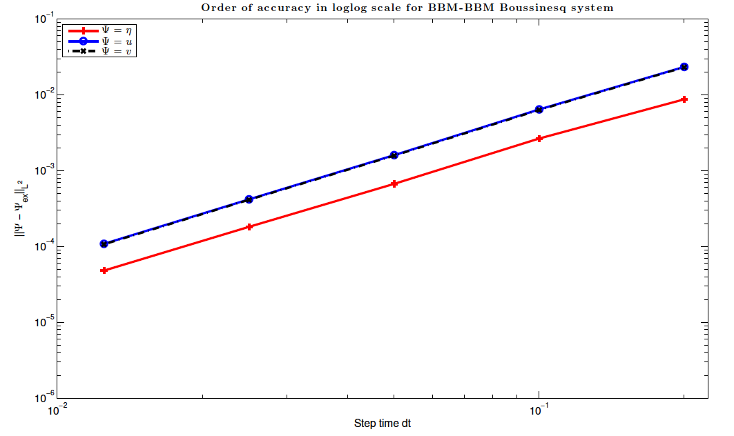
Figure 1: Rate of convergence for BBM-BBM.

4.3.2 Computation time

In this section, we consider the BBM-BBM Boussinesq system on the domain $\Omega=]-40,40[\times]-40,40[$ with $\mathbb{P}_{1}$ continuous piecewise linear functions, the space discretization $\Delta x=0.5$, the time step $\Delta t=0.1$ and as initial data $\eta_{h0}(x,y)=0.2e^{-(x^{2}+y^{2})/5},u_{h0}(x,y)=v_{h0}(x,y)=0$ with zero Dirichlet homogenous Boundary Conditions for $\eta_{h}$, $u_{h}$ and $v_{h}$ on the whole boundary.
In order to solve this system, we will show the time comparison of different method:

• M1 to solve Algorithm 1 without using adaptmesh technique and the keyword init.

• M1init to solve Algorithm 1 using the keyword init and without using adaptmesh technique.

• M1A-4 to solve Algorithm 1 using adaptmesh technique with err=1e-4 and without the keyword init.

• M1A-2 to solve Algorithm 1 using adaptmesh technique with err=1e-2 and without the keyword init.

• M2 to solve Algorithm 2 without using adaptmesh technique and the keyword init.

• M2init to solve Algorithm 2 using the keyword init and without using adaptmesh technique.

• M2A-4 to solve Algorithm 2 using adaptmesh technique with err=1e-4 and without the keyword init.

• M2A-2 to solve Algorithm 2 using adaptmesh technique with err=1e-2 and without the keyword init.

We present in Table 3, the time of computation in second at time $T=10s$ using all the different method cited before. All computation was made on a Macbook OS X, Intel core 2 Duo (CPU), 4Go (Memory), 2 Ghz (Processor).

M1	M1init	M1A-4	M1A-2
1555.48	722.507	115.485	45.3462
M2	M2init	M2A-4	M2A-2
1217.01	619.462	99.5689	39.3365

Table 3: Comparison of computation time for the different method used to solve the BBM-BBM system.

We note that, without using the mesh adaptation technique, we have the same result for all the computed solution, so we can see from Table 3 that the best method to use is the M2init.

In other hand, using the mesh adaptation technique, we can remark from Table 3 that the computation time is better then other method, but unfortunately, we have a little difference between the computed solution, that we plot in Figure 2 the square of $L^{2}$ norm of the error between the computed solution using the M1 method and the one computed with the M1A-8, M1A-6, M1A-4, M1A-2 methods where we have err=1e-8, err=1e-6, err=1e-4, err=1e-2, respectively vs the time till $T=30s$. We also plot in Figure 3 the mean of all the square of $L^{2}$ norm of the error computed for different mesh adaptation method.

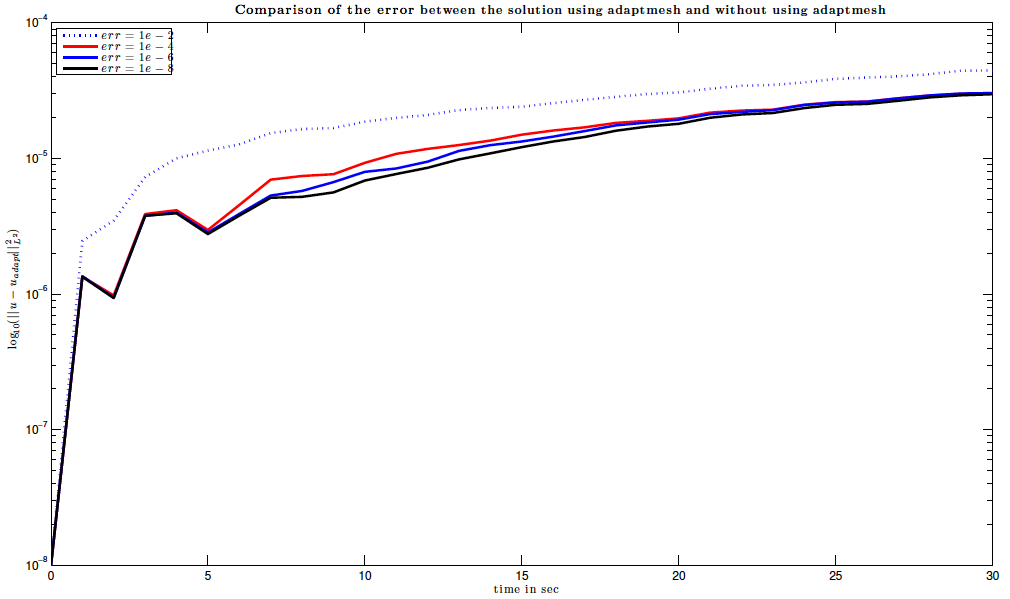
Figure 2: Comparison of the error between the solutions.

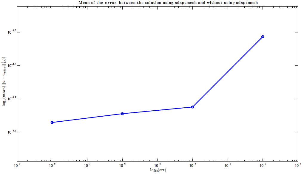
Figure 3: Mean of the error between the solutions.

We can remark from this result that we have the same result using M1A-8, M1A-6, M1A-4 method and the mean error between the solution computed with these method and the computed one using the M1 is of order $10^{-5}$ and we can see the large time difference.

4.3.3 Reflection of expanding symmetric waves at two boundaries of the BBM-BBM Boussinesq system

In Figures 4 and 5 we show the reflection from two parts of the boundary of an expanding symmetric wave of the BBM-BBM Boussinesq system where $a=c=0$ and $b=d=1/6$. For this experiment we used as initial data the functions $\eta_{h0}(x,y)=.2e^{-(x^{2}+y^{2})/5},u_{h0}(x,y)=v_{h0}(x,y)=0$. We used zero Neumann Boundary Conditions for $\eta_{h}$ on the whole boundary, zero Dirichlet data for $u_{h}$ and $v_{h}$ on $x=-40$ and $y=40$ (where we have the wall), and zero Neumann boundary data for $u_{h}$ and $v_{h}$ on $x=40$ and $y=-40$. The expanding waves are reflected from the $x=-40$ and $y=40$ parts of the boundary.
We note that in Figure 4 we show the effect of the mesh adaptation following the evolution of $\eta_{h}$ in time and in Figure 5 we show the propagation of the solution $\eta_{h}$.

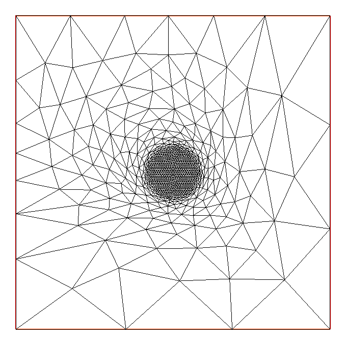
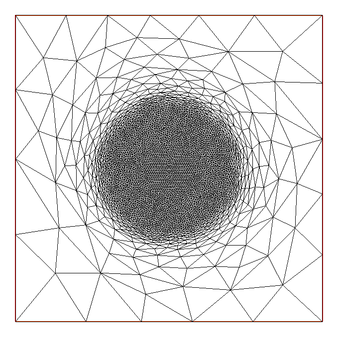
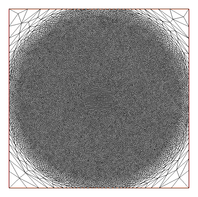
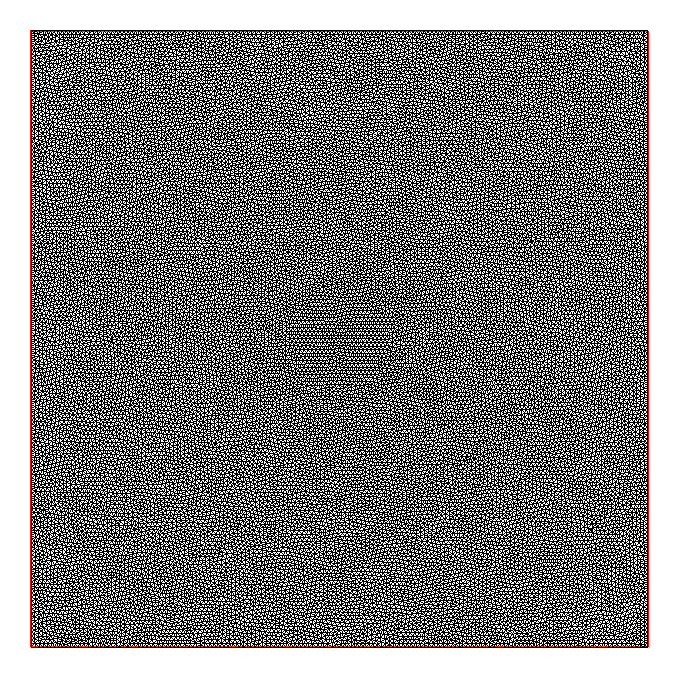
Figure 4: Propagation of the mesh for the BBM-BBM Boussinesq system where $a=c=0$ and $b=d=1/6$ for different time $t=\{0.1,20,40,70\}$

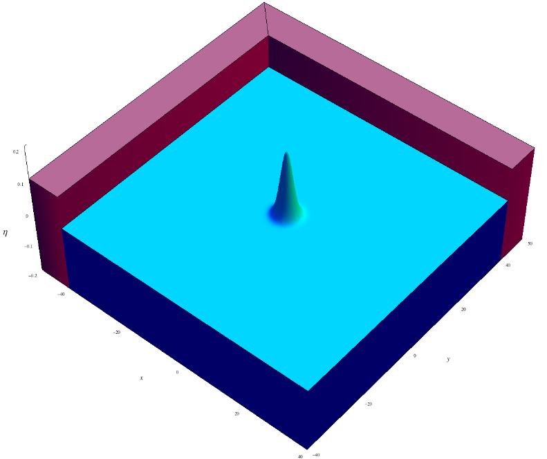
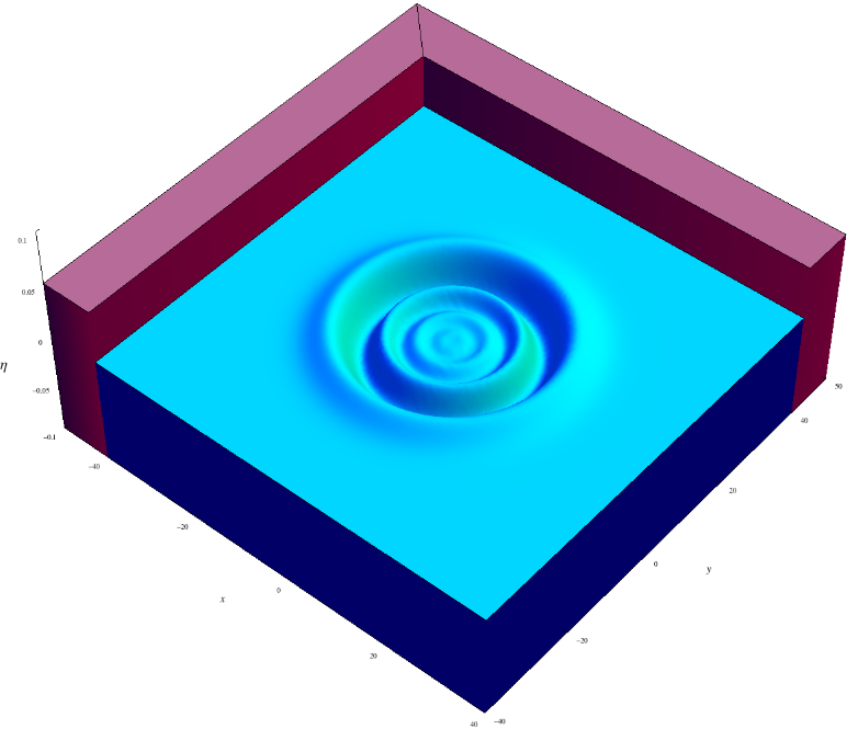
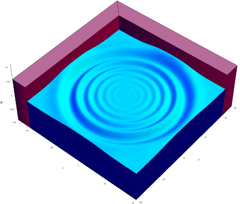
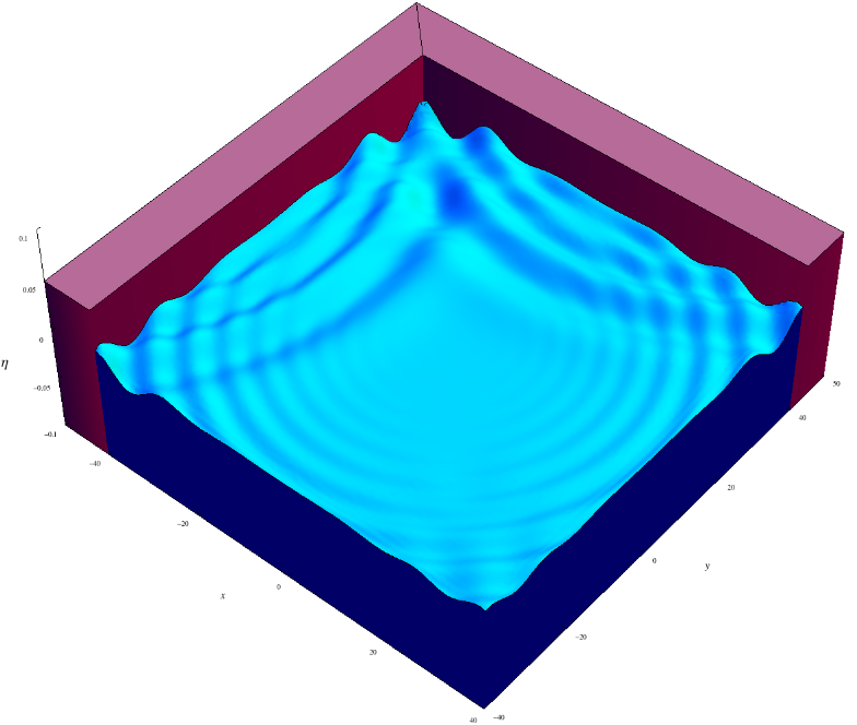
Figure 5: Propagation of the solution of the BBM-BBM Boussinesq system where $a=c=0$ and $b=d=1/6$ for different time $t=\{0,20,40,70\}$

4.3.4 Expanding symmetric waves under the KdV-KdV Boussinesq system

In Figure 6, we present the evolution of the $\eta_{h}$ profile emanating from the radially symmetric initial data $\eta_{h0}(x,y)=.5e^{-(x^{2}+y^{2})/5},u_{h0}(x,y)=v_{h0}(x,y)=0$, under the KdV-KdV Boussinesq system where $a=c=1/6$ and $b=d=0$. We used Bi-Periodic Boundary Conditions for $\eta_{h}$, $u_{h}$ and $v_{h}$ and we work with the time step $\Delta t=0.001$. We remark here that with these Bi-Periodic Boundary Conditions for $\eta$, $u$ and $v$ and their derivatives, in addition by integrating the equations in the system (2.1) on the hole domaine, we deduce the following mass conservation: $(Id-b\Delta)\displaystyle\int_{\Omega}\eta_{t}=0$ and the relations $(Id-d\Delta)\displaystyle\int_{\Omega}u_{t}=0$, $(Id-d\Delta)\displaystyle\int_{\Omega}v_{t}=0$. Hence:

$$\int_{\Omega}\eta=cte=\int_{\Omega}\eta_{0},\qquad\int_{\Omega}u=cte=\int_{\Omega}u_{0},\qquad\int_{\Omega}v=cte=\int_{\Omega}v_{0}.$$ (4.14)

In other hand, numerically, we see that these defined quantity are well conserved over time and we have:

$$\int_{\Omega}\eta=cte=\int_{\Omega}\eta_{0}=7.84527,\qquad\int_{\Omega}u=cte=\int_{\Omega}u_{0}=0,\qquad\int_{\Omega}v=cte=\int_{\Omega}v_{0}=0.$$

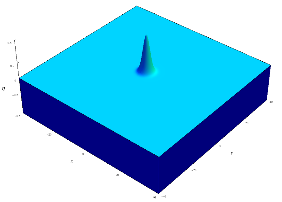
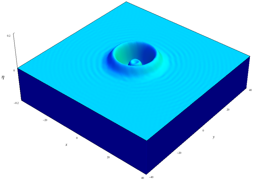
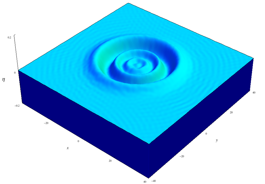
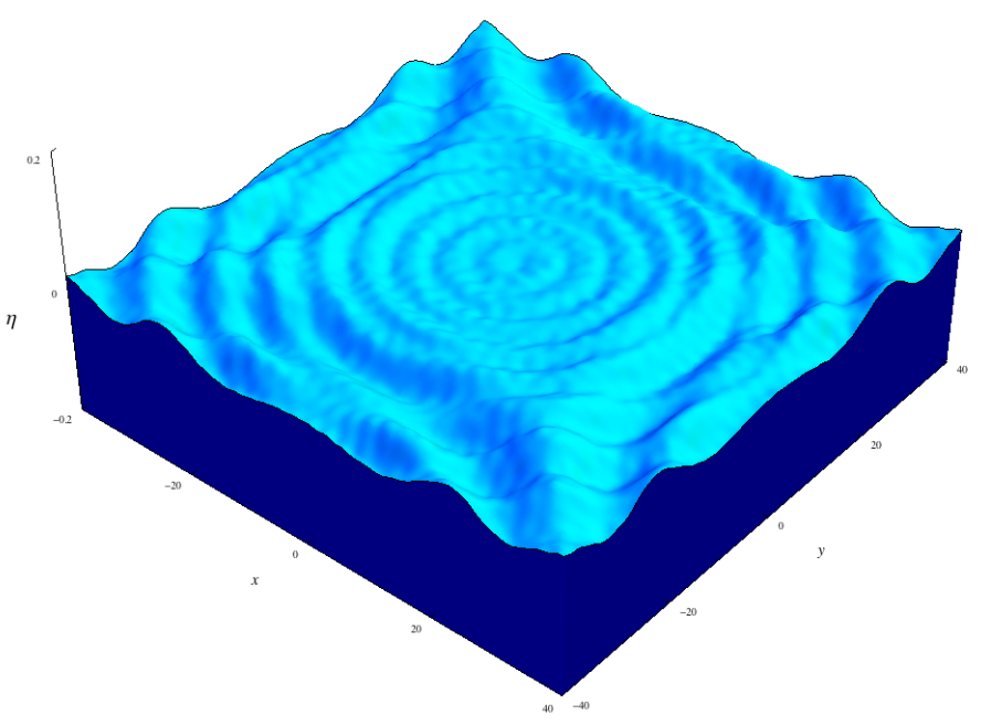
Figure 6: Propagation of the solution of the KdV-KdV Boussinesq system where $a=c=1/6$ and $b=d=0$ for different time $t=\{0,10,20,60\}$

We can see in Figure 6 from $t=10$ a small amplitude periodic profile (ripples) which are propagating in front of the wavefront and which has been observed in [4] (in the case of 1D KdV-KdV system). These ripples are still observed when using $\mathbb{P}_{2}$ elements but they do not infer to the numerical stability, we still have the mass conservation of the fluid.

Other simulation for different Boussinesq systems can be found in [18].

4.4 Comparison of the results with Mitsotakis et al.

We validate also our code by comparing the results with those of Mitsotakis et al. [9] (in Figure 8, page 847) where they consider the cross section in $x$ direction to the $\eta$ component of the solution from radially symmetric initial data of the form $\eta_{h0}(x,y)=.2e^{-(x^{2}+y^{2})/5}$ with $u_{h0}(x,y)=v_{h0}(x,y)=0$ under the BBM-BBM and the Bona-Smith system, both considered with zero Dirichlet boundary conditions for $\eta,u$ and $v$. We remark in Figure 7, that the shape of the solution for the results of our code at the left part and for those of Mitsotakis et al. code at the right part are similar.
We note also that in their paper, they used Galerkin finite elements based on tensor products of smooth splines and an explicit second order (for BBM-BBM system with bilinear splines) and fourth order (for Bona-Smith system with bi-cubic splines) Runge-Kutta scheme while in the present work, we used $\mathbb{P}_{1}$ continuous piecewise linear functions and an explicit second order Runge-Kutta scheme for all systems.

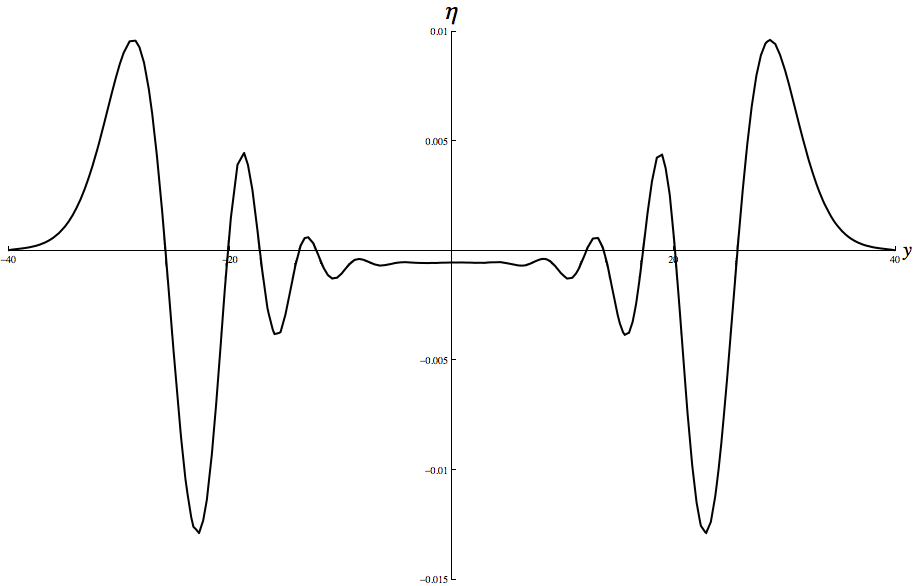
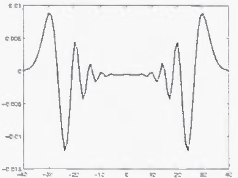
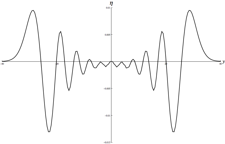
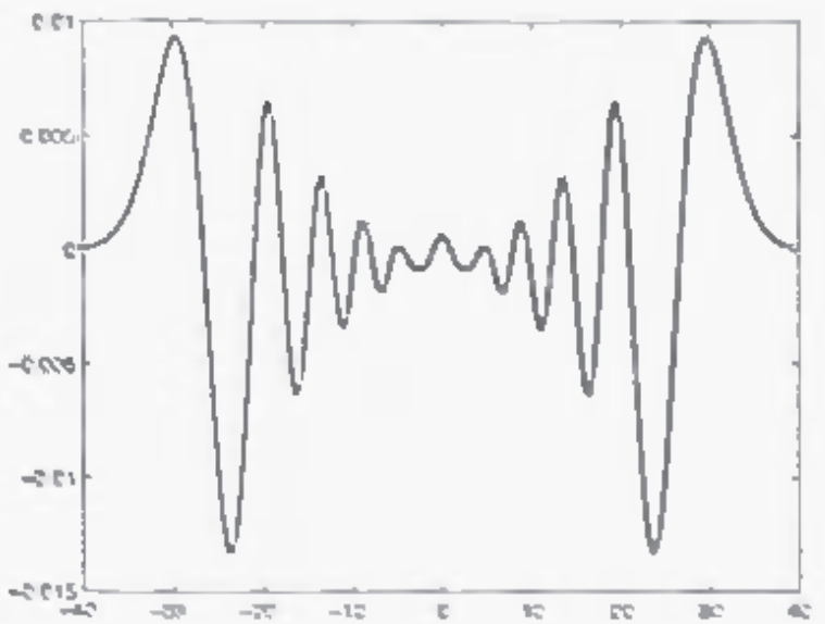
Figure 7: Cross sections in $x$ direction of $\eta(x,y,t)$ at $t=30s$, Bona-Smith (above) and BBM-BBM (below), using our code (left) and Mitsotakis et al. code (right) borrowed from the article [9].

4.5 Comparison of different Boussinesq models

We compare here KdV-KdV, BBM-BBM and Bona-Smith models as defined in section 2.1 Table 1.
In Figures 8, we present a comparison of the evolution of the $\eta$ component of the solution from radially symmetric initial data of the form $\eta_{h0}(x,y)=.5e^{-(x^{2}+y^{2})/5}$ with $u_{h0}(x,y)=v_{h0}(x,y)=0$, under the BBM-BBM (solid line with zero Dirichlet b.c., $\Delta t=0.1$, $\Delta x=0.5$), the Bona-Smith system (dotted line with zero Dirichlet b.c., $\Delta t=0.1$, $\Delta x=0.5$) and the KdV-KdV system (dashed line with periodic b.c., $\Delta t=0.001$, $\Delta x=0.5$). Figure 8 shows the cross sections of the $\eta$ profiles for different time in the $x$ - direction. The speed and the amplitude of the outgoing front is approximately the same for the BBM-BBM and Bona-Smith systems but the pattern of the oscillations behind the fronts are different: in the case of the Bona-Smith system the two outgoing wave trains have practically separated by $t=25s$, while the larger in amplitude dispersive oscillatory tails of the BBM-BBM solution seem to be still interacting. In other hand, the speed of the outgoing front for the KdV-KdV system is approximately the same with other systems while the amplitude for the internal crest is bigger, we remark also that the solution still interacting after $t=25s$.

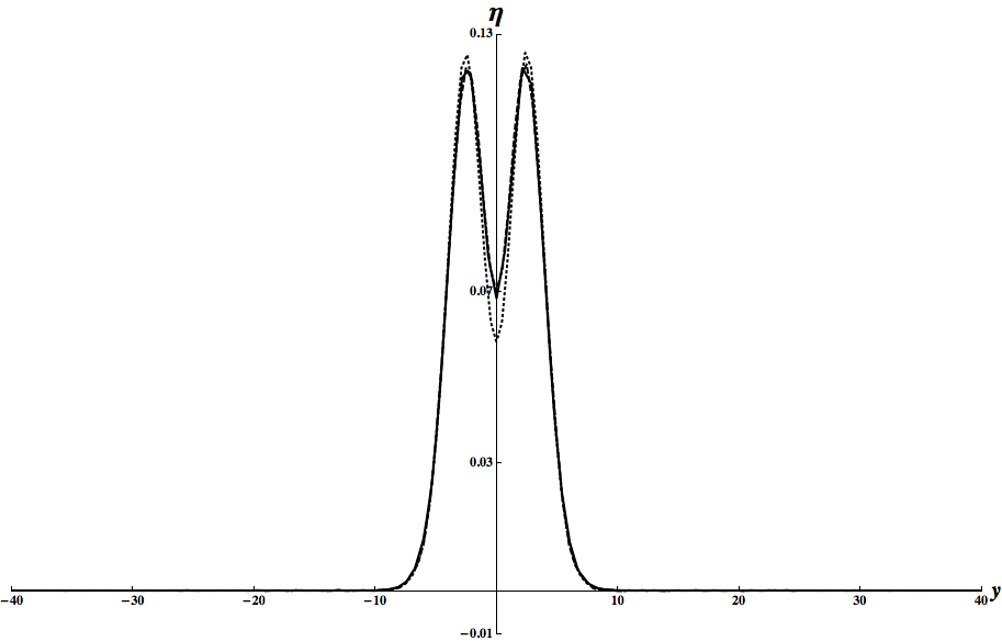
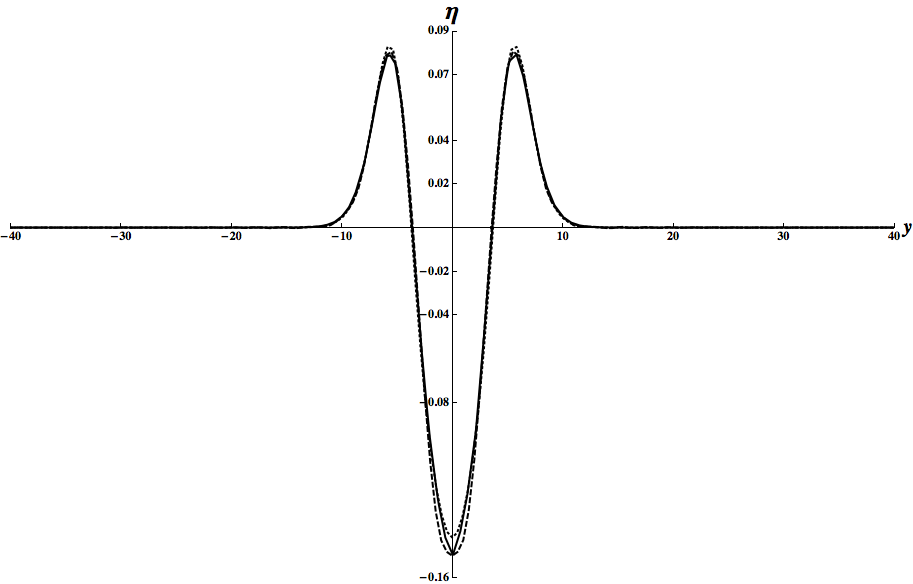
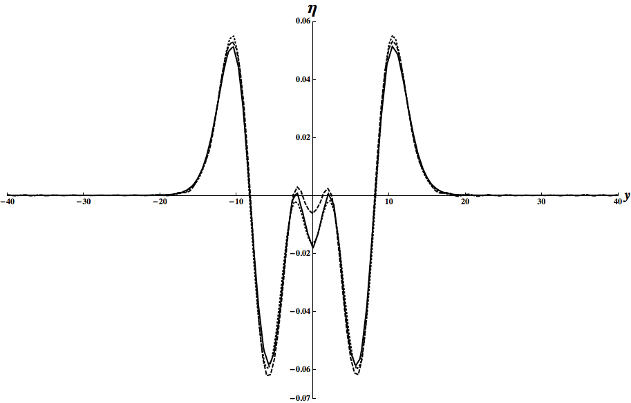
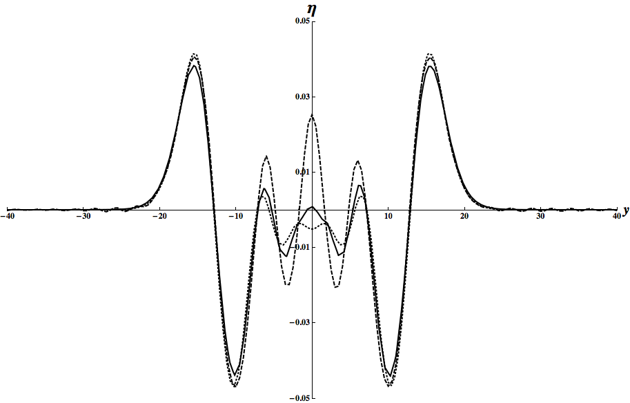
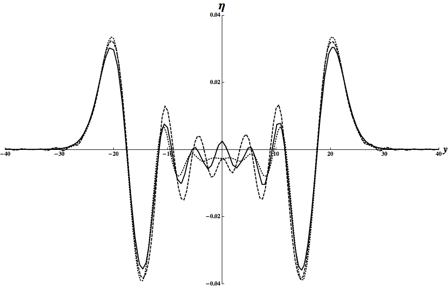
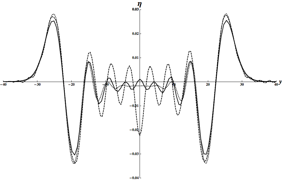
Figure 8: Comparison of the cross sections in $x$ direction of $\eta(x,y,t)$ at time $t=\{2,5,10,15,20,25\}s$, where in all the figure, the dotted line is for Bona-Smith system, the dashed for KdV-KdV one and the solid line for BBM-BBM one.

5 Conclusion

We have presented a numerical approach with # FreeFem ++ to solve the Boussinesq systems with a flat bottom, we validated our code and establishes the adequacy of the chosen finite element discretization by comparing the results with those of Mitsotakis et al. We have established also the feasibility of simulating complex equations of hydrodynamics as Boussinesq systems with # FreeFem ++ and we have optimized the algorithm that we use in section 4.3.2.
Using this approach, we can consider the case of a variable bottom (in space and/or in time), see [18] which is an ongoing work to appear soon. As a feature we address the simulation of Tsunamis with our approach, by including realistic data (bathymetry, generation of tsunami waves).
Acknowledgements: This work is supported by the regional program ”Appui à l émergence” of the Region Picardie. I would like to thank my PhD advisor Jean-Paul Chehab (LAMFA, Amiens), Denys Dutykh (LAMA, Savoie), Gloria Faccanoni (IMATH, Toulon), Kirill Pichon Gostaf (LJLL, Paris), Frédéric Hecht (LJLL, Paris), Antoine Le Hyaric (LJLL, Paris), Youcef Mammeri (LAMFA, Amiens), Olivier Pantz (CMAP, Paris) and Dimitrios Mitsotakis (IMA, University of Minnesota) for fruitful discussions and remarks.