The Dynamics of the Solar Radiative Zone

Abstract

The dynamics of the solar radiative interior are still poorly constrained by comparison to the convective zone. This disparity is even more marked when we attempt to derive meaningful temporal variations. Many data sets contain a small number of modes that are sensitive to the inner layers of the Sun, but we found that the estimates of their uncertainties are often inaccurate. As a result, these data sets allow us to obtain, at best, a low resolution estimate of the solar core rotation rate down to approximately $0.2{R_{\odot}}$. We present inferences based on mode determination resulting from an alternate peak-fitting methodology aimed at increasing the amount of observed modes that are sensitive to the radiative zone, while special care was taken in the determination of their uncertainties. This methodology has been applied to MDI and GONG data, for the whole Solar Cycle 23, and to the newly available HMI data. The numerical inversions of all these data sets result in the best inferences to date of the rotation in the radiative region. These results and the method used to obtain them are discussed. The resulting profiles are shown and analyzed, and the significance of the detected changes discussed.

1 Introduction

S-Introduction

Ground-based helioseismic observations (e.g. GONG: Harvey et al., 1996; BiSON: Broomhall et al., 2009) and space-based ones (e.g. MDI: Scherrer et al., 1995; GOLF: Gabriel et al., 1995; or HMI: Scherrer et al., 2012), have allowed us to derive a good description of the dynamics of the solar interior (e.g. Thompson et al., 2003, García et al., 2007, Eff-Darwich et al., 2002, 2008, Howe, 2009). Helioseismic inferences have confirmed that the differential rotation observed at the surface persists throughout the convection zone. The outer radiative zone ($0.3<{r/R_{\odot}}<0.7$) appears to rotate approximately as a solid body at an almost constant rate ($\approx 430$ nHz), whereas it is not possible to rule out a different rotation rate for the innermost core ($0.19<{r/R_{\odot}}<0.3$). At the base of the convection zone, a shear layer — known as the tachocline — separates the region of differential rotation throughout the convection zone from the one with rigid rotation in the radiative zone. Finally, there is a subsurface shear layer between the fastest-rotating layer, located at about $0.95{R_{\odot}}$, and the surface. Of course, this rotation profile is not constant; the time-varying component of the rotation displays clear variations near the surface (known as the torsional oscillations), while we see hints of variations at the base of the convection zone, both being likely related to the driving mechanisms of the solar-activity cycle.

Our understanding of the dynamics of the solar interior has undoubtedly improved; however we still need to constrain the rotation profile near the core and fully analyze the nature of the torsional oscillations. We still do not know how thin the tachocline really is and what is keeping it this way. Understanding the tachocline should help discern if there is a fossil magnetic field in the radiative zone that prevents the spread of the tachocline (Zahn et al., 2007), or an oscillating magnetic field (Forgács-Dajka and Petrovay, 2001). No purely fluid-dynamics mechanism can explain the tachocline, resulting in a compelling argument for the presence of a strong magnetic field (Gough and McIntyre, 1998).

The proper knowledge of the relationship between the solar dynamics and its structure is not important only in order to understand the present conditions of the Sun, but also to understand the temporal evolution of our star and other solar-like stars. It is usually assumed that the main characteristics of the dynamics of the Sun were established during its contraction phase (Turck-Chièze et al., 2010), hence the Sun was not a rapid rotator when it entered the Zero Age Main Sequence (ZAMS). The transport of momentum during the contraction phase might have been carried out by a magnetic field in the core and the diffusion of this field flattened the rotation profile in the rest of the radiative zone (Duez et al., 2010). In any case, theories about the mechanisms that drive the solar rotation and its spatial and temporal variations remain to be tightly constrained by improved helioseismic inversion results. Better rotation profiles mean not only improved inversion methodologies but improved estimates of rotational-frequency splittings.

We present here results derived using an improved inversion methodology that i) adjusts the inversion grid (over both depth and latitude) based on the data set and its precision, and ii) solves the inversion problem iteratively. But first we review recent developments in global mode characterization (Korzennik, 2008) that allowed us to infer with better confidence the internal-rotation rate and its time varying patterns. We describe in detail the inversion methodology and show the resulting profiles.

2 The Data Sets

2.1 Introduction

We have used rotational frequency splittings determined from fitting data acquired with five different instruments. Two are ground based: the Birmingham Solar Oscillations Network (BiSON) and the Global Oscillation Network Group (GONG) and three are on-board spacecraft: the Global Oscillations at Low Frequencies (GOLF) and the Michelson Doppler Imager (MDI) on board the Solar and Heliospheric Observatory (SOHO), and the Helioseismic and Magnetic Imager (HMI) on board the Solar Dynamics Observatory (SDO). For all but the last instrument, the available data sets span well over a decade of observations. Table tab:datasets summarizes what data, from which instrument, and for what time span are included in this study.

Instrument	Time span
BiSON (ground-based)	01 Jan 1992 – 31 Dec 2002
GONG (ground-based)	07 May 1995 – 11 Feb 2011
GOLF (SOHO)	21 May 1996 – 07 Jun 2007
MDI (SOHO)	01 May 1996 – 12 Dec 2008
HMI (SDO)	30 Apr 2010 – 16 Sep 2011

Table 1.: List of instruments and time span from which data sets were used in the work presented here.tab:datasets

The data from these five instruments were fitted with various techniques, and in some cases the same data were fitted with more than one methodology. The GOLF and BiSON data were fitted, using “Sun-as-a-star” fitting techniques, as described by Garcia et al. (2008) and Broomhall et al. (2009), respectively. The fitting, in both cases, is limited by these instruments’ lack of spatial resolution to low degree modes ($\ell\leq 3$).

The methodology for the mode fitting pipeline used by the GONG project is described by Anderson et al. (1990). It processes 108-day long overlapping time series, each 36 days apart, and individually fits each multiplet. It does it without including any spatial leakage matrix information and uses a symmetric profile for the mode power-spectral density. When resolved, spatial leaks are independently fitted, but when they are not resolved (in most cases), blended leaks are fitted as a single peak. Since there is no inclusion of any leakage information, the blending affects the result, skewing the mode frequency and the mode line width.

The mode-fitting pipelines used by the MDI team (both the standard and “improved” pipelines) fit non-overlapping 72-day long epochs. That fitting methodology fits singlets, using a polynomial expansion in $m$ to model the frequency splitting, and includes the leakage matrix information (as described by Schou, 1992). The improved pipeline (Larson and Schou, 2008) includes an improved spatial decomposition, where the effective instrument plate scale and our best model of the image distortion is included, as well as an improved leakage computation that incorporates the distortion of the eigenmodes by differential rotation (Woodard, 1989). The improved pipeline is set up to fit either a symmetric or an asymmetric mode power spectral density profile.

2.2 Our Alternate Peak-Fitting Method

Korzennik (2005, 2008) has developed and implemented an alternative fitting methodology, which has processed GONG, MDI, and HMI data. The key elements of this method are as follow: it fits individual multiplets, simultaneously for all the azimuthal orders while including the leakage information. The leakage matrix includes the effect of the distortion of the eigenmodes by differential rotation (Woodard, 1989). The spectral estimator is a sine multi-tapered one, whose number of tapers is adjusted to be optimal, a value derived from the mode line-width. The mode power-spectral density profile is asymmetric, the procedure is iterative so as to include mode contamination (mode with a different radial order [$n$] present in the fitting window), and it includes a rejection factor, where modes with too low an amplitude are not fitted.

The other major difference in the implementation of this method is that we choose to fit time series of varying lengths. The gain in signal-to-noise ratio when using longer time series allows us to derive more accurate mode parameters, while trading off precision for temporal resolution. We used $64\times,32\times,16\times,8\times,4\times$ and $2\times 72$-day long, overlapping, time-series, as well as $1\times 72$-day long non-overlapping epochs (note that the longer segments all start on 01 May 1996, i.e. the start of science quality observations for MDI). This extensive analysis of some 13 years of data was carried out on the Smithsonian Institution High Performance Cluster.

This method was used to fit GONG time series, using a leakage matrix specifically computed for that instrument, although the change in leakage resulting from the 2001 camera upgrade was not yet included (Schou, private communication, 2003). That same method was used to fit MDI data, for the exact same epochs, but using an MDI-specific leakage matrix. In fact, we fitted the data using a leakage matrix supplied by the MDI team, as well as our own independent leakage matrix computation. We used the “improved” MDI time series, where the spatial decomposition includes the effective instrument plate scale and our best model of the image distortion. We also fitted HMI provisional time series (as the HMI processing pipeline is yet to be finalized). The HMI instrumental image distortion and precise plate scale are included at the filtergram processing level, and the data were fitted using a provisional leakage matrix (i.e. the one derived for the full-disk MDI observations).

Figures fig:compare-freqs and fig:compare-cgs-1 and Table tab:compare-cgs compare results from fitting GONG and MDI data with the respective projects analysis pipelines and the above described alternate fitting method. The table lists the mean and standard deviation of the differences in the $a_{1}$ Clebsch–Gordan coefficients (linear term) estimated by various fitting procedures. The resulting singlets show systematic differences, that are not simply explained by the inclusion or not of an asymmetric profile, with even larger and systematic differences for the f-mode. The comparisons of the rotational-splitting coefficients show less of a scatter for the linear term, when using the alternate peak-fitting method, and differences at the few $\sigma$ level.

But also, if not more important, is the difference in mode attrition, when using the various fitting methods. Figure fig:show-attrition illustrates that mode attrition, i.e. how often a mode is successfully fitted for each epoch analyzed. That figure shows clearly that the project pipeline methods produce large attrition, while the alternate peak-fitting method results display a more consistent fitting pattern. In order to be confident that we deduce significant changes of the solar rotation, when inverting rotational frequency splittings for various epochs, we ought not to inject changes resulting from using different mode sets in the inversions. The estimated solutions of an inversion problem are some weighted spatial average of the “real” underlying solution. Those weights (also known as resolution kernels) depend on the extent of the input set, and thus change when the input sets change.

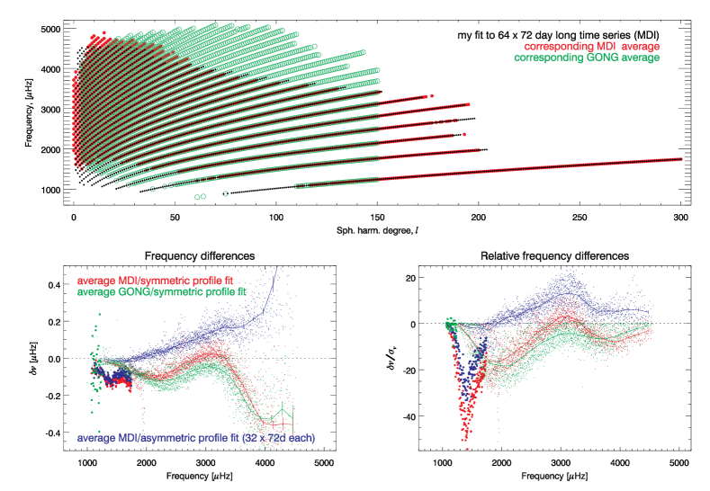
Figure 1.: Comparison of fitted frequencies (singlets): top panel shows the coverage in the $\ell-\nu$ plane, bottom panels shows frequency and relative frequency differences (i.e., differences divided by the uncertainty), relative to the alternate fitting methodology. Black dots correspond to modes fitted using the alternate fitting methodology, applied to $64\times 72$-day long time series, the red and green dots correspond to MDI and GONG pipeline fitting respectively, while the blue dots correspond to MDI “improved” fitting, using an asymmetric profile. The large dots correspond to the f-modes, the curves are the p-mode corresponding binned values.fig:compare-freqs

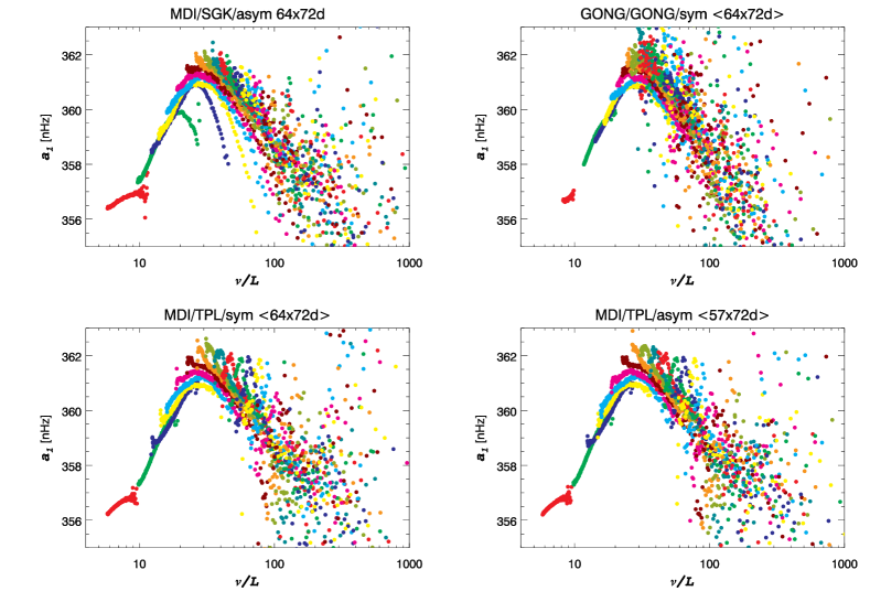
Figure 2.: Comparison of the frequency splitting leading Clebsch–Gordan coefficient derived from four mode-fitting procedures: (a) results from using our alternative fitting methodology, (b) GONG pipeline, (c) MDI improved symmetric fit, and (d) MDI improved asymmetric fit. The resultiong $a_{1}$ coefficients are plotted versus $\frac{\nu}{L}$, where $L^{2}=\ell(\ell+1)$, while the symbol’s color corresponds to the mode order, $n$.fig:compare-cgs-1

	$\delta a_{1}$	$\delta a_{1}/\sigma_{a_{1}}$
	[nHz]
GONG (sym.) vs alternate (asym.) $64\times 72$-day long	$-0.277\pm 0.984$	$-0.917\pm 1.279$
MDI (sym,) vs alternate (asym.) $64\times 72$-day long	$0.051\pm 0.635$	$0.534\pm 2.888$
MDI (asym.) vs alternate (asym.) $32\times 72$-day long	$0.096\pm 0.769$	$1.398\pm 2.384$

Table 2.: Comparison of resulting $a_{1}$ Clebsch–Gordan coefficients (linear term) derived from four mode fitting procedures. The table lists the mean and standard deviation of the differences in $a_{1}$.tab:compare-cgs

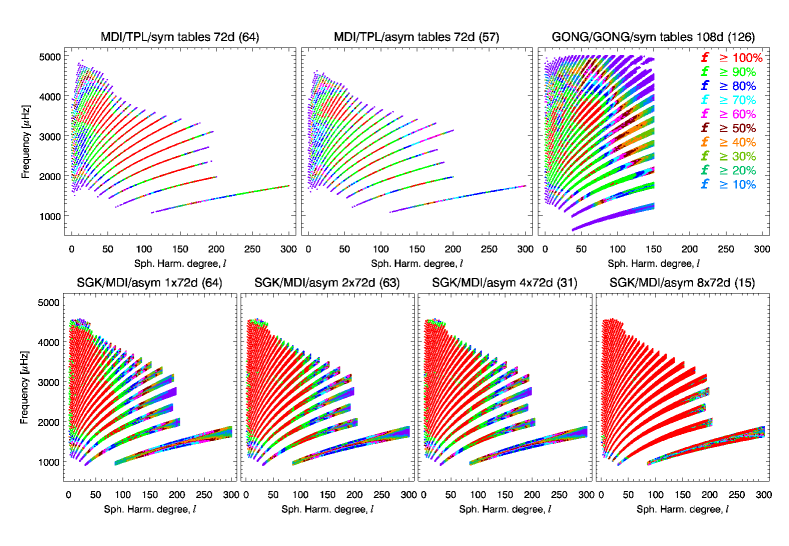
Figure 3.: Mode attrition in the $\ell-\nu$ plane. The color represents how often a mode is fitted, with red indicating all the time ($f=100\%$), green 90%, etc. The top panels correspond to MDI improved symmetric and asymmetric fit and GONG pipeline fit. The bottom panels correspond to our alternative fitting methodology, for $1\times$, $2\times$, $4\times$, $8\times 72$-day long time series (left to right).fig:show-attrition

3 Inversion Methodology

The starting point of all helioseismic, linear rotational inversion methodologies is the functional form of the perturbation in frequency [$\Delta\nu_{n\ell m}$] induced by the rotation of the Sun, $\Omega(r,\theta)$:

$$\Delta\nu_{n\ell m}=\int_{0}^{{R_{\odot}}}\!\!\!\!\int_{0}^{\pi}\!\!K_{n\ell m}(r,\theta)\,\Omega(r,\theta)\,\mathrm{d}r\,\mathrm{d}\theta\pm\epsilon_{n\ell m}\ilabel{eq:equation1}$$ (1)

The perturbation in frequency [$\Delta\nu_{n\ell m}$] with the observational error [$\epsilon_{n\ell m}$] that corresponds to the rotational component of the frequency splittings, is given by the integral of the product of a sensitivity function, or kernel [$K_{n\ell m}(r,\theta)$] with the rotation rate [$\Omega(r,\theta)$] over the radius [$r$] and the co-latitude [$\theta$]. The kernels [$K_{n\ell m}(r,\theta)$] are known functions of the solar model.

Equation (eq:equation1) defines a classical inverse problem for the Sun’s rotation. The inversion of this set of $M$ integral equations – one for each measured $\Delta\nu_{n\ell m}$ – allows us to infer the rotation rate profile as a function of radius and latitude from a set of observed rotational frequency splittings (hereafter referred as splittings).

Our inversion method requires the discretization of the integral relation to be inverted. In our case, Equation (eq:equation1) is transformed into a matrix relation

$$D=Ax+\epsilon\ilabel{eq:equation2}$$ (2)

where $D$ is the data vector, with elements $\Delta\nu_{n\ell m}$ and dimension $M$, $x$ is the solution vector to be determined at $N$ model grid points, $A$ is the matrix with the kernels of dimension $M\times N$, and $\epsilon$ is the vector containing the corresponding observational uncertainties. The number and location of the $N$ model grid nodes are calculated according to the effective spatial resolution of the inverted data set. Such a procedure produces a non-equally spaced (i.e.  unstructured) mesh distribution. A complete description and examples of the gridding methodology can be found in Eff-Darwich and Pérez-Hernández (1997) and Eff-Darwich et al. (2010).

The resulting unstructured grid is used to compute the matrix $A$ in Equation (eq:equation2). That equation is then solved with a modified version of the iterative method developed by Starostenko and Zavorotko (1996). This approach calculates $x$ according to the following algorithm:

$$x^{k+1}=x^{k}-B^{-1}A^{T}R^{-1}(Ax^{k}-D)$$ (3)

where $k$ is the iteration index. The diagonal matrices $B$ and $R$ are calculated from the summation of columns and rows of matrix $A$, respectively. For each iteration, values for the error propagation and data misfit, $\chi^{2}=|Ax-D|^{2}$, are calculated.

4 Results

Helioseismology, as a tool to infer the properties of the solar interior, is based on the fact that different mode sets are sensitive to different layers of the Sun. Hence, by combining these mode sets, it is possible to derive the structure and dynamics of the solar interior. However, these sets are not homogeneous and the number and quality of the modes that are sensitive to the solar radiative interior is significantly lower than those sensitive to the convective zone and the surface layers (as shown in Figure fig:0). Therefore, the dispersion and the level of uncertainties of the modes that are sensitive to the core are the largest for the entire data set. Another problem arises as we look closely at the uncertainties (see Figure fig:0): the error level as a function of radius is not strictly monotonic. For a given inner turning radius, the scatter of the errors is rather large, and is primarily the consequence of the reduced accuracy of estimates at high frequencies.

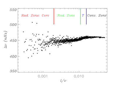
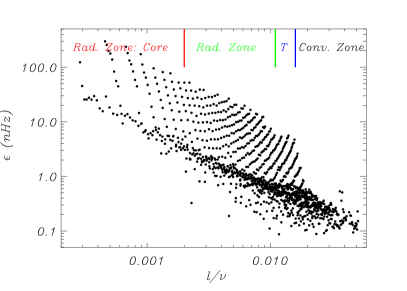
Figure 4.: Left panel: observational sectoral frequency splittings (MDI $64\times 72$-day long time series) as a function of the $\frac{\ell}{\nu}$ ratio, a proxy for the inner turning radius. For illustrative purposes, the approximate extent of the solar core, radiative zone, tachocline and convective zone are represented. Right panel: as in the left panel, but for the observational uncertainties of sectoral frequency splittings. fig:0

Figure fig:17 shows how consistent both the range in degree and frequency are when the alternative fitting technique developed for this work is used on data from different instruments. By contrast, the mode sets obtained by the team pipelines, for both GONG and MDI, differ significantly, especially for their frequency spans. The consistency of our fitting technique is shown in Figure fig:15: this figure shows how both the uncertainties and the data dispersion are reduced when the length of the time series analyzed is increased. The improvement is less apparent for the modes that are more sensitive to the solar core and in the data sets corresponding to shorter time-series. However, in the case of the $64\times 72$-day long mode set, the uncertainties for the modes sensitive to the core are reduced by a factor of four relative to the mode sets obtained from shorter time series.

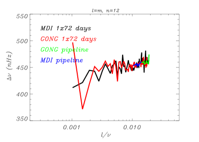
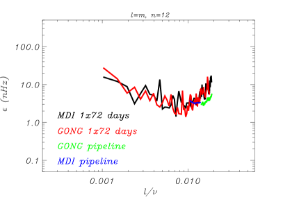
Figure 5.: Left panel: observational sectoral frequency splittings as a function of the $\frac{\ell}{\nu}$ ratio, a proxy for the inner turning radius, for $n=12$ modes obtained by fitting MDI $1\times 72$, GONG $1\times 72$-day long time-series and the MDI and GONG team pipelines. Right panel: as in the left panel, but for the observational uncertainties. fig:17

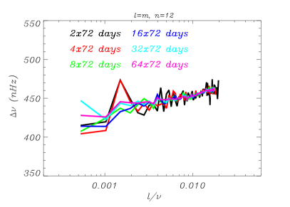
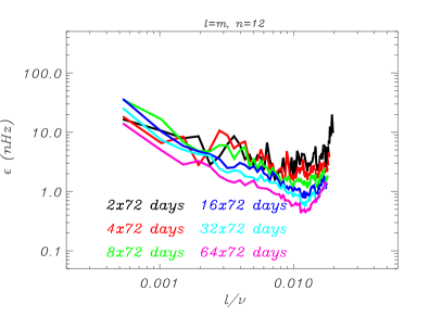
Figure 6.: Left panel: observational sectoral frequency splittings as a function of the $\frac{\ell}{\nu}$ ratio, a proxy for the inner turning radius, for $n=12$ modes obtained by fitting MDI $2\times$, $4\times$, $8\times$, $16\times$, $32\times$, and $64\times 72$-day long time-series. Right panel: as in the left panel, but for the observational uncertainties. fig:15

Hence, uncertainties of the data sensitive to the solar core rotation decrease when longer time-series and better fitting technique are used. The level of uncertainties that we need to reach to counteract the low sensitivity of the modes to these regions is illustrated in Figure fig:3, with test profiles. Two sets are presented: i) one set where the radiative zone is rotating rigidly, at a rate of $432$ nHz, and below $0.12R_{\odot}$ at rates of $2832$, $835$, and $132$ nHz; ii) the other set where the radiative zone is also rotating rigidly at a rate of $432$ nHz, and where below $0.2R_{\odot}$ the rates are again set to $2832$, $835$, and $132$ nHz. Out of these six test profiles, only one is substantially and significantly different from the frequency-averaged $\ell=1$ rotational splittings (i.e.  averaged over frequencies in the 1.1 to 3.3 mHz range) derived from our peak-fitting methodology (MDI and GONG $64\times 72$ days), the MDI pipeline (using a 2088-day long time series), GOLF, and BiSON data sets.

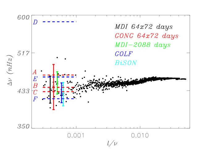
Figure 7.: Observational sectoral frequency splittings as a function of the horizontal phase speed for $\ell=1$ modes (MDI $64\times 72$-day long time series). The vertical colored lines represent the frequency-averaged (1.1to 3.3 mHz) $\ell=1$ rotational splittings derived from our peak-fitting methodology (MDI and GONG $64\times 72$ days), the MDI pipeline (using a 2088-day long time series), GOLF and BiSON.The red dashed lines represent the average values of the theoretical $\ell=1$ rotational splittings, if the radiative zone were rotating rigidly at a rate of $432$ nHz, with rates below $0.12R_{\odot}$ of $2832$, $835$, and $132$ nHz (A, B and C respectively). The blue dashed lines represent the average values of the theoretical $\ell=1$ rotational splittings, with rates below $0.2R_{\odot}$ of $2832$, $835$, and $132$ nHz (D, E and F respectively). fig:3

The diagnostic potential of the new global-mode fitting technique when combined with the improved inversion methodology is illustrated in Figures fig:27, fig:28, and fig:30, where we present the time-averaged rotation profiles of the Sun from the surface down to $0.15{R_{\odot}}$ that were calculated, using either MDI or GONG, and $2\times$, $4\times$, $8\times$, $16\times$, $32\times$, and $64\times 72$-day long time-series. Inversions using recent HMI data ($2\times$ and $4\times 72$-day long) are also presented, although they are not yet comparable to either MDI or GONG results, since the amount of HMI observations is still significantly smaller.

Both MDI and GONG inversions give similar results, with the largest discrepancies at high latitudes and below $0.40R_{\odot}$. The most significant difference between the inversions obtained by the same instrument is the reduction of the uncertainties, in particular random noise, when the length of the time-series used to fit is increased. This reduction is particularly important in the inner radiative core.

All results are compatible with a radiative zone rotating rigidly at a rate of approximately 431 nHz; however, it is not possible to disregard a faster or slower rotator below $0.2{R_{\odot}}$ (i.e.  up to 600 or down to 300 nHz). Although the radiative zone seems to rotate rigidly, there is a consistent and systematic dip in the rotation profile located at approximately $0.4{R_{\odot}}$ and $60^{\rm o}$ in latitude. This dip is seen in both MDI and GONG results, notwithstanding the actual length of the fitted time series.

This result is intriguing, particularly if we analyze the time evolution of the dip, for both MDI and GONG derived profiles, as shown in Figure fig:35. It was not possible to include the $1\times$ and $2\times 72$-day long results, since the quality of the inverted profiles at that depth and latitude is too low. Therefore, we used the $4\times 72$-day long data, since its precision and temporal resolution allow us to carry out a temporal evolution analysis with adequate quality of the resulting profiles. Although the dip is certainly at the limit of the resolution of the data and the inversion method, there is a systematic temporal change of the dip. This variation is not found at other latitudes.

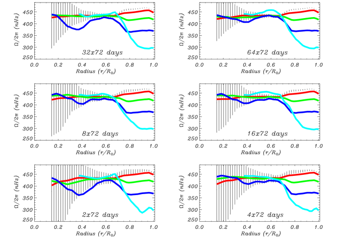
Figure 8.: Time-averaged rotational profiles obtained from the inversions of rotational frequency-slittings resulting from fitting MDI $2\times$, $4\times$, $8\times$, $16\times$, $32\times$, and $64\times 72$-day long time-series. Black, red, green, dark-blue, and light-blue lines correspond to the rotational rate at different latitudes, namely $0,20,40,60$, and $80^{\rm o}$, respectively. Vertical lines represent the error bars for the rotational rate at the Equator.fig:27

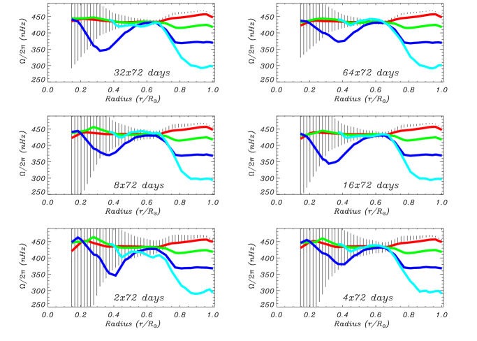
Figure 9.: Time-averaged rotational profiles obtained from the inversions of rotational frequency-slittings resulting from fitting GONG $2\times$, $4\times$, $8\times$, $16\times$, $32\times$, and $64\times 72$-day long time-series. Black, red, green, dark-blue, and light-blue lines correspond to the rotational rate at different latitudes, namely $0,20,40,60$, and $80^{\rm o}$, respectively. Vertical lines represent the error bars for the rotational rate at the Equatorfig:28

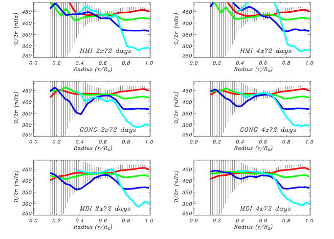
Figure 10.: Time-averaged rotational profiles obtained from the inversions of MDI, GONG, and HMI $2\times 72$ and $4\times 72$-day long sets. Black, red, green, dark-blue, and light-blue lines correspond to the rotational rate at different latitudes, namely $0,20,40,60$, and $80^{\rm o}$, respectively. Vertical lines represent the error bars for the rotational rate at the Equator.fig:30

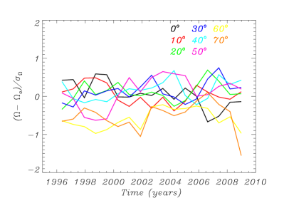
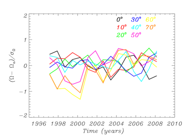
Figure 11.: Left panel: temporal evolution of the relative residual rotation rate, $(\Omega-\Omega_{o})/\sigma_{\Omega}$, where $\Omega_{o}/2\pi=432$ nHz, at a depth of $0.4{R_{\odot}}$ and for different latitudes obtained from the inversion of the different MDI $4\times 72$-day long data sets. Right panel: as in the left panel, but for GONG data. fig:35

The consequences of using different peak fitting techniques on the inversion results is illustrated in Figure fig:29. That figure shows the time-averaged rotational rates obtained using MDI and GONG $2\times 72$-day long alternative fitting method and GONG and MDI respective project pipelines. The lengths of the fitted time-series are comparable, however the spherical harmonic degree and frequency ranges of the fitted mode sets differ significantly. In particular, the mode sets obtained by the project pipelines result in rotational profiles that significantly disagree in the spatial extent of the optimal inversion grid and in the inverted rotation rates at high latitudes and in the radiative zone. The mode sets obtained through the alternate technique devised for this work are, in contrast, homogeneous, even though data from different instruments were fitted. Hence systematic differences introduced by different fitting techniques and different mode sets are greatly reduced.

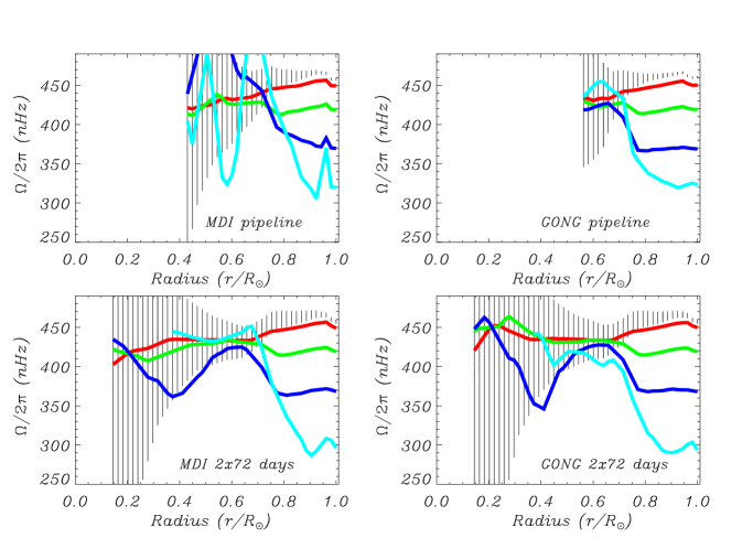
Figure 12.: Time-averaged rotational profiles obtained from the inversions of MDI $2\times 72$, GONG $2\times 72$-day long, GONG pipeline, and MDI pipeline. Black, red, green, dark-blue, and light-blue lines correspond to the rotational rate at different latitudes, namely $0,20,40,60$, and $80^{\rm o}$, respectively. Vertical lines represent the error bars for the rotational rate at the Equator.fig:29

5 Conclusions

We have fitted one solar cycle of MDI and GONG data and the latest HMI data using a new fitting methodology. This method fits individual multiplets, an asymmetric mode profile, incorporates all known instrumental distortion, uses our best estimate of the leakage matrix, and uses an optimal sine multi-tapered spectral estimator. It was applied to time series of varying lengths to study the effect of trading off precision for temporal resolution in the inversion results. On the other hand, the improved inversion method that we used is one that estimates the optimal inversion model grid based on the extent of the mode set (over spherical harmonic degree and frequency) and the data uncertainties.

Our results are summarized in Figure fig:18, where we present the rotational profiles obtained from inverting frequency splitting derived from fitting time series spanning an entire solar cycle, Cycle 23, for both GONG and MDI observations. These profiles are our best inferences of the rotation in the radiative region, to date. Both results are compatible with a radiative zone rotating rigidly at a rate of approximately 431 nHz; however, it is not possible to disregard a faster or slower rotator below $0.2{R_{\odot}}$ (i.e.  up to 600 or down to 300 nHz). Although the radiative zone seems to rotate rigidly, there is a consistent and systematic dip in the rotation profile located at around $0.4{R_{\odot}}$ and $60^{\rm o}$ of latitude. This dip appears to evolve with time, although this last result has to be confirmed when additional time series covering Cycle 24 become available.

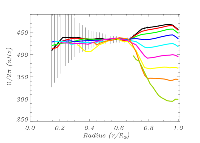
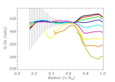
Figure 13.: Rotational profiles obtained from the inversions of MDI $64\times 72$ (left panel) and GONG $64\times 72$-day long (right panel). The rotational rates at different latitudes, from the Equator to $80^{\rm o}$ at steps of $10^{\rm o}$, are represented by colored lines. Vertical lines represent the error bars for the rotational rate at the Equator.fig:18

References

- Anderson, et al. (1990) Anderson, E.R., Duvall, T.L.Jr., Jefferies, S.M.: 1990, ApJ 364, 699, ADS: 1990ApJ…364..699A.
- Broomhall, et al. (2009) Broomhall, A.M., Chaplin, W.J., Davies, G.R., Elsworth, Y., Fletcher, S.T., Hale, S.J., Miller, B., New, R.: 2009, MNRAS 396, L100, ADS: 2009MNRAS.396L.100B, DOI: 10.1111/j.1745-3933.2009.00672.x.
- Duez, et al. (2010) Duez, V., Mathis, S., Turck-Chièze, S.: 2010, MNRAS 402, 271, ADS: 2010MNRAS.402..271D, DOI: 10.1111/j.1365-2966.2009.15955.x.
- Eff-Darwich, andPérez-Hernández (1997) Eff-Darwich, A., Pérez-Hernández, F.: 1997, A&AS 125, 1, ADS: 1997A&AS..125..391E, DOI: 10.1051/aas:1997229.
- Eff-Darwich, et al. (2002) Eff-Darwich, A., Korzennik, S.G., Jiménez-Reyes, S.J.: 2002, ApJ 573, 857, ADS: 2002ApJ…573..857E, DOI: 10.1086/340747.
- Eff-Darwich, et al. (2008) Eff-Darwich, A., Korzennik, S.G., Jiménez-Reyes, S.J., García, R.A.: 2008, ApJ 679, 1636, ADS: 2008ApJ…679.1636E, DOI: 10.1086/586724.
- Forgács-Dajka, andPetrovay (2001) Forgács-Dajka, E., Petrovay, K.: 2001, Sol. Phys. 203, 195, ADS: 2001SoPh..203..195F, DOI: 10.1023/A:1013389631585.
- Gabriel, et al. (1995) Gabriel, A.H., Grec, G., Charra, J.,Robillot, J.M., Roca Cortes, T., Turck-Chièze, S., Bocchia R., Boumier, P., Cantin, M., Cespédes, E., et al.: 1995, Sol. Phys. 162, 61, ADS: 1995SoPh..162…61G.
- García, et al. (2007) García, R.A.,Turck-Chièze, S., Jiménez-Reyes, S.J., Ballot, J., Pallé, P.L., Eff-Darwich, A., Mathur, S., Provost, J.: 2007, Science 316, 1591, ADS: 2007Sci…316.1591G, DOI: 10.1126/science.1140598.
- García, et al. (2008) García, R.A., Mathur, S., Ballot, J., et al.: 2008, Sol. Phys. 251, 119, ADS: 2008SoPh..251..119G, DOI: 10.1007/s11207-008-9144-5.
- Gough, andMcIntyre (1998) Gough, D.O., McIntyre, M.E.: 1998, Nature 394, 755, ADS: 1998Natur.394..755G, DOI: 10.1038/29472.
- Harvey, et al. (1996) Harvey, J.W., Hill, F., Hubbard, R.P., Kennedy, J.R., Leibacher, J.W., Pintar, J.A., et al.: 1996, Science 272, 1284, ADS: 1996Sci…272.1284H.
- Howe (2009) Howe, R.: 2009, Liv Rev in Solar Phys, http://solarphysics.livingreviews.org/Articles/lrsp-2009-1/ 6, 1.
- Korzennik (2005) Korzennik, S.G.: 2005, ApJ 626, 585, ADS: 2005ApJ…626..585K, DOI: 10.1086/429748.
- Korzennik (2008) Korzennik, S.G.: 2008, Phys. CS 118, 012082, ADS: 2008JPhCS.118a2082K, DOI: 10.1088/1742-6596/118/1/012082.
- Larson, and Schou (2008) Larson, T.P., Schou, J.: 2008, Phys. CS 118, 012083, ADS: 2008JPhCS.118a2083L, DOI: 10.1088/1742-6596/118/1/012083.
- Pijpers, andThompson (1994) Pijpers, F.P., Thompson, M.J.: 1994, A&A 281, 231, ADS: 1994A&A…281..231P.
- Salabert, et al. (2007) Salabert, D., Chaplin, W.J., Elsworth, Y., New, R., Verner, G.A.: 2007, A&A 463, 1181, ADS: 2007A&A…463.1181S, DOI: 10.1051/0004-6361:20066419.
- Scherrer, et al. (2012) Scherrer, P.H., Schou, J., Bush, R.I., Kosovichev, A.G., Bogart, R.S., Hoeksema, J.T., Liu, Y., Duvall, T.L., Zhao, J., Title, A.M., Schrijver, C.J., Tarbell, T.D., Tomczyk, S., 2012, Sol. Phys. 365, 207, ADS: 2012SoPh..275..207S, DOI: 10.1007/s11207-011-9834-2.
- Scherrer, et al. (1995) Scherrer, P.H.; Bogart, R.S.; Bush, R.I.; Hoeksema, J.T.; Kosovichev, A.G.; Schou et al.: 1995, Sol. Phys. 162, 129, ADS: 1995SoPh..162..129S, DOI: 10.1007/BF00733429.
- Schou (1992) Schou, J.: 1992, On the Analysis of Helioseismic Data, Ph.D. Thesis, Aarhus University, ADS: 1992PhDT…….380S.
- Starostenko, andZavorotko (1996) Starostenko, V.I., Zavorotko, A.N.: 1996, Comp. Geosci 22, 3, ADS: 1996CG…..22….3S, DOI: 10.1016/0098-3004(95)00052-6.
- Thompson, et al. (2003) Thompson, M.J., Christensen-Dalsgaard, J., Miesch, M.S., Toomre, J.: 2003, Ann. Rev. Astron. Astrophys. 41, 599, ADS: 2003ARA&A..41..599T, DOI: 10.1146/annurev.astro.41.011802.094848.
- Turck-Chièze, et al. (2010) Turck-Chièze, S., Palacios, A., Marques, J.P., Nghiem, P.A.P.: 2010, ApJ 715, 1539, ADS: 2010ApJ…715.1539T. DOI: 10.1146/annurev.astro.41.011802.094848.
- Woodard (1989) Woodard, M.F.: 1989, ApJ 347, 1176, ADS: 1989ApJ…347.1176W.
- Zahn, et al. (2007) Zahn, J.P., Brun, A.S., Mathis, S.: 2007, A&A 474, 145. ADS: 2007A&A…474..145Z, DOI: 10.1051/0004-6361:20077653.