Treatment of Calibration Uncertainty in Multi-Baseline Cross-Correlation Searches for Gravitational Waves

Abstract

Uncertainty in the calibration of gravitational-wave (GW) detector data leads to systematic errors which must be accounted for in setting limits on the strength of GW signals. When cross-correlation measurements are made using data from a pair of instruments, as in searches for a stochastic GW background, the calibration uncertainties of the individual instruments can be combined into an uncertainty associated with the pair. With the advent of multi-baseline GW observation (e.g., networks consisting of multiple detectors such as the LIGO observatories and Virgo), a more sophisticated treatment is called for. We describe how the correlations between calibration factors associated with different pairs can be taken into account by marginalizing over the uncertainty associated with each instrument.

1 Calibration Uncertainty with One Baseline

Consider an experiment to measure a physical quantity ${\mu}$ (e.g., the stochastic GW background strength $\Omega_{\mathrm{gw}}(f)$ [1, 2]). An optimal combination ${x}$ of cross-correlation measurements provides a point estimate of ${\mu}$ with error bar ${\sigma}$. Given a likelihood function $p({x}|{\mu})$ and a prior $p(\mu)$, one can use Bayes’s Theorem to construct the posterior

$$p({\mu}|{x})=\frac{p({x}|{\mu})p({\mu})}{p({x})}=\frac{p({x}|{\mu})p({\mu})}{\int d{\mu}\,p({x}|{\mu})\,p({\mu})}\,.$$ (1)

Due to calibration uncertainties in each of the instruments that make up the baseline for the cross-correlation, ${x}$ is an estimator not of ${\mu}$, but of ${\lambda}{\mu}$, where ${\lambda}$ is an unknown calibration factor (for the baseline) described by an uncertainty ${\varepsilon}$. Thus the likelihood function also depends on the calibration factor ${\lambda}$

$$p({x}|{\mu},{\lambda})=\frac{1}{{\sigma}\sqrt{2\pi}}\,\exp\left[-\frac{({x}-{\lambda}{\mu})^{2}}{2{\sigma}^{2}}\right]\ ,$$ (2)

so the posterior (1) is now constructed from the marginalized likelihood

$$p({x}|{\mu})=\int d{\lambda}\,p({x}|{\mu},{\lambda})p({\lambda})\ .$$ (3)

If we assume a Gaussian distribution for $\lambda$,

$$p({\lambda})=\frac{1}{{\varepsilon}\sqrt{2\pi}}\,\exp\left[-\frac{({\lambda}-1)^{2}}{2{\varepsilon}^{2}}\right]\ ,$$ (4)

then we can do the marginalization analytically if the range of $\lambda$ values is taken to be $(-\infty,\infty)$. This leads to

$$p({x}|{\mu})=\frac{1}{\sqrt{2\pi(\sigma^{2}+{\varepsilon}^{2}{\mu}^{2})}}\ \exp\left[-\frac{1}{2}\frac{(x-{\mu})^{2}}{(\sigma^{2}+{\varepsilon}^{2}{\mu}^{2})}\right]\,.$$ (5)

This is the method used in stochastic GW searches with two LIGO sites, e.g., [3, 4].

A more physically-motivated prior, which explicitly takes into account that $\lambda$ is multiplicative and takes on only positive values, is a log-normal distribution

$$p({\lambda})=\frac{1}{{\lambda}{\varepsilon}\sqrt{2\pi}}\,\exp\left[-\frac{(\ln{\lambda})^{2}}{2{\varepsilon}^{2}}\right]\quad{\rm or}\quad p({\Lambda})=\frac{1}{{\varepsilon}\sqrt{2\pi}}\,\exp\left[-\frac{{\Lambda}^{2}}{2{\varepsilon}^{2}}\right]\quad\hbox{where\ }{\Lambda}=\ln{\lambda}\,.$$ (6)

This was the approach taken in the stochastic GW search using LIGO and ALLEGRO [5], but has the drawback of requiring numerical integration over ${\Lambda}$ because

$$p({x}|{\mu},{\Lambda})=\frac{1}{{\sigma}\sqrt{2\pi}}\,\exp\left[-\frac{({x}-e^{{\Lambda}}{\mu})^{2}}{2{\sigma}^{2}}\right]$$ (7)

gives a factor which is not Gaussian in ${\Lambda}$. Figure 1 compares the posterior distributions for the two different choices of priors for different measured values of $x$ and different values of $\varepsilon$.

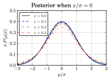
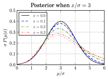
Figure 1: Effects of marginalizing analytically over a single calibration factor for two different values of the measured cross-correlation, $x=0$ and $x=3\sigma$. The thick line is a numerical marginalization with a log-normal prior on ${\lambda}$; the thin line is an analytic marginalization with a Gaussian prior on $\lambda$.

2 Calibration Uncertainty with Multiple Baselines

With more than two instruments, there are multiple baselines and multiple calibration uncertainties to marginalize over. For instance, the stochastic background search using initial LIGO and Virgo data [6, 7] involved 4 different instruments $I\in\{\mathrm{H1},\mathrm{H2},\mathrm{L1},\mathrm{V1}\}$ and 5 different baselines $\alpha\in\{\mathrm{H1L1},\mathrm{H1V1},\mathrm{H2L1},\mathrm{H2V1},\mathrm{L1V1}\}$.

Since the cross-correlation measurements for different baselines involve different calibration factors, all of the baselines cannot be optimally combined before marginalizing over calibration. Instead, all of the measurements for a baseline $\alpha$ can be combined into a single point estimate ${x_{\alpha}}$ with error bar ${\sigma_{\alpha}}$. Each baseline has unknown calibration factor ${\lambda_{\alpha}}$. Since the statistical errors for the different baselines are independent [8], the likelihood is the product

$$p(\mathbf{x}|{\mu},\boldsymbol{\lambda})=\prod_{\alpha}\left\{\frac{1}{{\sigma_{\alpha}}\sqrt{2\pi}}\,\exp\left[-\frac{({x_{\alpha}}-{\lambda_{\alpha}}{\mu})^{2}}{2{\sigma_{\alpha}}^{2}}\right]\right\}\ ,$$ (8)

where $\mathbf{x}\equiv\{x_{\alpha}\}$ and $\boldsymbol{\lambda}\equiv\{\lambda_{\alpha}\}$. The calibration factor ${\lambda_{\alpha}}$ for each baseline is ${\lambda_{IJ}}={\xi_{I}}{\xi_{J}}$, and is determined by the per-instrument calibration factors $\boldsymbol{\xi}\equiv\{\xi_{I}\}$. If each instrument’s calibration has an underlying uncertainty ${\delta_{I}}$, the per-baseline calibration factors $\boldsymbol{\lambda}$ have the following means, variances and covariances:

$$\left\langle{\lambda_{IJ}}\right\rangle=1\,,\quad\left\langle{\lambda_{IJ}\lambda_{IJ}}\right\rangle=1+{\delta_{I}}^{2}+{\delta_{J}}^{2}+\mathcal{O}({\delta}^{4});\quad\left\langle{\lambda_{IJ}\lambda_{JK}}\right\rangle=1+{\delta_{J}}^{2}+\mathcal{O}({\delta}^{4})\quad\hbox{if $I\neq K$}\ .$$ (9)

2.1 Per-Baseline Calibration Marginalization

One approach is to marginalize over the per-baseline calibration factors assuming a multivariate Gaussian prior $p(\boldsymbol{\lambda})$. This has the advantage that the marginalization integral

$$p(\mathbf{x}|{\mu})=\int d{\boldsymbol{\lambda}}\>p(\mathbf{x}|{\mu},\boldsymbol{\lambda})\,p(\boldsymbol{\lambda})$$ (10)

can be done analytically if the integrals over the per-baseline calibration factors $\boldsymbol{\lambda}$ are taken over $(-\infty,\infty)$. However, the relationship ${\lambda_{IJ}}={\xi_{I}}{\xi_{J}}$ implies that

$${\lambda_{IJ}}{\lambda_{KL}}-{\lambda_{IK}}{\lambda_{JL}}=0\ .$$ (11)

For a multivariate Gaussian prior on $\boldsymbol{\lambda}$, this relation is true only as an expectation value, not as an identity for all values of $\lambda_{IJ}$, $\lambda_{KL}$, etc.

2.2 Per-Instrument Calibration Marginalization

An alternative approach which enforces identities such as (11) is to set a prior which is the product of independent priors on each per-instrument calibration factor ${\xi_{I}}$ or equivalently on ${\Xi_{I}}=\ln{\xi_{I}}$. Similarly defining the log-calibration factor for a baseline ${\Lambda_{\alpha}}=\ln{\lambda_{\alpha}}$, we have

$${\Lambda_{IJ}}=\ln{\lambda_{IJ}}=\ln({\xi_{I}}{\xi_{J}})={\Xi_{I}}+{\Xi_{J}}\ .$$ (12)

The likelihood is

$$p(\mathbf{x}|{\mu},\boldsymbol{\Xi})=\prod_{\alpha}\left\{\frac{1}{{\sigma_{\alpha}}\sqrt{2\pi}}\,\exp\left[-\frac{({x_{\alpha}}-e^{{\Lambda_{\alpha}}}{\mu})^{2}}{2{\sigma_{\alpha}}^{2}}\right]\right\}$$ (13)

and the marginalized likelihood is

$$p(\mathbf{x}|{\mu})=\int d\boldsymbol{{\Xi}}\>p(\mathbf{x}|{\mu},\boldsymbol{\Xi})\,p(\boldsymbol{\Xi})\ .$$ (14)

An obvious prior is log-normal on $\xi_{I}$, i.e., Gaussian on $\Xi_{I}$:

$$p(\boldsymbol{\Xi})=\prod_{I}\left\{\frac{1}{{\delta_{I}}\sqrt{2\pi}}\,\exp\left(\frac{{\Xi_{I}}^{2}}{2{\delta_{I}}^{2}}\right)\right\}\ .$$ (15)

The exact integral over $\boldsymbol{\Xi}$ would need to be done numerically for each ${\mu}$, but if $\boldsymbol{\delta}$ are small, one can make the approximation $e^{{\Lambda_{IJ}}}\approx 1+{\Lambda_{IJ}}=1+{\Xi_{I}}+{\Xi_{J}}$ to convert the likelihood to a Gaussian integral over $\boldsymbol{\Xi}$ which can be done analytically. The result is a likelihood of the form

$$p(\mathbf{x}|{\mu})=\sqrt{\det\left(\frac{\mathbf{M}\bigl{(}{\mu},\boldsymbol{\sigma},\boldsymbol{\delta}\bigr{)}}{2\pi}\right)}\exp\left[-\frac{1}{2}\sum_{\alpha}\sum_{\beta}({x_{\alpha}}-{\mu})\,M_{\alpha\beta}\bigl{(}{\mu},\boldsymbol{\sigma},\boldsymbol{\delta}\bigr{)}\,({x_{\beta}}-{\mu})\right]\ .$$ (16)

This is the approach which was used for the multi-baseline upper limits in [7].

For the special case of two instruments which make up a single baseline, the matrix $\mathbf{M}$ reduces to a single number with value

$$\mathbf{M}\bigl{(}{\mu},\boldsymbol{\sigma},\boldsymbol{\delta}\bigr{)}\equiv\frac{1}{{\sigma_{12}^{2}}+{\mu}^{2}({\delta_{1}}^{2}+{\delta_{2}}^{2})}\,.$$ (17)

Comparing (17) to (5), we see that this approximation gives the same result as assuming a Gaussian prior in $\lambda_{12}$ with ${\varepsilon_{12}}^{2}={\delta_{1}}^{2}+{\delta_{2}}^{2}$.

3 Ongoing Work

More generally, we may be using $\mathbf{x}$ to estimate multiple physical quantities, such as different spherical harmonic modes of a non-isotropic stochastic GW background [9, 10]. These methods of analytic marginalization with either a multivariate Gaussian prior or an approximate likelihood function can be applied to the effects of calibration uncertainty in that search as well. Additionally, these calibration effects may also be considered in other cross-correlation searches, such as the modelled cross-correlation search for periodic GW signals.[11]

We wish to thank the organizers of the International Conference on Gravitation and Cosmology (ICGC 2011, Goa) and our colleagues in the LIGO Scientific Collaboration and the Virgo Collaboration, especially Albert Lazzarini. JTW was supported by NSF grant PHY-0855494. ELR was supported by the Max Planck Society. JDR was supported by NSF grants PHY-0855371 and HRD-0734800. EHT was supported by NSF grant PHY-0758035. This paper has been assigned LIGO Document Number P1200051-v4.

References

References

[1]
Christensen N L 1992 Phys. Rev.D46, 5250
[2]
Allen B and Romano JD 1999 Phys. Rev.D59, 102001
[3] Abbott B et al (LIGO Scientific Collaboration)
2007 Astrophys. J659, 918
[4] Abbott B P et al (LIGO Scientific Collaboration and
Virgo) 2009 Nature460, 990
[5] Abbott B et al (LIGO Scientific Collaboration and
ALLEGRO) 2007 Phys. Rev.D76, 022001
[6] Cella G et al 2007 Class. Quant. Grav.24, S639
[7] Abadie J et al (LIGO Scientific Collaboration and
Virgo) 2012 Phys. Rev.D85, 122001
[8] Lazzarini A et al 2004 Phys. Rev.D70, 062001
[9] Thrane E et al 2009 Phys. Rev.D80, 122002
[10] Abadie J et al (LIGO Scientific Collaboration and
Virgo) 2011 Phys. Rev. Lett.107, 271102
[11] Dhurandhar S et al 2008 Phys. Rev.D77, 082001