Efficient Assembly of $H(\mathrm{div})$ and $H(\mathrm{curl})$ Conforming Finite Elements

Abstract

In this paper, we discuss how to efficiently evaluate and assemble general finite element variational forms on $H(\mathrm{div})$ and $H(\mathrm{curl})$. The proposed strategy relies on a decomposition of the element tensor into a precomputable reference tensor and a mesh-dependent geometry tensor. Two key points must then be considered: the appropriate mapping of basis functions from a reference element, and the orientation of geometrical entities. To address these issues, we extend here a previously presented representation theorem for affinely mapped elements to Piola-mapped elements. We also discuss a simple numbering strategy that removes the need to contend with directions of facet normals and tangents. The result is an automated, efficient, and easy-to-use implementation that allows a user to specify finite element variational forms on $H(\mathrm{div})$ and $H(\mathrm{curl})$ in close to mathematical notation.

10.1137/08073901X

1 Introduction

The Sobolev spaces $H(\mathrm{div})$ and $H(\mathrm{curl})$ play an important role in many applications of mixed finite element methods to partial differential equations. Examples include second order elliptic partial differential equations, Maxwell’s equations for electromagnetism, and the linear elasticity equations. Mixed finite element methods may provide advantages over standard $H^{1}$ finite element discretizations in terms of added robustness, stability, and flexibility. However, implementing $H(\mathrm{div})$ and $H(\mathrm{curl})$ methods requires additional code complexity for constructing basis functions and evaluating variational forms, which helps to explain their relative scarcity in practice.

The FEniCS project [15, 26] comprises a collection of free software components for the automated solution of differential equations. One of these components is the FEniCS form compiler (FFC) [20, 21, 25]. FFC allows finite element spaces over simplicial meshes and multilinear forms to be specified in a form language close to the mathematical abstraction and notation. The form compiler generates low-level (C++) code for efficient form evaluation and assembly based on an efficient tensor contraction. Moreover, the FErari project [19, 22, 23, 24] has developed specialized techniques for further optimizing this code based on underlying discrete structure. FFC relies on the FInite element Automatic Tabulator (FIAT) [16, 17, 18] for the tabulation of finite element basis functions. FIAT provides methods for efficient tabulation of finiteelement basis functions and their derivatives at any particular point. In particular, FIAT provides simplicial $H(\mathrm{div})$ element spaces such as the families of Raviart and Thomas [34], Brezzi, Douglas, and Marini [10], and Brezzi et al. [9], as well as $H(\mathrm{curl})$ elements of the Nédélec types [29, 30].

Previous iterations of FFC have enabled easy use of $H^{1}$ and $L^{2}$ conforming finite element spaces, including discontinuous Galerkin formulations, but support for $H(\mathrm{div})$ and $H(\mathrm{curl})$ spaces has been absent. In this paper, we extend the previous work [20, 21, 31] to allow simple and efficient compilation of variational forms on $H(\mathrm{div})$ and $H(\mathrm{curl})$, including mixed formulations on combinations of $H^{1}$, $H(\mathrm{div})$, $H(\mathrm{curl})$, and $L^{2}$. The efficiency of the proposed approach relies, in part, on the tensor representation framework established in [21]. In this framework, the element tensor is represented as the contraction of a reference tensor and a geometry tensor. The former can be efficiently precomputed given automated tabulation of finite element basis functions on a reference element, while the latter depends on the geometry of each physical element. For this strategy, a key aspect of the assembly of $H(\mathrm{div})$ and $H(\mathrm{curl})$ conforming element spaces becomes the Piola transformations, isomorphically mapping basis functions from a reference element to each physical element. Also, the orientation of geometrical entities such as facet tangents and normals must be carefully considered.

Implementations of $H(\mathrm{div})$ and $H(\mathrm{curl})$ finite element spaces, in particular of arbitrary degree, are not prevalent. There are, to our knowledge, no implementations that utilize the compiled approach to combine the efficiency of low-level optimized code with a fully automated high-level interface. Some finite element packages, such as FEAP [1], do not provide $H(\mathrm{div})$ or $H(\mathrm{curl})$ type elements at all. Others, such as FreeFEM [33], typically provide only low-order elements such as the lowest-order Raviart–Thomas elements. Some libraries such as deal.II [8] or FEMSTER [12] do provide arbitrary degree elements of Raviart–Thomas and Nédélec type, but do not automate the evaluation of variational forms. NGSolve [36] provides arbitrary order $H(\mathrm{div})$ and $H(\mathrm{curl})$ elements along with automated assembly, but only for a predefined set of bilinear forms.

This exposition and the FFC implementation consider the assembly of $H(\mathrm{div})$ and $H(\mathrm{curl})$ finite element spaces on simplicial meshes. However, the underlying strategy is extendible to nonsimplicial meshes and tensor-product finite element spaces defined on such meshes. A starting point for an extension to isoparametric $H^{1}$ conforming finite elements was discussed in [20]. The further extensions to $H(\mathrm{div})$ and $H(\mathrm{curl})$ follow the same lines as for the simplicial case discussed in this note.

The outline of this paper is as follows. We begin by reviewing basic aspects of the function spaces $H(\mathrm{div})$ and $H(\mathrm{curl})$ in section 2, and we provide examples of variational forms defined on these spaces. We continue, in section 3, by summarizing the $H(\mathrm{div})$ and $H(\mathrm{curl})$ conforming finite elements implemented by FIAT. In section 4, we recap the multilinear form framework of FFC and we present an extension of the representation theorem from [21]. Subsequently, in section 5, we provide some notes on the assembly of $H(\mathrm{div})$ and $H(\mathrm{curl})$ elements. Particular emphasis is placed on aspects not easily found in the standard literature, such as the choice of orientation of geometric entities. In section 6, we return to the examples introduced in section 2 and illustrate the ease and terseness with which even complicated mixed finite element formulations may be expressed in the FFC form language. Convergence rates in agreement with theoretically predicted results are presented to substantiate the veracity of the implementation. Finally, we make some concluding remarks in section 7.

2 $H(\mathrm{div})$ and $H(\mathrm{curl})$

In this section, we summarize some basic facts about the Sobolev spaces $H(\mathrm{div})$ and $H(\mathrm{curl})$ and we discuss conforming finite element spaces associated with them. Our primary focus is on properties relating to interelement continuity and change of variables. The reader is referred to the monographs [11] and [28] for a more thorough analysis of $H(\mathrm{div})$ and $H(\mathrm{curl})$, respectively.

2.1 Definitions

For an open domain $\Omega\subset\mathbb{R}^{n}$, we let $L^{2}(\Omega,\mathbb{R}^{n})$ denote the space of square-integrable vector fields on $\Omega$ with the associated norm $||\cdot||_{0}$ and inner-product $\langle\cdot,\cdot\rangle$, and we abbreviate $L^{2}(\Omega)=L^{2}(\Omega,\mathbb{R}^{1})$. We define the following standard differential operators on smooth fields $v$: $D^{\alpha}v=\partial_{x_{1}}^{\alpha_{1}}\cdots\partial_{x_{m}}^{\alpha_{m}}v$ for a multi-index $\alpha$ of length $m$, $\operatorname{div}v=\sum_{i=1}^{n}\partial_{x_{i}}v_{i}$, $\operatorname{curl}v=(\partial_{x_{2}}v_{3}-\partial_{x_{3}}v_{2},\partial_{x_{3}}v_{1}-\partial_{x_{1}}v_{3},\partial_{x_{1}}v_{2}-\partial_{x_{2}}v_{1})$, and $\operatorname{rot}v=\partial_{x_{1}}v_{2}-\partial_{x_{2}}v_{1}$. We may then define the spaces $H^{m}(\Omega)$, $H(\mathrm{div};\Omega)$, and $H(\mathrm{curl};\Omega)$ by

$$H^{m}(\Omega) =\{v\in L^{2}(\Omega):\;D^{\alpha}v\in L^{2}(\Omega),\;|\alpha|\leq m\},\quad m=1,2,\dots,$$

$$H(\mathrm{div};\Omega) =\{v\in L^{2}(\Omega,\mathbb{R}^{n}):\;\operatorname{div}v\in L^{2}(\Omega)\},$$

$$H(\mathrm{curl};\Omega) =\left\{\begin{tabular}[]{ll}$\{v\in L^{2}(\Omega,\mathbb{R}^{2}):\;\operatorname{rot}v\in L^{2}(\Omega)\}$,&$\Omega\subset\mathbb{R}^{2}$,\\ $\{v\in L^{2}(\Omega,\mathbb{R}^{3}):\;\operatorname{curl}v\in L^{2}(\Omega,\mathbb{R}^{3})\}$,&$\Omega\subset\mathbb{R}^{3}$,\end{tabular}\right.$$

with derivatives taken in the distributional sense. The reference to the domain $\Omega$ will be omitted when appropriate, and the associated norms will be denoted $||\cdot||_{m}$, $||\cdot||_{\operatorname{div}}$, and $||\cdot||_{\operatorname{curl}}$. Furthermore, we let $\mathbb{M}$ denote the space of matrices and we let $H(\operatorname{div};\Omega,\mathbb{M})$ denote the space of square-integrable matrix fields with square-integrable row-wise divergence.

For the sake of compact notation, we shall also adopt the exterior calculus notation of [5] and let $\Lambda^{k}(\Omega)$ denote the space of smooth differential $k$-forms on $\Omega$, and let $L^{2}\Lambda^{k}(\Omega)$ denote the space of square-integrable differential $k$-forms on $\Omega$. We further let $\operatorname{d}$ denote the exterior derivative with adjoint $\operatorname{\delta}$, and we define $H\Lambda^{k}(\Omega)=\{v\in L^{2}\Lambda^{k}(\Omega),\operatorname{d}v\in L^{2}\Lambda^{k}(\Omega)\}$. Further, $\mathcal{P}_{r}\Lambda^{k}$ is the space of polynomial $k$-forms of up to and including degree $r$, and $\mathcal{P}^{-}_{r}\Lambda^{k}$ denotes the reduced space as defined in [5, section 3.3].

2.2 Examples

The function spaces $H(\mathrm{div})$ and $H(\mathrm{curl})$ are the natural function spaces for an extensive range of partial differential equations, in particular in mixed formulations. We sketch some examples in the following, both for motivational purposes and for later reference. The examples considered here are mixed formulations of the Hodge Laplace equations, the standard eigenvalue problem for Maxwell’s equations, and a mixed formulation for linear elasticity with weakly imposed symmetry. We return to these examples in section 6.

Example 2.1 (mixed formulation of Poisson’s equation).

The most immediate example involving the space $H(\mathrm{div})$ is a mixed formulation of Poisson’s equation: $-\Delta u=f$ in $\Omega\subset\mathbb{R}^{n}$. By introducing the flux $\sigma=-\operatorname{grad}u$ and assuming Dirichlet boundary conditions for $u$, we obtain the following mixed variational problem: Find $\sigma\in H(\mathrm{div};\Omega)$ and $u\in L^{2}(\Omega)$ satisfying

(1) $$\langle\tau,\sigma\rangle-\langle\operatorname{div}\tau,u\rangle+\langle v,\operatorname{div}\sigma\rangle=\langle v,f\rangle$$

for all $\tau\in H(\mathrm{div};\Omega)$ and $v\in L^{2}(\Omega)$.

Example 2.2 (the Hodge Laplacian).

With more generality, we may consider weak formulations of the Hodge Laplacian equation $(\operatorname{d}\operatorname{\delta}+\operatorname{\delta}\operatorname{d})u=f$ on a domain $\Omega\subset\mathbb{R}^{n}$; see [5, section 7]. For simplicity of presentation, we assume that $\Omega$ is contractible such that the space of harmonic forms on $\Omega$ vanishes. The formulation in Example 2.1 is the equivalent of seeking $u\in H\Lambda^{n}$ and $\sigma=\operatorname{\delta}u\in H\Lambda^{n-1}$ for $n=2,3$ with natural boundary conditions (the appropriate trace being zero). To see this, we test $\sigma=\operatorname{\delta}u$ against $\tau\in H\Lambda^{n-1}$ and we test $(\operatorname{d}\operatorname{\delta}+\operatorname{\delta}\operatorname{d})u=f$ against $v\in H\Lambda^{n}$ to obtain

$$\langle\tau,\sigma\rangle-\langle\tau,\operatorname{\delta}u\rangle+\langle v,\operatorname{d}\sigma\rangle=\langle v,f\rangle,$$

noting that $du=0$ for $u\in H\Lambda^{n}$. Integrating by parts, we obtain

(2) $$\langle\tau,\sigma\rangle-\langle\operatorname{d}\tau,u\rangle+\langle v,\operatorname{d}\sigma\rangle=\langle v,f\rangle.$$

We may restate (2) in the form (1) by making the identifications $\operatorname{\delta}u=-\operatorname{grad}u$, $\operatorname{d}\tau=\operatorname{div}\tau$, and $\operatorname{d}\sigma=\operatorname{div}\sigma$. If $\Omega\subset\mathbb{R}^{3}$, we may also consider the following mixed formulations of the Hodge Laplace equation.

1. Find $\sigma\in H\Lambda^{1}=H(\mathrm{curl})$ and $u\in H\Lambda^{2}=H(\mathrm{div})$ such that

   (3) $$\langle\tau,\sigma\rangle-\langle\operatorname{curl}\tau,u\rangle+\langle v,\operatorname{curl}\sigma\rangle+\langle\operatorname{div}v,\operatorname{div}u\rangle=\langle v,f\rangle$$

   for all $\tau\in H\Lambda^{1}$, $v\in H\Lambda^{2}$.

2. Find $\sigma\in H\Lambda^{0}=H^{1}$ and $u\in H\Lambda^{1}=H(\mathrm{curl})$ such that

   (4) $$\langle\tau,\sigma\rangle-\langle\operatorname{grad}\tau,u\rangle+\langle v,\operatorname{grad}\sigma\rangle+\langle\operatorname{curl}v,\operatorname{curl}u\rangle=\langle v,f\rangle$$

   for all $\tau\in H\Lambda^{0},v\in H\Lambda^{1}$.

Example 2.3 (cavity resonator).

The time-harmonic Maxwell equations in a cavity with perfectly conducting boundary induces the following eigenvalue problem: Find resonances $\omega\in\mathbb{R}$ and eigenfunctions $E\in H_{0}(\operatorname{curl};\Omega)$, satisfying

(5) $$\langle\operatorname{curl}F,\operatorname{curl}E\rangle=\omega^{2}\langle F,E\rangle\quad\forall F\in H_{0}(\operatorname{curl};\Omega),$$

where $H_{0}(\operatorname{curl};\Omega)=\{v\in H(\mathrm{curl};\Omega)|\;v\times n|_{\partial\Omega}=0\}$. Note that the formulation (5) disregards the original divergence-free constraint for the electric field $E$ and thus includes the entire kernel of the $\operatorname{curl}$ operator, corresponding to $\omega=0$ and electric fields of the form $E=\operatorname{grad}\psi$.

Example 2.4 (elasticity with weakly imposed symmetry).

Navier’s equations for linear elasticity can be reformulated using the stress tensor $\sigma$, the displacement $u$, and an additional Lagrange multiplier $\gamma$ corresponding to the symmetry of the stress constraint. The weak equations for $\Omega\subset\mathbb{R}^{2}$, with the natural boundary condition $u|_{\partial\Omega}=0$, take the following form: Given $f\in L^{2}(\Omega,\mathbb{R}^{n})$, find $\sigma\in H(\operatorname{div};\Omega,\mathbb{M})$, $u\in L^{2}(\Omega,\mathbb{R}^{n})$, and $\gamma\in L^{2}(\Omega)$ such that

(6) $$\langle\tau,A\sigma\rangle+\langle\operatorname{div}\tau,u\rangle+\langle v,\operatorname{div}\sigma\rangle+\langle\operatorname{skw}\tau,\gamma\rangle+\langle\eta,\operatorname{skw}\sigma\rangle=\langle v,f\rangle$$

for all $\tau\in H(\operatorname{div};\Omega,\mathbb{M})$, $v\in L^{2}(\Omega,\mathbb{R}^{n})$, and $\eta\in L^{2}(\Omega)$. Here, $A$ is the compliance tensor, and $\operatorname{skw}\tau$ is the scalar representation of the skew-symmetric component of $\tau$; more precisely, $2\operatorname{skw}\tau=\tau_{21}-\tau_{12}$. This formulation has the advantage of being robust with regard to nearly incompressible materials and it provides an alternative foundation for complex materials with nonlocal stress-strain relations. For more details, we refer the reader to [6].

2.3 Continuity-preserving mappings for $H(\mathrm{div})$ and $H(\mathrm{curl})$

At this point, we turn our attention to a few results on continuity-preserving mappings for $H(\mathrm{div})$ and $H(\mathrm{curl})$. The results are classical and we refer the reader to [11, 28] for a more thorough treatment.

First, it follows from Stokes’ theorem that in order for piecewise $H(\mathrm{div})$ vector fields to be in $H(\mathrm{div})$ globally, the traces of the normal components over patch interfaces must be continuous, and analogously tangential continuity is required for piecewise $H(\mathrm{curl})$ fields. More precisely, we have the following: Let $\mathcal{T}_{h}=\{K\}$ be a partition of $\Omega$ into subdomains. Define the space $\Sigma_{h}$ of piecewise $H(\mathrm{div})$ functions relative to this partition $\mathcal{T}_{h}$:

(7) $$\Sigma_{h}=\{\phi\in L^{2}(\Omega,\mathbb{R}^{n}):\;\phi|_{K}\in H(\operatorname{div};K)\ \forall K\in\mathcal{T}_{h}\}.$$

Then $\phi\in\Sigma_{h}$ is in $H(\mathrm{div};\Omega)$ if and only if the normal traces of $\phi$ are continuous across all element interfaces. Analogously, if $\phi|_{K}\in H(\operatorname{curl};K)$ for all $K\in\mathcal{T}_{h}$, then $\phi\in H(\mathrm{curl};\Omega)$ if and only if the tangential traces are continuous across all element interfaces.

Second, we turn to consider a nondegenerate mapping $F:\Omega_{0}\rightarrow F(\Omega_{0})=\Omega$ with Jacobian $DF(X)$, $X\in\Omega_{0}\subset\mathbb{R}^{n}$. For $\Phi\in H^{m}(\Omega_{0})$, the mapping $\mathcal{F}$ defined by

(8) $$\mathcal{F}(\Phi)=\Phi\circ F^{-1}$$

is an isomorphism from $H^{m}(\Omega_{0})$ to $H^{m}(\Omega)$. This, however, is not the case for $H(\mathrm{div})$ or $H(\mathrm{curl})$, since $\mathcal{F}$ does not in general preserve continuity of normal or tangential traces. Instead, one must consider the contravariant and covariant Piola mappings which preserve normal and tangential continuity, respectively.

Definition 2.5 (the contravariant and covariant Piola mappings).

Let $\Omega_{0}\subset\mathbb{R}^{n}$, let $F$ be a nondegenerate mapping from $\Omega_{0}$ onto $F(\Omega_{0})=\Omega$ with $J=DF(X)$, and let $\Phi\in L^{2}(\Omega_{0},\mathbb{R}^{n})$.

The contravariant Piola mapping $\mathcal{F}^{\mathrm{div}}$ is defined by

(9) $$\mathcal{F}^{\mathrm{div}}(\Phi)=\frac{1}{\det J}J\Phi\circ F^{-1}.$$

The covariant Piola mapping $\mathcal{F}^{\mathrm{curl}}$ is defined by

(10) $$\mathcal{F}^{\mathrm{curl}}(\Phi)=J^{-T}\Phi\circ F^{-1}.$$

Remark 2.6.

We remark that the contravariant Piola mapping is usually defined with an absolute value, $\mathcal{F}^{\mathrm{div}}(\Phi)=\frac{1}{|\det J|}J\Phi\circ F^{-1}$. However, omitting the absolute value, as in (9), can simplify the assembly of $H(\mathrm{div})$ elements, as will be expounded in section 5.

The contravariant Piola mapping is an isomorphism of $H(\operatorname{div};\Omega_{0})$ onto $H(\mathrm{div};\Omega)$, and the covariant Piola mapping is an isomorphism of $H(\operatorname{curl};\Omega_{0})$ onto $H(\mathrm{curl};\Omega)$. In particular, the contravariant Piola mapping preserves normal traces, and the covariant Piola mapping preserves tangential traces. We illustrate this below in the case of simplicial meshes in two and three space dimensions (triangles and tetrahedra). The same results hold for nonsimplicial meshes with cell-varying Jacobians, such as quadrilateral meshes [4, 11].

Example 2.7 (Piola mapping on triangles in $\mathbb{R}^{2}$).

Let $K_{0}$ be a triangle with vertices $X^{i}$ and edges $E^{i}$ for $i=1,2,3$. We define the unit tangents by $T^{i}=E^{i}/||E^{i}||$. We further define the unit normals by $N^{i}=RT^{i}$, where

(11) $$R=\begin{pmatrix}0&1\\ -1&0\end{pmatrix}$$

is the clockwise rotation matrix.

Now, assume that $K_{0}$ is affinely mapped to a (nondegenerate) simplex $K$ with vertices $x^{i}$. The affine mapping $F_{K}:K_{0}\rightarrow K$ takes the form $x=F_{K}(X)=JX+b$ and satisfies $x^{i}=F_{K}(X^{i})$ for $i=1,2,3$. It follows that edges are mapped by

$$e=x^{i}-x^{j}=J(X^{i}-X^{j})=JE.$$

Similarly, normals are mapped by

$$||e||n=Re=RJE=(\det J)J^{-T}RE=(\det J)J^{-T}||E||N,$$

where we have used that $\frac{1}{\det J}RJR^{T}=J^{-T}$ and thus $RJ=(\det J)J^{-T}R$ for $J\in\mathbb{R}^{2\times 2}$.

The relation between the mappings of tangents and normals (or edges and rotated edges) may be summarized in the following commuting diagrams:

(12) $$\begin{CD}T@>{J||E||/||e||}>{}>t\\ @V{R}V{}V@V{}V{R}V\\ N@>{(\det J)J^{-T}||E||/||e||}>{}>n\end{CD}\quad\quad\quad\begin{CD}E@>{J}>{}>e\\ @V{R}V{}V@V{}V{R}V\\ ||E||N@>{(\det J)J^{-T}}>{}>||e||n\end{CD}$$

\psfrag{0}{$1$}\psfrag{1}{$2$}\psfrag{2}{$3$}\psfrag{K0}{$K_{0}$}\psfrag{K}{$K$}\psfrag{Fn}{$\Phi_{n}(X)=(\frac{1}{\sqrt{2}},\frac{1}{\sqrt{2}})$}\psfrag{Ft}{$\Phi_{t}(X)=(-\frac{1}{\sqrt{2}},\frac{1}{\sqrt{2}})$}\psfrag{fn1}{$\phi_{n}(x)=(1,\frac{1}{2})$}\psfrag{ft1}{$\phi_{t}(x)=(0,\frac{1}{2})$}\psfrag{fn2}{$\phi_{n}(x)=(\frac{1}{2},0)$}\psfrag{ft2}{$\phi_{t}(x)=(-\frac{1}{2},1)$}\psfrag{x}{$x$}\psfrag{X}{$X$}\psfrag{Fdiv}{$\mathcal{F}^{\mathrm{div}}$}\psfrag{Fcurl}{$\mathcal{F}^{\mathrm{curl}}$}\includegraphics[width=381.5877pt]{eps/piolaexample.eps}

Fig. 1: Mapping two vector fields $\Phi_{n}$ and $\Phi_{t}$ between two triangles using the contravariant and covariant Piola mappings. The contravariant Piola mapping (above) preserves normal traces of vector fields, and the covariant Piola mapping (below) preserves tangential traces of vector fields. This means in particular that the contravariant Piola mapping maps tangents to tangents (which have a zero normal component), and that the covariant Piola mapping maps normals to normals (which have a zero tangential component). Note that this is somewhat counterintuitive; the contravariant $H(\mathrm{div})$ Piola mapping always maps tangential fields to tangential fields but does not in general map normal fields to normal fields. However, in both cases the normal component (being zero and one, respectively) is preserved.

With this in mind, we may study the effect of the Piola transforms on normal and tangential traces. Let $\Phi\in C^{\infty}(K_{0},\mathbb{R}^{n})$ and let $\phi=\mathcal{F}^{\mathrm{div}}(\Phi)$. Then

$$||e||\,\phi(x)\cdot n=||e||\left((\det J)^{-1}J\Phi(X)\right)^{T}\left((\det J)J^{-T}||E||/||e||N\right)=||E||\,\Phi(X)\cdot N.$$

Thus, the contravariant Piola mapping preserves normal traces for vector fields under affine mappings, up to edge lengths. In general, the same result holds for smooth, nondegenerate mappings $F_{K}$ if the Jacobian $DF_{K}(X)$ is invertible for all $X\in K_{0}$.

Similarly, let $\phi=\mathcal{F}^{\mathrm{curl}}(\Phi)$. Then

(13) $$||e||\,\phi(x)\cdot t=||e||\left(J^{-T}\Phi(X)\right)^{T}\left(J||E||/||e||\right)=||E||\,\Phi(X)\cdot T.$$

Thus, the covariant Piola preserves tangential traces for vector fields, again up to edge lengths. Observe that the same result holds for tetrahedra without any modifications. The effect of the contravariant and covariant Piola mappings on normal and tangential traces is illustrated in Figure 1, where $||E||=||e||$ for simplicity.

Example 2.8 (contravariant Piola mapping on tetrahedra in $\mathbb{R}^{3}$).

Now, let $K_{0}$ be a tetrahedron. As explained above, the covariant Piola mapping preserves tangential traces. To study the effect of the contravariant Piola mapping on normal traces, we define the face normals of $K$ by $N=\frac{E^{i}\times E^{j}}{||E^{i}\times E^{j}||}$. Then

$$||e^{i}\times e^{j}||n=JE^{i}\times JE^{j}=\det JJ^{-T}(E^{i}\times E^{j})=||E^{i}\times E^{j}||\det JJ^{-T}N,$$

since $(Ju)\times(Jv)=\det JJ^{-T}(u\times v)$. Let $\Phi\in C^{\infty}(K_{0},\mathbb{R}^{n})$ and let $\phi=\mathcal{F}^{\mathrm{div}}(\Phi)$. Then, it follows that

$$||e^{i}\times e^{j}||\,\phi(x)\cdot n=||E^{i}\times E^{j}||\,\Phi(X)\cdot N.$$

Thus, the contravariant Piola mapping preserves normal traces, up to the area of faces.

We finally remark that if $J\in\mathbb{R}^{2\times 2}$ defines a conformal, orientation-preserving map, the contravariant and covariant Piola mappings coincide. In $\mathbb{R}^{3}$, $J$ must also be orthogonal for this to occur.

3 $H(\mathrm{div})$ and $H(\mathrm{curl})$ conforming finite elements

To construct $H(\mathrm{div})$ and $H(\mathrm{curl})$ conforming finite element spaces, that is, discrete spaces $V_{h}$ satisfying $V_{h}\subset H(\mathrm{div})$ or $V_{h}\subset H(\mathrm{curl})$, one may patch together local function spaces (finite elements) and make an appropriate matching of degrees of freedom over shared element facets. Here, a facet denominates any geometric entity of positive codimension in the mesh (such as an edge of a triangle or an edge or face of a tetrahedron). In particular, one requires that degrees of freedom corresponding to normal traces match for $H(\mathrm{div})$ conforming discretizations and that tangential traces match for $H(\mathrm{curl})$ conforming discretizations.

Several families of finite element spaces with degrees of freedom chosen to facilitate this exist. For $H(\mathrm{div})$ on simplicial tessellations in two dimensions, the classical conforming families are those of Raviart and Thomas ($\mathrm{RT}_{r}$, $r=0,1,2,\dots$) [34]; Brezzi, Douglas, and Marini ($\mathrm{BDM}_{r}$, $r=1,2,\dots$) [10]; and Brezzi et al. ($\mathrm{BDFM}_{r}$, $r=1,2,\dots$) [9]. The former two families were extended to three dimensions by Nédélec [29, 30]. However, the same notation will be used for the two- and three-dimensional $H(\mathrm{div})$ element spaces here. For $H(\mathrm{curl})$, there are the families of Nédélec of the first kind ($\mathrm{NED}_{r}^{1}$, $r=0,1,2,\dots$) [29] and of the second kind ($\mathrm{NED}_{r}^{2}$, $r=1,2,\dots$) [30]. We summarize in Table 1 those $H(\mathrm{div})$ and $H(\mathrm{curl})$ conforming finite elements that are supported by FIAT and hence by FFC. In general, FFC can wield any finite element space that may be generated from a local basis through either of the aforedescribed mappings. In Table 2, we also summarize some basic approximation properties of these elements for later comparison with numerical results in section 6.

Table 1: $H(\mathrm{div})$ and $H(\mathrm{curl})$ conforming finite elements on triangles and tetrahedra supported by FIAT and FFC for $r\geq 1$. When applicable, the elements are listed with their exterior calculus notation, along with their original references. Note that for $K\subset\mathbb{R}^{3}$, the Raviart–Thomas and Brezzi–Douglas–Marini elements are also known as the first and second kind $H(\mathrm{div})$ Nédélec (face)elements, respectively.

Simplex	$H(\mathrm{div})$	$H(\mathrm{curl})$
$K\subset\mathbb{R}^{2}$	$\mathrm{BDM}_{r}$ $\mathcal{P}_{r}\Lambda^{1}(K)$ [10] $\mathrm{RT}_{r-1}$ $\mathcal{P}_{r}^{-}\Lambda^{1}(K)$ [34] $\mathrm{BDFM}_{r}$ — [9]	$\mathrm{NED}^{1}_{r-1}$ —
$K\subset\mathbb{R}^{3}$	$\mathrm{BDM}_{r}$ $\mathcal{P}_{r}\Lambda^{2}(K)$ [30] $\mathrm{RT}_{r-1}$ $\mathcal{P}_{r}^{-}\Lambda^{2}(K)$ [29] $\mathrm{BDFM}_{r}$ —	$\mathrm{NED}^{1}_{r-1}$ $\mathcal{P}_{r}^{-}\Lambda^{1}(K)$ [29]

Table 2: Approximation properties of the spaces from Table 1. $C>0$, $r\geq 1$, $1\leq m\leq r$. $\Pi_{h}$ denotes the canonical interpolation operator, defined by the degrees of freedom, onto the element space in question. For simplicity, it is assumed that $v$ is sufficiently smooth for the interpolation operators to be well-defined, and for the given norms to be bounded. For more details and sharper estimates; cf. [11, 28].

Finite element	Interpolation estimates
$\mathcal{P}_{r}\Lambda^{k}(\Omega)$	$||v-\Pi_{h}v||_{0}\leq Ch^{m+1}||v||_{m+1}$,	$||v-\Pi_{h}v||_{\operatorname{div},\operatorname{curl}}\leq Ch^{m}||v||_{m+1}$
$\mathcal{P}_{r}^{-}\Lambda^{k}(\Omega)$	$||v-\Pi_{h}v||_{0}\leq Ch^{m}||v||_{m}$,	$||v-\Pi_{h}v||_{\operatorname{div},\operatorname{curl}}\leq Ch^{m}||v||_{m+1}$
$\mathrm{BDFM}_{r}$	$||v-\Pi_{h}v||_{0}\leq Ch^{m}||v||_{m}$,	$||v-\Pi_{h}v||_{\operatorname{div}}\leq Ch^{m}||v||_{m+1}$

For the reasons above, it is common to define the degrees of freedom for each of the elements in Table 1 as moments of either normal or tangential traces over element facets. However, one may alternatively consider point values of traces at suitable points on element facets (in addition to any internal degrees of freedom). Thus, the degrees of freedom for the lowest order Raviart–Thomas space on a triangle may be chosen as the normal components at the edge midpoints, and for the lowest order Brezzi–Douglas–Marini space, we may consider the normal components at two points on each edge (positioned symmetrically on each edge and not touching the vertices). This, along with the appropriate scaling by edge length, is how the degrees of freedom are implemented in FIAT.

4 Representation of $H(\mathrm{div})$ and $H(\mathrm{curl})$ variational forms

In this section, we discuss how multilinear forms on $H(\mathrm{div})$ or $H(\mathrm{curl})$ may be represented as a particular tensor contraction, allowing for precomputation of integrals on a reference element and thus efficient assembly of linear systems. We follow the notation from [20, 21] and extend the representation theorem from [21] for multilinear forms on $H^{1}$ and $L^{2}$ to $H(\mathrm{div})$ and $H(\mathrm{curl})$. The main new component is that we must use the appropriate Piola mapping to map basis functions from the reference element.

4.1 Multilinear forms and their representation

Let $\Omega\subset\mathbb{R}^{n}$ and let $\{V_{h}^{j}\}_{j=1}^{\rho}$ be a set of finite dimensional spaces associated with a tessellation $\mathcal{T}=\{K\}$ of $\Omega$. We consider the following canonical linear variational problem: Find $u_{h}\in V_{h}^{2}$ such that

(14) $$a(v,u_{h})=L(v)\quad\forall v\in V_{h}^{1},$$

where $a$ and $L$ are bilinear and linear forms on $V_{h}^{1}\times V_{h}^{2}$ and $V_{h}^{1}$, respectively. Discretizing (14), one obtains a linear system $AU=b$ for the degrees of freedom $U$ of the discrete solution $u_{h}$.

In general, we shall be concerned with the discretization of a general multilinear form of arity $\rho$,

(15) $$a:V_{h}^{1}\times V_{h}^{2}\times\dots\times V_{h}^{\rho}\rightarrow\mathbb{R}.$$

Typically, the arity is $\rho=1$ (linear forms) or $\rho=2$ (bilinear forms), but forms of higher arity also appear (see [20]). For illustration purposes, we consider the discretization of the mixed Poisson problem (1) in the following example.

Example 4.1 (discrete mixed Poisson).

Let $\Sigma_{h}$ and $W_{h}$ be discrete spaces approximating $H(\mathrm{div};\Omega)$ and $L^{2}(\Omega)$, respectively. We may then write (1) in the canonical form (14) by defining

(16a) $$a((\tau_{h},v_{h}),(\sigma_{h},u_{h})) =\langle\tau_{h},\sigma_{h}\rangle-\langle\operatorname{div}\tau_{h},u_{h}\rangle+\langle v_{h},\operatorname{div}\sigma_{h}\rangle,$$

(16b) $$L((\tau_{h},v_{h})) =\langle v_{h},f\rangle$$

for $(\tau_{h},v_{h})\in V^{1}_{h}=\Sigma_{h}\times W_{h}$ and $(\sigma_{h},u_{h})\in V^{2}_{h}=V^{1}_{h}$.

To discretize the multilinear form (15), we let $\{\phi^{j}_{k}\}_{k=1}^{N_{j}}$ denote a basis for $V^{j}_{h}$ for $j=1,2,\ldots,\rho$ and we define the global tensor

(17) $$A_{i}=a(\phi_{i_{1}}^{1},\phi_{i_{2}}^{2},\dots,\phi_{i_{\rho}}^{\rho}),$$

where $i=(i_{1},i_{2},\dots,i_{\rho})$ is a multi-index. Throughout, $j,k$ denote simple indices. If the multilinear form is defined as an integral over $\Omega=\cup_{K\in\mathcal{T}_{h}}K$, the tensor $A$ may be computed by assembling the contributions from all elements,

(18) $$A_{i}=a(\phi_{i_{1}}^{1},\phi_{i_{2}}^{2},\dots,\phi_{i_{\rho}}^{\rho})=\sum_{K\in\mathcal{T}_{h}}a^{K}(\phi_{i_{1}}^{1},\phi_{i_{2}}^{2},\dots,\phi_{i_{\rho}}^{\rho}),$$

where $a^{K}$ denotes the contribution from element $K$. We further let $\{\phi_{k}^{K,j}\}_{k=1}^{n_{j}}$ denote the local finite element basis for $V^{j}_{h}$ on $K$ and define the element tensor $A^{K}$ by

(19) $$A_{i}^{K}=a^{K}(\phi_{i_{1}}^{K,1},\phi_{i_{2}}^{K,2},\dots,\phi_{i_{\rho}}^{K,\rho}).$$

The assembly of the global tensor $A$ thus reduces to the computation of the element tensor $A^{K}$ on each element $K$ and the insertion of the entries of $A^{K}$ into the global tensor $A$.

In [21], it was shown that if the local basis on each element $K$ may be obtained as the image of a basis on a reference element $K_{0}$ by the standard (affine) isomorphism $\mathcal{F}_{K}:H^{1}(K_{0})\rightarrow H^{1}(K)$, then the element tensor $A^{K}$ may be represented as a tensor contraction of a reference tensor $A^{0}$, depending only on the form $a$ and the reference basis, and a geometry tensor $G_{K}$, depending on the geometry of the particular element $K$,

(20) $$A_{i}^{K}=A_{i\alpha}^{0}G_{K}^{\alpha},$$

with summation over the multi-index $\alpha$. It was further demonstrated in [21] that this representation may significantly reduce the operation count for computing the element tensor compared to standard evaluation schemes based on quadrature.

Below, we extend the representation (20) to hold not only for bases that may be affinely mapped from a reference element, but also for finite element spaces that must be transformed by a Piola mapping.

4.2 A representation theorem

We now state the general representation theorem for multilinear forms on $H^{1}$, $H(\mathrm{curl})$, $H(\mathrm{div})$ (and $L^{2}$). Instead of working out the details of the proof here, we refer the reader to the proof presented in [21] for $H^{1}$, and we illustrate the main points for $H(\mathrm{div})$ and $H(\mathrm{curl})$ by a series of examples.

Theorem 4.2.

Let $K_{0}\subset\mathbb{R}^{n}$ be a reference element and let $F_{K}:K_{0}\rightarrow K=F_{K}(K_{0})$ be a nondegenerate, affine mapping with Jacobian $J_{K}$. For $j=1,2,\ldots,\rho$, let $\{\phi_{k}^{K,j}\}_{k}$ denote a basis on $K$ generated from a reference basis $\{\Phi_{k}^{j}\}_{k}$ on $K_{0}$, that is, $\phi_{k}^{K,j}=\mathcal{F}_{K}^{j}(\Phi_{k}^{j})$, where $\mathcal{F}_{K}^{j}$ is either of the mappings defined by (8), (9), or (10).

Then there exists a reference tensor $A_{i}^{0}$, independent of $K$, and a geometry tensor $G_{K}$ such that $A^{K}=A^{0}:G_{K}$, that is,

(21) $$A^{K}_{i}=\sum_{\alpha\in\mathcal{A}}A^{0}_{i\alpha}G_{K}^{\alpha}\quad\forall i\in\mathcal{I},$$

for a set of primary indices $\mathcal{I}$ and secondary indices $\mathcal{A}$. In fact, the reference tensor $A^{0}$ takes the following canonical form:

(22) $$A^{0}_{i\alpha}=\sum\int_{K_{0}}\prod_{j}D_{X}^{(\cdot)}\Phi^{j}_{(\cdot)}[(\cdot)]\,\mathrm{d}X;$$

that is, it is the sum of integrals of products of basis function components and their derivatives on the reference element $K_{0}$, and the geometry tensor $G_{K}$ is the outer product of the coefficients $c_{(\cdot)}$ of any weight functions with a tensor that depends only on the Jacobian $J_{K}$,

(23) $$G_{K}^{\alpha}=\prod c_{(\cdot)}\,\frac{|\det J_{K}|}{(\det J_{K})^{\gamma}}\sum\prod\frac{\partial X_{(\cdot)}}{\partial x_{(\cdot)}}\prod\frac{\partial x_{(\cdot)}}{\partial X_{(\cdot)}},$$

for some integer $\gamma$.

4.3 Examples

To this end, we start by considering the vector-valued $L^{2}(\Omega)$ inner product, defining a bilinear form:

(24) $$a(v,u)=\int_{\Omega}v\cdot u\,\mathrm{d}x.$$

In the following, we let $x$ denote coordinates on $K$ and we let $X$ denote coordinates on the reference element $K_{0}$. $F_{K}$ is an affine mapping from $K_{0}$ to $K$, that is,$x=F_{K}(X)=J_{K}X+x_{K}$. We further let $\phi^{K}$ denote a field on $K$ obtained as the image of a field $\Phi$ on the reference element $K_{0}$, $\phi^{K}=\mathcal{F}_{K}^{(\cdot)}(\Phi)$. We aim to illustrate the differences and similarities of the representations of the mass matrix for different choices of mappings $\mathcal{F}_{K}$, in particular, affine, contravariant Piola, and covariant Piola.

Example 4.3 (the mass matrix with affinely mapped basis).

Let $\mathcal{F}_{K}$ be the affine mapping, $\mathcal{F}_{K}(\Phi)=\Phi\circ F_{K}^{-1}$. Then, the element matrix $A^{K}$ for (24) is given by

(25) $$A^{K}_{i}=\int_{K}\phi_{i_{1}}^{K,1}(x)\cdot\phi_{i_{2}}^{K,2}(x)\,\mathrm{d}x=|\det J_{K}|\int_{K_{0}}\Phi^{1}_{i_{1}}[\beta](X)\,\Phi^{2}_{i_{2}}[\beta](X)\,\mathrm{d}X,$$

where we use $\Phi[\beta]$ to denote component $\beta$ of the vector-valued function $\Phi$ and implicit summation over the index $\beta$. We may thus represent the element matrix as the tensor contraction (20) with reference and geometry tensors given by

$$A^{0}_{i} =\int_{K_{0}}\Phi^{1}_{i_{1}}[\beta](X)\,\Phi^{2}_{i_{2}}[\beta](X)\,\mathrm{d}X,$$

$$\quad\quad G^{K} =|\det J_{K}|.$$

We proceed to examine the representation of the mass matrix when the basis functions are transformed with the contravariant and the covariant Piola transforms.

Example 4.4 (the mass matrix with contravariantly mapped basis).

Let $\mathcal{F}^{\mathrm{div}}_{K}$ be the contravariant Piola mapping,

$$\mathcal{F}^{\mathrm{div}}_{K}(\Phi)=\frac{1}{\det J_{K}}J_{K}\Phi\circ F_{K}^{-1}.$$

Then, the element matrix $A^{K}$ for (24) is given by

$$A^{K}_{i} =\int_{K}\phi_{i_{1}}^{K,1}(x)\cdot\phi_{i_{2}}^{K,2}(x)\,\mathrm{d}x$$

$$=\frac{|\det J_{K}|}{(\det J_{K})^{2}}\frac{\partial x_{\beta}}{\partial X_{\alpha_{1}}}\frac{\partial x_{\beta}}{\partial X_{\alpha_{2}}}\int_{K_{0}}\Phi^{1}_{i_{1}}[\alpha_{1}](X)\,\Phi^{2}_{i_{2}}[\alpha_{2}](X)\,\mathrm{d}X.$$

We may thus represent the element matrix as the tensor contraction (20) with reference and geometry tensors given by

$$A^{0}_{i\alpha} =\int_{K_{0}}\Phi^{1}_{i_{1}}[\alpha_{1}](X)\,\Phi^{2}_{i_{2}}[\alpha_{2}](X)\,\mathrm{d}X,$$

$$G_{\alpha}^{K} =\frac{|\det J_{K}|}{(\det J_{K})^{2}}\frac{\partial x_{\beta}}{\partial X_{\alpha_{1}}}\frac{\partial x_{\beta}}{\partial X_{\alpha_{2}}}.$$

Example 4.5 (the mass matrix with covariantly mapped basis).

Let $\mathcal{F}^{\mathrm{curl}}_{K}$ be the covariant Piola mapping,

$$\mathcal{F}^{\mathrm{curl}}_{K}(\Phi)=J_{K}^{-T}\Phi\circ F_{K}^{-1}.$$

Then, the element tensor (matrix) $A^{K}$ for (24) is given by

$$A^{K}_{i} =\int_{K}\phi_{i_{1}}^{K,1}(x)\cdot\phi_{i_{2}}^{K,2}(x)\,\mathrm{d}x$$

$$=|\det J_{K}|\,\frac{\partial X_{\alpha_{1}}}{\partial x_{\beta}}\frac{\partial X_{\alpha_{2}}}{\,\mathrm{d}x_{\beta}}\int_{K_{0}}\Phi^{1}_{i_{1}}[\alpha_{1}](X)\,\Phi^{2}_{i_{2}}[\alpha_{2}](X)\,\mathrm{d}X.$$

We may thus represent the element matrix as the tensor contraction (20) with reference and geometry tensors given by

$$A^{0}_{i\alpha} =\int_{K_{0}}\Phi^{1}_{i_{1}}[\alpha_{1}](X)\,\Phi^{2}_{i_{2}}[\alpha_{2}](X)\,\mathrm{d}X,$$

$$G_{\alpha}^{K} =|\det J_{K}|\,\frac{\partial X_{\alpha_{1}}}{\partial x_{\beta}}\frac{\partial X_{\alpha_{2}}}{\partial x_{\beta}}.$$

We observe that the representation of the mass matrix differs for affine, contravariant Piola, and covariant Piola. In particular, the geometry tensor is different for each mapping, and the reference tensor has rank two for the affine mapping, but rank four for the Piola mappings. We also note that the reference tensor for the mass matrix in the case of the covariant Piola mapping transforms in the same way as the reference tensor for the stiffness matrix in the case of an affine mapping (see [21]).

It is important to consider the storage requirements for this tensor contraction approach and when other approaches might be appropriate. For either the $H(\mathrm{div})$ or $H(\mathrm{curl})$ mass matrix, for example, the reference tensor $A^{0}$ has rank four (two indices for vector components and two for basis functions). As such, the storage requirements for $A^{0}$ are $d^{2}n^{2}$, where $d=2,3$ is the spatial dimension and $n$ is the number of reference element basis functions. We also note that $n=\mathcal{O}(r^{d})$, where $r$ is the polynomial degree. Storing $A^{0}$ is thus comparable to storing $d^{2}$ element mass matrices. This is a modest, fixed amount of storage, independent of the mesh. The tensor contraction may be computed in several different ways. The default option used by FFC is to generate straightline code for performing the contraction of $A^{0}$ and $G^{K}$. Alternatively, one may also consider $A^{0}$ being stored in memory as an array and applied via BLAS. In the first case, the size of generated code can become a problem for complex forms or high-order methods, although this is not as large of a problem in the second case. The geometry tensor, $G^{K}$, must be computed for each element of the mesh. For either the contravariant or covariant case, $G^{K}$ is a $d\times d$ array and so is comparable to storing the cell Jacobian for each cell of the mesh. For more complicated forms, storing $G^{K}$ for each cell can become more expensive. However, FFC currently stores only one such $G^{K}$ at a time, interleaving construction of $G^{K}$ and its multiplication by $A^{0}$. For more complicated bilinear forms (such as ones involving multiple material coefficients), the memory requirements of $A^{0}$ and $G^{K}$ both grow with the polynomial degree, which can lead to inefficiency relative to a more traditional, quadrature-based approach. For a thorough study addressing some of these issues, we refer the reader to [32].

FFC is typically used to form a global sparse matrix, but for high-degree elements, static condensation or matrix-free approaches will be more appropriate. This is a result of the large number of internal degrees of freedom being stored in the sparse matrix and is an artifact of assembling a global matrix rather than our tensor contraction formulation as such.

We conclude by demonstrating how the divergence term from (16) is transformed with the contravariant Piola (being the relevant mapping for $H(\mathrm{div})$).

Example 4.6 (divergence term).

Let $\mathcal{F}_{K}$ be the affine mapping, let $\mathcal{F}^{\mathrm{div}}_{K}$ be the contravariant Piola mapping, and consider the bilinear form

(26) $$a(v,\sigma)=\int_{K}v\,\operatorname{div}\sigma\,\mathrm{d}x$$

for $(v,\sigma)\in V^{1}\times V^{2}$. Then, if $\phi^{K,1}=\mathcal{F}_{K}(\Phi^{1})$ and $\phi^{K,2}=\mathcal{F}^{\mathrm{div}}_{K}(\Phi^{2})$, the element matrix $A^{K}$ for (26) is given by

$$A^{K}_{i}=\int_{K}\phi^{K,1}_{i_{1}}\,\operatorname{div}\phi^{K,2}_{i_{2}}\,\mathrm{d}x=\frac{|\det J_{K}|}{\det J_{K}}\frac{\partial x_{\beta}}{\partial X_{\alpha_{1}}}\frac{\partial X_{\alpha_{2}}}{\partial x_{\beta}}\int_{K_{0}}\Phi^{1}_{i_{1}}\,\frac{\partial\Phi^{2}_{i_{2}}[\alpha_{1}]}{\partial X_{\alpha_{2}}}\,\mathrm{d}X.$$

Noting that $\frac{\partial x_{\beta}}{\partial X_{\alpha_{1}}}\frac{\partial X_{\alpha_{2}}}{\partial x_{\beta}}=\delta_{\alpha_{1}\alpha_{2}}$, we may simplify to obtain

$$A^{K}_{i}=\frac{|\det J_{K}|}{\det J_{K}}\int_{K_{0}}\Phi^{1}_{i_{1}}\,\frac{\partial\Phi^{2}_{i_{2}}[\alpha_{1}]}{\partial X_{\alpha_{1}}}\,\mathrm{d}X=\pm\int_{K_{0}}\Phi^{1}_{i_{1}}\,\operatorname{div}\Phi^{2}_{i_{2}}\,\mathrm{d}X.$$

We may thus represent the element matrix as the tensor contraction (20) with reference and geometry tensors given by

$$A^{0}_{i} =\int_{K_{0}}\Phi^{1}_{i_{1}}\,\operatorname{div}\Phi^{2}_{i_{2}}\,\mathrm{d}X,$$

$$G_{\alpha}^{K} =\pm 1.$$

The simplification in the final example is a result of the isomorphism, induced by the contravariant Piola transform, between $H(\operatorname{div},K_{0})$ and $H(\operatorname{div},K)$. FFC takes special care of such and similar simplifications.

5 Assembling $H(\mathrm{div})$ and $H(\mathrm{curl})$ elements

To guarantee global continuity with Piola-mapped elements, special care has to be taken with regard to the numbering and orientation of geometric entities, in particular the interplay between local and global orientation. This is well known, but is rarely discussed in the standard references, though some details may be found in [28, 35]. We discuss here some of these issues and give a strategy for dealing with directions of normals and tangents that simplifies assembly over $H(\mathrm{div})$ and $H(\mathrm{curl})$. In fact, we demonstrate that one may completely remove the need for contending with directions by using an appropriate numbering scheme for the simplicial mesh.

5.1 Numbering scheme

The numbering and orientation of geometric entities in FFC follows the UFC specification [3]. In short, the numbering scheme works as follows. A global index is assigned to each vertex of the tessellation $\mathcal{T}_{h}$ (consisting of triangles or tetrahedra). If an edge adjoins two vertices $v_{i}$ and $v_{j}$, we define the direction of the edge as going from vertex $v_{i}$ to vertex $v_{j}$ if $i<j$. This gives a unique orientation of each edge. The same convention is used locally to define the directions of the local edges on each element. Thus, if an edge adjoins the first and second vertices of a tetrahedron, then the direction is from the first to the second vertex. A similar numbering strategy is employed for faces. The key now is to require that the vertices of each element are always ordered based on the their global indices.

For illustration, consider first the two-dimensional case. Let $K_{0}$ be the UFC reference triangle, that is, the triangle defined by the vertices $\{(0,0),(1,0),(0,1)\}$. Assume that $K=F_{K}(K_{0})$ and $K^{\prime}=F_{K^{\prime}}(K_{0})$ are two physical triangles sharing an edge $e$ with normal $n$. If $e$ adjoins vertices $v_{i}$ and $v_{j}$ and is directed from $v_{i}$ to $v_{j}$, it follows from the numbering scheme that $i<j$. Since the vertices of both $K$ and $K^{\prime}$ are ordered based on their global indices, and the local direction (as seen from $K$ or $K^{\prime}$) of an edge is based on the local indices of the vertices adjoining that edge, this means that the local direction of the edge $e$ will agree with the global direction, both for $K$ and $K^{\prime}$. Furthermore, if we define edge normals as clockwise rotated tangents, $K$ and $K^{\prime}$ will agree on the direction of the normal of the common edge. The reader is encouraged to consult Figure 2 for an illustration.

The same argument holds for the direction of edges and face normals in three dimensions. In particular, if face normals are consistently defined in terms of edges, it is straightforward to ensure a common direction. Consider two tetrahedra $K$ and $K^{\prime}$ sharing a face $f$, defined by three vertices $v_{i_{1}},v_{i_{2}},v_{i_{3}}$ such that $i_{1}<i_{2}<i_{3}$. Clearly, $v_{i_{1}}$ will be the vertex with the lowest index of the face $f$ for both $K$ and $K^{\prime}$. Furthermore, each of the two edges that adjoin $v_{i_{1}}$, that is, the edge from $v_{i_{1}}$ to $v_{i_{2}}$ and the edge from $v_{i_{1}}$ to $v_{i_{3}}$, has a unique direction by the previous arguments. These two edges can therefore define consistent tangential directions of the face. Taking the normalized cross-product of these edges gives a consistent face normal. This is the approach used by FIAT/FFC. As a consequence, two adjacent tetrahedra sharing a common face will always agree on the direction of the tangential and normal directions of that face. This is illustrated in Figure 3.

\psfrag{0}{$1$}\psfrag{1}{$2$}\psfrag{2}{$3$}\psfrag{K0}{$K_{0}$}\psfrag{K1}{$K$}\psfrag{K2}{$K^{\prime}$}\psfrag{F1}{$F_{K}$}\psfrag{F2}{$F_{K^{\prime}}$}\psfrag{e}{$e$}\psfrag{E1}{$E$}\psfrag{E2}{$E^{\prime}$}\psfrag{v10}{$v_{10}$}\psfrag{v20}{$v_{20}$}\psfrag{v50}{$v_{50}$}\psfrag{v75}{$v_{75}$}\includegraphics[width=433.62pt]{eps/matching_triangles.eps}

Fig. 2: Two adjacent triangles will always agree on the direction of a common edge tangent or normal. The two triangles in the figure share a common edge between the global vertices $v_{20}$ and $v_{50}$. These two vertices have different local indices for $K$ ($1,2$) and $K^{\prime}$ ($2,3$), but the ordering convention, local numbering according to ascending global indices, ensures that both triangles agree on the direction of the common edge $e$.

\psfrag{1}{$1$}\psfrag{2}{$2$}\psfrag{3}{$3$}\psfrag{4}{$4$}\psfrag{v10}{$v_{10}$}\psfrag{v20}{$v_{20}$}\psfrag{v50}{$v_{50}$}\psfrag{v75}{$v_{75}$}\psfrag{v92}{$v_{92}$}\psfrag{e1}{$e_{1}$}\psfrag{e2}{$e_{2}$}\psfrag{ee1}{$e_{1}^{\prime}$}\psfrag{ee2}{$e_{2}^{\prime}$}\psfrag{K1}{$K$}\psfrag{K2}{$K^{\prime}$}\includegraphics[width=433.62pt]{eps/matching_tetrahedra.eps}

Fig. 3: Two adjacent tetrahedra will always agree on the direction of a common edge tangent or face normal. The two tetrahedra in the figure share a common face defined by the global vertices $v_{20}$, $v_{50}$, and $v_{75}$. These three vertices have different local indices for $K$ ($2,3,4$) and $K^{\prime}$ ($1,2,3$), but the ordering convention, local numbering according to ascending global indices, ensures that both triangles agree on the direction of the common edges. In particular, the two tetrahedra agree on the directions of the first two edges of the common face and the direction of the face normal $n\propto e_{1}\times e_{2}=e_{1}^{\prime}\times e_{2}^{\prime}$.

We emphasize that the numbering scheme above does not result in a consistent orientation of the boundary of each element. It does, however, ensure that two adjacent elements sharing a common edge or face will always agree on the orientation of that edge or face. In addition to facilitating the treatment of tangential and normal traces, a unique orientation of edges and faces simplifies assembly of higher order Lagrange elements. A similar numbering scheme is proposed in the monograph [28] for tetrahedra in connection with $H(\mathrm{curl})$ finite elements. Also, we note that the numbering scheme and the consistent facet orientation that follows render only one reference element necessary, in contrast to the approach of [2].

5.2 Mapping nodal basis functions

Next, we show how this numbering scheme and the FIAT choice of degrees of freedom give the necessary $H(\mathrm{div})$ or $H(\mathrm{curl})$ continuity. Assume that we have defined a set of nodal basis functions on $K_{0}$, that is, $\{\Phi_{i}\}_{i=1}^{n}$ such that

$$\ell_{i}(\Phi_{j})=\delta_{ij},\quad i,j=1,2,\ldots,n,$$

for a set of degrees of freedom $\{\ell_{i}\}_{i=1}^{n}$. These basis functions are mapped to two physical elements $K$ and $K^{\prime}$ by an appropriate transformation $\mathcal{F}$ (contravariant or covariant Piola), giving a set of functions on $K$ and $K^{\prime}$, respectively. We demonstrate below that as a consequence of the above numbering scheme, these functions will indeed be the restrictions to $K$ and $K^{\prime}$ of an appropriate global nodal basis.

Consider $H(\mathrm{curl})$ and a global degree of freedom $\ell$ defined as the tangential component at a point $x$ on a global edge $e$ with tangent $t$, weighted by the length of the edge $e$,

$$\ell(v)=\|e\|\,v(x)\cdot t=v(x)\cdot e.$$

Let $\mathcal{F}^{\mathrm{curl}}$ be the covariant Piola mapping as before and let $\phi^{K}$ and $\phi^{K^{\prime}}$ be two basis functions on $K$ and $K^{\prime}$ obtained as the mappings of two nodal basis functions, say, $\Phi$ and $\Phi^{\prime}$, on $K_{0}$,

$$\phi^{K}=\mathcal{F}^{\mathrm{curl}}_{K}(\Phi)\quad\text{ and }\quad\phi^{K^{\prime}}=\mathcal{F}^{\mathrm{curl}}_{K^{\prime}}(\Phi^{\prime}).$$

Assume further that $\Phi$ is the nodal basis function corresponding to evaluation of the tangential component at the point $X\in K_{0}$ along the edge $E$, and that $\Phi^{\prime}$ is the nodal basis function corresponding to evaluation of the tangential component at the point $X^{\prime}\in K_{0}$ along the edge $E^{\prime}$. Then, if $x=F_{K}(X)=F_{K^{\prime}}(X^{\prime})$, the covariant Piola mapping ensures that

$$\phi^{K}(x)\cdot e=\Phi(X)\cdot E=1\quad\text{ and }\quad\phi^{K^{\prime}}(x^{\prime})\cdot e^{\prime}=\Phi^{\prime}(X^{\prime})\cdot E^{\prime}=1.$$

Thus, since $e=e^{\prime}$, it follows that

$$\ell(\phi^{K})=\ell(\phi^{K^{\prime}}).$$

Continuity for $H(\mathrm{div})$ may be demonstrated similarly.

In general, FFC allows elements for which the nodal basis on the reference element $K_{0}$ is mapped exactly to the nodal basis for each element $K$ under some mapping $\mathcal{F}$, whether this be affine change of coordinates or one of the Piola transformations. While this enables a considerable range of elements, as considered in this paper, it leaves out many other elements of interest. As an example, the Hermite triangle or tetrahedron [13] does not transform equivalently. The Hermite triangle has degrees of freedom which are point values at the vertices and the barycenter, and the partial derivatives at each vertex. Mapping the basis function associated with a vertex point value affinely yields the correct basis function for $K$, but not for the derivative basis functions. A simple calculation shows that a function with unit $x$-derivative and vanishing $y$-derivative at a point generally maps to a function for which this is not the case. In fact, the function value basis functions transform affinely, but the pairs of derivative basis functions at each vertex must be transformed together; that is, a linear combination of their image yields the correct basis functions.

Examples of other elements requiring more general types of mappings include the scalar-valued Argyris and Morley elements as well as the Arnold–Winther symmetric elasticity element [7] and the Mardal–Tai–Winther element for Darcy–Stokes flow [27]. Recently, a special-purpose mapping for the Argyris element has been developed by Domínguez and Sayas [14], and we are generalizing this work as an extension of the FIAT project as outlined below.

If $\{\Phi_{i}\}$ is the reference finite element basis and $\{\phi^{K}_{i}\}_{i}$ is the physical finite element basis, then equivalent elements satisfy $\phi^{K}_{i}=\mathcal{F}_{K}(\Phi_{i})$ for each $i$. If the elements are not equivalent under $\mathcal{F}_{K}$, then $\{\phi^{K}_{i}\}_{i}$ and $\{\mathcal{F}_{K}(\Phi_{i})\}_{i}$ form two different bases for the polynomial space. Consequently, there exists a matrix $M^{K}$ such that $\phi^{K}_{i}=\sum_{j}M^{K}_{ij}\mathcal{F}_{K}(\Phi_{j})$. In the future, we hope to extend FIAT to construct this matrix $M$ and FFC to make use of it in constructing variational forms, further extending the range of elements available to users.

5.3 A note about directions

An alternative orientation of shared facets gives rise to a special case of such transformations. It is customary to direct edges in a fashion that gives a consistent orientation of the boundary of each triangle. However, this would mean that two adjacent triangles may disagree on the direction of their common edge. In this setting, normals would naturally be directed outward from each triangle, which again would imply that two adjacent triangles disagree on the direction of the normal on a common edge. It can be demonstrated that it is then more appropriate to define the contravariant Piola mapping in the following slightly modified form:

$$\mathcal{F}^{\mathrm{div}}(\Phi)=\frac{1}{|\det J_{K}|}J_{K}\Phi\circ F_{K}^{-1};$$

that is, the determinant of the Jacobian appears without a sign.

To ensure global continuity, one would then need to introduce appropriate sign changes for the mapped basis functions. For two corresponding basis functions $\phi^{K}$ and $\phi^{K^{\prime}}$ as above, one would change the sign of $\phi^{K^{\prime}}$ or $\phi^{K}$ such that both basis functions correspond to the same global degree of freedom. Thus, one may consider obtaining the basis functions on the physical element by first mapping the nodal basis functions from the reference element and then correcting those basis functions with a change of sign:

$$\tilde{\phi}^{K} =\mathcal{F}(\Phi),$$

$$\phi^{K} =\pm\,\tilde{\phi}^{K}.$$

This would correspond to a diagonal $M^{K}$ transformation where the entries are all $\pm 1$.

Since a multilinear form is linear in each of its arguments, this approach corresponds to first computing a tentative element tensor $\tilde{A}^{K}$ and then obtaining $A^{K}$ from $\tilde{A}^{K}$ by a series of rank one transforms. However, this procedure is unnecessary if the contravariant Piola mapping is defined as in (9) and the numbering scheme described in section 5.1 is employed.

For nonsimplicial meshes, such as meshes consisting of quadrilaterals or hexahedra, the situation is somewhat more complicated. It is not clear how to ensure a consistent, common local and global direction for the edges. Therefore, the UFC specification instead requires a consistent orientation of the boundary of each cell. In this situation, the alternative approach, relying on the introduction of sign changes, is more appropriate.

6 Examples

In order to demonstrate the veracity of the implementation and the ease with which the $H(\mathrm{div})$ and $H(\mathrm{curl})$ conforming elements can be employed, we now present a set of numerical examples and include the FFC code used to define the variational forms. In particular, we return to the examples introduced in section 2, which include formulations of the Hodge Laplace equations, the cavity resonator eigenvalue problem, and the weak symmetry formulation for linear elasticity.

6.1 The Hodge Laplacian

Consider the weak formulations of the Hodge Laplace equation introduced in Examples 2.1 and 2.2. For $\Omega\subset\mathbb{R}^{2}$ and differential $1$- and $2$-forms, we have the mixed Poisson equation (1). Stable choices of conforming finite element spaces $\Sigma_{h}\times V_{h}\subset H(\mathrm{div})\times L^{2}$ include $V_{h}=\mathrm{DG}_{r-1}$ in combination with $\Sigma_{h}\in\{\mathrm{RT}_{r-1},\mathrm{BDFM}_{r},\mathrm{BDM}_{r}\}$ for $r=1,2,\dots$. The FFC code corresponding to the latter choice of elements is given in Table 3. Further, for $\Omega\subset\mathbb{R}^{3}$, we give the FFC code for the formulation of (3) with the element spaces $\mathrm{NED}_{r-1}^{1}\times\mathrm{RT}_{r-1}\subset H(\mathrm{curl})\times H(\mathrm{div})$ in Table 4.

For testing purposes, we consider a regular tessellation of the unit square/cube, $\Omega=[0,1]^{n}$, $n=2,3$, and a given smooth source for the two formulations. In particular, for (1), we solve for

(27) $$u(x_{1},x_{2})=C\sin(\pi x_{1})\sin(\pi x_{2}),$$

with $C$ a suitable scaling factor, and for (3), we let

(28) $$u(x_{1},x_{2},x_{3})=\begin{pmatrix}x_{1}^{2}(x_{1}-1)^{2}\sin(\pi x_{2})\sin(\pi x_{3})\\ x_{2}^{2}(x_{2}-1)^{2}\sin(\pi x_{1})\sin(\pi x_{3})\\ x_{3}^{2}(x_{3}-1)^{2}\sin(\pi x_{1})\sin(\pi x_{2})\end{pmatrix}.$$

Note that $u$ given by (28) is divergence-free and such that $u\times n=0$ on the exterior boundary, and thus satisfies the implicit natural boundary conditions of (3).

Table 3: FFC code for the mixed Poisson equation.

r = 3 S = FiniteElement("BDM", "triangle", r) V = FiniteElement("DG", "triangle", r - 1) element = S + V (tau, v) = TestFunctions(element) (sigma, u) = TrialFunctions(element) a = (dot(tau, sigma) - dot(div(tau), u) + dot(v, div(sigma))*dx L = dot(v, f)*dx

Table 4: FFC code for the curl-div formulation of the Hodge Laplace equation.

r = 2 CURL = FiniteElement("Nedelec", "tetrahedron", r - 1) DIV = FiniteElement("RT", "tetrahedron", r - 1) element = CURL + DIV (tau, v) = TestFunctions(element) (sigma, u) = TrialFunctions(element) a = (dot(tau, sigma) - dot(curl(tau), u) + dot(v, curl(sigma)) \ + dot(div(v), div(u)))*dx L = dot(v, f)*dx

A comparison of the exact and the approximate solutions for a set of uniformly refined meshes gives convergence rates in perfect agreement with the theoretical values indicated by Table 2, up to a precision limit. Logarithmic plots of the $L^{2}$ error of the flux using $\Sigma_{h}\in\{\mathrm{RT}_{r-1},\mathrm{BDM}_{r}\}$ versus the mesh size for $r=1,2,\dots,7$ can be inspected in Figure 4 for the mixed Poisson problem (with $C=100$).

For the curl-div formulation of the Hodge Laplace equation (3), we have included convergence rates for $u$ and $\sigma$ in Table 5. Note that the convergence rates for the combinations $\mathrm{NED}_{r}\times\mathrm{RT}_{r}$ and $\mathrm{NED}_{r}\times\mathrm{BDM}_{r}$, $r=1,2$, are of the same order, except for the $||\cdot||_{\operatorname{div}}$ error of $u$, though the former combination is computationally more expensive.

6.2 The cavity resonator

The analytical nonzero eigenvalues of the Maxwell eigenvalue problem (5) with $\Omega=[0,\pi]^{n}$, $n=2,3$, are given by

(29) $$\omega^{2}=m_{1}^{2}+m_{2}^{2}+\cdots+m_{n}^{2},\quad m_{i}\in\{0\}\cup\mathbb{N},$$

where at least $n-1$ of the terms $m_{i}$ must be nonzero. It is well known [28] that discretizations of this eigenvalue problem using $H^{1}$ conforming finite elements produce spurious and highly mesh-dependent eigenvalues $\omega^{2}$. The edge elements of the Nédélec type, however, give convergent approximations of the eigenvalues. This phenomenon is illustrated in Figure 5. There, the first $20$ nonzero eigenvalues $\omega^{2}_{h,N}$ produced

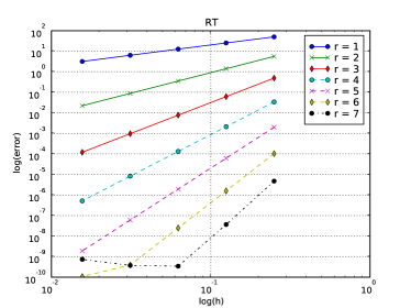
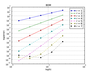
Fig. 4: Convergence rates for the discretized mixed Poisson equation (1) using $\mathrm{RT}_{r-1}\times\mathrm{DG}_{r-1}$ (left) and $\mathrm{BDM}_{r}\times DG_{r-1}$ (right), $r=1,2,\ldots,7$. Logarithmic plots of the $L^{2}$ error of the flux approximation: $||\sigma-\sigma_{h}||_{0}$ versus mesh size. The convergence rates in the left plot are $\mathcal{O}(h^{r})$ and the convergence rates in the right plot are $\mathcal{O}(h^{r+1})$; cf. Table 2. The error does not converge below $\sim 10^{-10}$ in our experiments as a result of limited precision in the evaluation of integrals and/or linear solvers. The exact source of the limited precision has not been investigated in detail.

Table 5: Averaged convergence rates for the discretized curl-div formulation of the Hodge Laplace equation (3) using $\mathrm{NED}_{r-1}\times\mathrm{RT}_{r-1}$, $r=1,2,3$, and $\mathrm{NED}_{r}\times\mathrm{BDM}_{r}$, $r=1,2$. Number of degrees of freedom in the range $80{,}000$–$300{,}000$.

Element	$||\sigma-\sigma_{h}||_{0}$	$||\sigma-\sigma_{h}||_{\operatorname{curl}}$	$||u-u_{h}||_{0}$	$||u-u_{h}||_{\operatorname{div}}$
$\mathrm{NED}_{0}\times\mathrm{RT}_{0}$	0.99	0.98	0.99	0.98
$\mathrm{NED}_{1}\times\mathrm{BDM}_{1}$	1.96	2.00	1.95	0.96
$\mathrm{NED}_{1}\times\mathrm{RT}_{1}$	1.97	1.97	1.98	1.98
$\mathrm{NED}_{2}\times\mathrm{BDM}_{2}$	3.00	2.99	2.97	1.97
$\mathrm{NED}_{2}\times\mathrm{RT}_{2}$	2.98	2.96	2.97	2.97

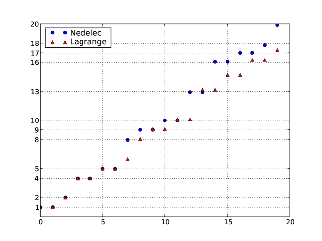
Fig. 5: The first $20$ eigenvalues of the cavity resonator problem computed using first order Nédélec elements ($\mathrm{NED}_{0}$) and Lagrange elements ($P_{1}$) on a coarse ($16\times 16$) criss-cross mesh. The exact analytical values are indicated by the horizontal grid lines.

by the Nédélec edge elements on a regular criss-cross triangulation are given in comparison with the corresponding Lagrange eigenvalue approximations $\omega^{2}_{h,L}$. Note the treacherous spurious Lagrange approximations such as $\omega^{2}_{h,L}\approx 6,15$.

6.3 Elasticity with weakly imposed symmetry

As a final example, we consider a mixed finite element formulation of the equations of linear elasticity with the symmetry of the stress tensor imposed weakly as given in Example 2.4. In the homogeneous, isotropic case, the inner product induced by the compliance tensor $A$ reduces to

$$\langle\tau,A\sigma\rangle=\nu\langle\tau,\sigma\rangle-\zeta\langle\operatorname{tr}\tau,\operatorname{tr}\sigma\rangle$$

for $\nu,\zeta$ material parameters. A stable family of finite element spaces for the discretization of (6) is given by [6]: $\mathrm{BDM}^{2}_{r}\times\mathrm{DG}^{2}_{r-1}\times\mathrm{DG}_{r-1}\subset H(\operatorname{div};\Omega,\mathbb{M})\times L^{2}(\Omega,\mathbb{R}^{n})\times L^{2}(\Omega)$, $r=1,2,\dots$. The $17$ lines of FFC code sufficient to define this discretization are included in Table 6.

Again to demonstrate convergence, we consider a regular triangulation of the unit square and solve for the smooth solution

(30) $$u(x_{0},x_{1})=\begin{pmatrix}-x_{1}\sin(\pi x_{0})\\ 0.5\pi x_{1}^{2}\cos(\pi x_{0})\end{pmatrix}.$$

The theoretically predicted convergence rate of the discretization introduced above is of the order $\mathcal{O}(h^{r})$ for all computed quantities. The numerical experiments corroborate this prediction. In particular, the convergence of the stress approximation in the $H(\mathrm{div})$ norm can be examined in Figure 6.

Table 6: FFC code for linear elasticity with weak symmetry.

def A(sigma, tau, nu, zeta): return (nu*dot(sigma, tau) - zeta*trace(sigma)*trace(tau))*dx def b(tau, w, eta): return (div(tau[0])*w[0] + div(tau[1])*w[1] + skew(tau)*eta)*dx nu = 0.5 zeta = 0.2475 r = 2 S = FiniteElement("BDM", "triangle", r) V = VectorElement("Discontinuous Lagrange", "triangle", r-1) Q = FiniteElement("Discontinuous Lagrange", "triangle", r-1) MX = MixedElement([S, S, V, Q]) (tau0, tau1, v, eta) = TestFunctions(MX) (sigma0, sigma1, u, gamma) = TrialFunctions(MX) sigma = [sigma0, sigma1] tau = [tau0, tau1] a = A(sigma, tau, nu, zeta) + b(tau, u, gamma) + b(sigma, v, eta) L = dot(v, f)*dx

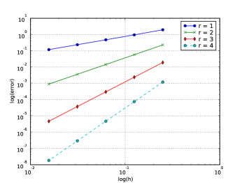
Fig. 6: Left: Convergence rates for elastic stress approximations of (6). Logarithmic plot of $H(\mathrm{div})$ error of the approximated stress $\sigma$ versus mesh size. The convergence rates are $\mathcal{O}(h^{r})$, $r=1,2,3,4$. Right: Elastic dolphin hanging by the tail under a gravitational force.

7 Conclusions

The relative scarcity of $H(\mathrm{div})$ and $H(\mathrm{curl})$ mixed finite element formulations in practical use may be attributed to their higher theoretical and implementational threshold. Indeed, more care is required to implement their finite element basis functions than the standard Lagrange bases, and assembly poses additional difficulties. However, as demonstrated in this work, the implementation of mixed finite element formulations over $H(\mathrm{div})$ and $H(\mathrm{curl})$ may be automated and thus be used with the same ease as standard formulations over $H^{1}$. In particular, the additional challenges in the assembly can be viewed as not essentially different from those encountered when assembling higher order Lagrange elements.

The efficiency of the approach has been further investigated by Ølgaard and Wells [32], with particular emphasis on the performance when applied to more complicated PDEs. They conclude that the tensor representation significantly improves performance for forms below a certain complexity level, corroborating the previous results of [21]. However, an automated, optimized quadrature approach, also supported by FFC, may prove significantly better for more complex forms. These findings indicate that a system for automatically detecting the better approach may be valuable.

The tools (FFC, FIAT, DOLFIN) used to compute the results presented here are freely available as part of the FEniCS project [15] and it is our hope that this may contribute to further the use of mixed formulations in applications.

References

- [1] FEAP: A Finite Element Analysis Program, http://www.ce.berkeley.edu/projects/feap/.
- [2] M. Ainsworth and J. Coyle, Hierarchic finite element bases on unstructured tetrahedral meshes, Internat. J. Numer. Methods Engrg., 58 (2003), pp. 2103–2130.
- [3] M. Alnæs, A. Logg, K.-A. Mardal, O. Skavhaug, and H. P. Langtangen, UFC Specification and User Manual 1.1, http://www.fenics.org/ufc/ (2008).
- [4] D. N. Arnold, D. Boffi, and R. S. Falk, Quadrilateral finite elements, SIAM J. Numer. Anal., 42 (2005), pp. 2429–2451.
- [5] D. N. Arnold, R. S. Falk, and R. Winther, Finite element exterior calculus, homological techniques, and applications, Acta Numer., 15 (2006), pp. 1–155.
- [6] D. N. Arnold, R. S. Falk, and R. Winther, Mixed finite element methods for elasticity with weakly imposed symmetry, Math. Comp., 76 (2007), pp. 1699–1723.
- [7] D. N. Arnold and R. Winther, Mixed finite elements for elasticity, Numer. Math., 92 (2002), pp. 401–419.
- [8] W. Bangerth, R. Hartmann, and G. Kanschat, deal.II Differential Equations Analysis Library, http://www.dealii.org/ (2006).
- [9] F. Brezzi, J. Douglas, Jr., M. Fortin, and L. D. Marini, Efficient rectangular mixed finite elements in two and three space variables, RAIRO Modél. Math. Anal. Numér., 21 (1987), pp. 581–604.
- [10] F. Brezzi, J. Douglas, Jr., and L. D. Marini, Two families of mixed finite elements for second order elliptic problems, Numer. Math., 47 (1985), pp. 217–235.
- [11] F. Brezzi and M. Fortin, Mixed and Hybrid Finite Element Methods, Springer Ser. Comput. Math. 15, Springer-Verlag, New York, 1991.
- [12] P. Castillo, R. Rieben, and D. White, FEMSTER: An object-oriented class library of high-order discrete differential forms, ACM Trans. Math. Software, 31 (2005), pp. 425–457.
- [13] P. G. Ciarlet, Numerical Analysis of the Finite Element Method, Sémin. Math. Supér. 59, Les Presses de l’Université de Montréal, Montreal, 1976.
- [14] V. Domínguez and F.-J. Sayas, Algorithm : A simple Matlab implementation of the Argyris element, ACM Trans. Math. Software, 35 (2009), 11 pp.
- [15] J. Hoffman, J. Jansson, C. Johnson, M. G. Knepley, R. C. Kirby, A. Logg, L. R. Scott, and G. N. Wells, FEniCS, http://www.fenics.org/ (2006).
- [16] R. C. Kirby, Algorithm : FIAT, a new paradigm for computing finite element basis functions, ACM Trans. Math. Software, 30 (2004), pp. 502–516.
- [17] R. C. Kirby, FIAT, http://www.fenics.org/fiat/ (2006).
- [18] R. C. Kirby, Optimizing FIAT with Level BLAS, ACM Trans. Math. Software, 32 (2006), pp. 223–235.
- [19] R. C. Kirby, M. Knepley, A. Logg, and L. R. Scott, Optimizing the evaluation of finite element matrices, SIAM J. Sci. Comput., 27 (2005), pp. 741–758.
- [20] R. C. Kirby and A. Logg, A compiler for variational forms, ACM Trans. Math. Software, 32 (2006), pp. 417–444.
- [21] R. C. Kirby and A. Logg, Efficient compilation of a class of variational forms, ACM Trans. Math. Software, 33 (2007), 20 pp.
- [22] R. C. Kirby and A. Logg, Benchmarking domain-specific compiler optimizations for variational forms, ACM Trans. Math. Software, 35 (2008), 18 pp.
- [23] R. C. Kirby, A. Logg, L. R. Scott, and A. R. Terrel, Topological optimization of the evaluation of finite element matrices, SIAM J. Sci. Comput., 28 (2006), pp. 224–240.
- [24] R. C. Kirby and L. R. Scott, Geometric optimization of the evaluation of finite element matrices, SIAM J. Sci. Comput., 29 (2007), pp. 827–841.
- [25] A. Logg, FFC, http://www.fenics.org/ffc/ (2006).
- [26] A. Logg, Automating the finite element method, Arch. Comput. Methods Eng., 14 (2007), pp. 93–138.
- [27] K. A. Mardal, X.-C. Tai, and R. Winther, A robust finite element method for Darcy–Stokes flow, SIAM J. Numer. Anal., 40 (2002), pp. 1605–1631.
- [28] P. Monk, Finite Element Methods for Maxwell’s Equations, Oxford University Press, New York, 2003.
- [29] J.-C. Nédélec, Mixed finite elements in , Numer. Math., 35 (1980), pp. 315–341.
- [30] J.-C. Nédélec, New mixed finite elements in , Numer. Math., 50 (1986), pp. 57–81.
- [31] K. B. Ølgaard, A. Logg, and G. N. Wells, Automated code generation for discontinuous Galerkin methods, SIAM J. Sci. Comput., 31 (2008), pp. 849–864.
- [32] K. B. Ølgaard and G. N. Wells, Optimisations for quadrature representations of finite element tensors through automated code generation, ACM Trans. Math. Software, to appear.
- [33] O. Pironneau, F. Hecht, A. L. Hyaric, and K. Ohtsuka, FreeFEM, http://www.freefem.org/ (2006).
- [34] P.-A. Raviart and J. M. Thomas, Primal hybrid finite element methods for nd order elliptic equations, Math. Comp., 31 (1977), pp. 391–413.
- [35] A. Schneebeli, An Conforming FEM: Nédélec’s Element of the First Type, Technical report, 2003; also available online from http://www.dealii.org/developer/reports/ nedelec/nedelec.pdf.
- [36] J. Schöberl, NGSolve, http://www.hpfem.jku.at/ngsolve/index.html/ (2008).