Towards Conformal Invariance
and a Geometric Representation
of the 2D Ising Magnetization Field

Abstract

We study the continuum scaling limit of the critical Ising magnetization in two dimensions. We prove the existence of subsequential limits, discuss connections with the scaling limit of critical FK clusters, and describe work in progress of the author with C. Garban and C.M. Newman.

Keywords: continuum scaling limit, critical and near/off-critical Ising model, Euclidean field theory, FK clusters.

AMS 2000 Subject Classification: 82B27, 60K35, 82B43, 60D05.

1 Synopsis

The Ising model in $d=2$ dimensions is perhaps the most studied statistical mechanical model and has a special place in the theory of critical phenomena since the groundbreaking work of Onsager [29]. Its scaling limit at or near the critical point is recognized to give rise to Euclidean (quantum) field theories. In particular, at the critical point, the lattice magnetization field should converge, in the scaling limit, to a Euclidean random field $\Phi^{0}$ corresponding to the simplest reflection-positive conformal field theory [3, 12]. As such, there have been a variety of representations in terms of free fermion fields [34] and explicit formulas for correlation functions (see, e.g., [24, 30] and references therein).

In [11], C.M. Newman and the present author introduced a representation of $\Phi^{0}$ in terms of random geometric objects associated with Schramm-Loewner Evolutions (SLEs) [33] (see also [13, 22, 23, 41]) and Conformal Loop Ensembles (CLEs) [36, 42, 37, 38]—namely, a gas (or random process) of continuum loops and associated clusters and (renormalized) area measures.

The purpose of the present paper is twofold, as we now explain. First of all, we provide a detailed proof of the existence of subsequential limits of the lattice magnetization field as a square integrable random variable and a random generalized function (Theorem 1) following the ideas presented in [11]. We also introduce a cutoff field whose scaling limit admits a geometric representation in terms of rescaled counting measures associated to critical FK clusters, and show that it converges to the magnetization field as the cutoff is sent to zero (Theorem 2).

Secondly, we describe work in progress [7] of the author with C. Garban and C.M. Newman aimed at establishing uniqueness of the scaling limit of the lattice magnetization and conformal covariance properties for the limiting magnetization field. We also explain how the existence and conformal covariance properties of the magnetization field should imply the convergence, in the scaling limit, of a version of the model with a vanishing (in the limit) external magnetic field to a field theory with exponential decay of correlations, and how they can be used to determine the free energy density of the model up to a constant (equation (11)).

2 The Magnetization and Some Results

We consider the standard Ising model on the square lattice ${\mathbb{Z}}^{2}$ with (formal) Hamiltonian

$${\bf H}=-\sum_{\{x,y\}}S_{x}S_{y}-H\sum_{x}S_{x}\,,$$ (1)

where the first sum is over nearest-neighbor pairs in ${\mathbb{Z}}^{2}$, the spin variables $S_{x},S_{y}$ are $(\pm 1)$-valued and the external field $H$ is in $\mathbb{R}$. For a bounded $\Lambda\subset{\mathbb{Z}}^{2}$, the Gibbs distribution is given by $\frac{1}{Z_{\Lambda}}\,e^{-\beta\,{\bf H}_{\Lambda}}$, where ${\bf H}_{\Lambda}$ is the Hamiltonian (1) with sums restricted to sites in $\Lambda$, $\beta\geq 0$ is the inverse temperature, and the partition function $Z_{\Lambda}$ is the appropriate normalization needed to obtain a probability distribution.

We are mostly interested in the model with zero (or vanishing) external field, and at the critical inverse temperature, $\beta_{c}=\frac{1}{2}\,\log{(1+\sqrt{2})}$. For all $\beta\leq\beta_{c}$, the model has a unique infinite-volume Gibbs distribution for any value of the external field $H$, obtained as a weak limit of the Gibbs distribution for bounded $\Lambda$ by letting $\Lambda\uparrow{\mathbb{Z}}^{2}$. For any value of $\beta\leq\beta_{c}$ and of $H$, expectation with respect to the unique infinite-volume Gibbs distribution will be denoted by $\langle\cdot\rangle_{\beta,H}$. At the critical point, that is when $\beta=\beta_{c}$ and $H=0$, expectation will be denoted by $\langle\cdot\rangle_{c}$. By translation invariance, the two-point correlation $\langle S_{x}S_{y}\rangle_{\beta,H}$ is a function only of $y-x$, which at the critical point we denote by $\tau_{c}(y-x)$.

We want to study the random field associated with the spins on the rescaled lattice $a\,{\mathbb{Z}}^{2}$ in the scaling limit $a\to 0$. More precisely, for functions $f$ of bounded support on ${\mathbb{R}}^{2}$, we define for the critical model

$$\Phi^{a}(f)\equiv\int_{{\mathbb{R}}^{2}}f(z)\Phi^{a}(z)dz\equiv\int_{{\mathbb{R}}^{2}}f(z)[\Theta_{a}\sum_{x\in{\mathbb{Z}}^{2}}S_{x}\delta(z-ax)]dz=\Theta_{a}\sum_{z\in a\,{\mathbb{Z}}^{2}}f(z)S_{z/a}\,,$$ (2)

with scale factor

$$\Theta_{a}^{-1}\equiv\sqrt{\sum_{z,w\in\Lambda_{1,a}}\langle S_{z/a}S_{w/a}\rangle_{c}}=\sqrt{\sum_{x,y\in\Lambda_{1/a}}\tau_{c}(y-x)}\,,$$ (3)

where $\Lambda_{L,a}\equiv[0,L]^{2}\cap a\,{\mathbb{Z}}^{2}$ and $\Lambda_{L}\equiv\Lambda_{L,1}=[0,L]^{2}\cap{\mathbb{Z}}^{2}$.

The block magnetization, $M^{a}\equiv\Phi^{a}({\bf 1}_{[0,1]^{2}})$, where $\bf 1$ denotes the indicator function, is a rescaled sum of identically distributed, dependent random variables. In the high temperature case, $\beta<\beta_{c}$, and with zero external field, $H=0$, the dependence is sufficiently weak for the block magnetization to converge, as $a\to 0$, to a mean-zero, Gaussian random variable (see, e.g., [27] and references therein). In that case, the appropriate scaling factor $\Theta_{a}$ is of order $a$, and the field converges to Gaussian white noise as $a\to 0$ (see, e.g., [27]). In the critical case, however, correlations are much stronger and extend to all length scales, so that one does not expect a Gaussian limit. A proof of this will be presented elsewhere [7]; in this paper we are concerned with the existence of subsequential limits for the lattice magnetization field, and their geometric representation in terms of area measures of critical FK clusters.

The FK representation of the Ising model with zero external field, $H=0$, is based on the $q=2$ random-cluster measure $P_{p}$ (see [20] for more on the random-cluster model and its connection to the Ising model). A spin configuration distributed according to the unique infinite-volume Gibbs distribution with $H=0$ and inverse temperature $\beta\leq\beta_{c}$ can be obtained in the following way. Take a random-cluster (FK) bond configuration on the square lattice distributed according to $P_{p}$ with $p=p(\beta)=1-e^{-2\beta}$, and let $\{{\cal C}_{i}\}$ denote the corresponding collection of FK clusters, where a cluster is a maximal set of sites of the square lattice connected via bonds of the FK bond configuration (see Figure 1). One may regard the index $i$ as taking values in the natural numbers, but it’s better to think of it as a dummy countable index without any prescribed ordering, like one has for a Poisson point process. Let $\{\eta_{i}\}$ be ($\pm 1$)-valued, i.i.d., symmetric random variables, and assign $S_{x}=\eta_{i}$ for all $x\in{\cal C}_{i}$; then the collection $\{S_{x}\}_{x\in{\mathbb{Z}}^{2}}$ of spin variables is distributed according to the unique infinite volume Gibbs distribution with $H=0$ and inverse temperature $\beta$. When $\beta=\beta_{c}$, we will use the notation $P_{c}\equiv P_{p(\beta_{c})}$, and $E_{c}$ for expectation with respect to $P_{c}$.

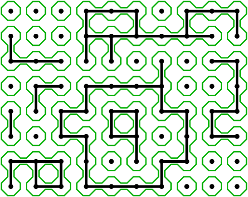
Figure 1: Example of an FK bond configuration in a rectangular region. Black dots represent sites of ${\mathbb{Z}}^{2}$, black horizontal and vertical edges represent FK bonds. The FK clusters are highlighted by lighter (green) loops on the medial lattice.

A useful property of the FK representation is that, when $H=0$, the Ising two-point function can be written as

$$\langle S_{x}S_{y}\rangle_{\beta,0}=P_{p(\beta)}(x\text{ and }y\text{ belong to the same FK cluster }{\cal C}_{i})\,.$$

As an immediate consequence, we have

$$\Theta^{-2}_{a}=\sum_{x,y\in\Lambda_{1/a}}\tau_{c}(y-x)=\sum_{x,y\in\Lambda_{1/a}}E_{c}\left[\sum_{i}{\bf 1}_{x\in{\cal C}_{i}}{\bf 1}_{y\in{\cal C}_{i}}\right]=E_{c}\left[\sum_{i}|\hat{\cal C}^{a}_{i}|^{2}\right]\,,$$ (4)

where $\hat{\cal C}^{a}_{i}$ is the restriction of the rescaled cluster ${\cal C}^{a}_{i}=a\,{\cal C}_{i}$ in $a\,{\mathbb{Z}}^{2}$ to $[0,1]^{2}$, and $|\hat{\cal C}^{a}_{i}|$ is the number of ($a\,{\mathbb{Z}}^{2}$)-sites in $\hat{\cal C}^{a}_{i}$. (Note that $\hat{\cal C}^{a}_{i}$ need not be connected.) Using the FK representation, we can write (2) as

$$\Phi^{a}(f)\stackrel{{\scriptstyle dist.}}{{=}}\sum_{i}\eta_{i}\mu^{a}_{i}(f)\,,$$ (5)

where $\mu^{a}_{i}\equiv\Theta_{a}\sum_{x\in{\cal C}_{i}}\delta(z-ax)$ and the $\eta_{i}$’s, as before, are $(\pm 1)$-valued, symmetric random variables independent of each other and everything else. We can now easily see that $\Theta_{a}$ was chosen so that the second moment of the block magnetization $M^{a}$, defined earlier, is exactly one:

$$\left\langle\left(M^{a}\right)^{2}\right\rangle_{c}=\left\langle\left[\Phi^{a}({\bf 1}_{[0,1]^{2}})\right]^{2}\right\rangle_{c}=E_{c}\left[\sum_{i}\left(\mu^{a}_{i}({\bf 1}_{[0,1]^{2}})\right)^{2}\right]=\Theta^{2}_{a}E_{c}\left[\sum_{i}|\hat{\cal C}^{a}_{i}|^{2}\right]=1\,.$$ (6)

We can associate in a unique way to each rescaled counting measure $\mu^{a}_{i}$ the interface $\gamma^{a}_{i}$ in the medial lattice between the corresponding (rescaled) FK cluster ${\cal C}^{a}_{i}$ and the surrounding FK clusters. Since all FK clusters are almost surely finite at the critical point ($\beta=\beta_{c},H=0$), such interfaces form closed curves, or loops, which separate the corresponding clusters ${\cal C}^{a}_{i}$ from infinity (see Fig. 1). There are two types of loops: (1) those with sites of $a\,{\mathbb{Z}}^{2}$ immediately on their inside and (2) those with sites of $a\,{\mathbb{Z}}^{2}$ immediately on their outside. We denote by $\{\gamma^{a}_{i}\}$ the (random) collection of all loops of the first type associated with the FK clusters $\{{\cal C}^{a}_{i}\}$. Each realization of $\{\gamma^{a}_{i}\}$ can be seen as an element in a space of collections of loops with the Aizenman-Burchard metric [2]. (The latter is the induced Hausdorff metric on collections of curves associated to the metric on curves given by the infimum over monotone reparametrizations of the supremum norm.) It follows from [2] and the RSW-type bounds of [14] (see Section 5.3 there) that, as $a\to 0$, $\{\gamma^{a}_{i}\}$ has subsequential limits in distribution to random collections of loops in the Aizenman-Burchard metric. In the scaling limit, one gets collections of nested loops that can touch (themselves and each other), but never cross.

In order to study the magnetization field, we introduce some more notation. Let $(C_{0}({\mathbb{R}}^{2}),||\cdot||_{\infty})$ denote the space of continuous functions on ${\mathbb{R}}^{2}$ with compact support, endowed with the metric of uniform convergence. Let $({\cal P}_{2},W_{2})$ denote the space of probability distributions on $\mathbb{R}$ (with the Borel $\sigma$-algebra) with finite second moment, endowed with the Wasserstein (or minimal $L_{2}$) metric

$$W_{2}(P,Q)\equiv\left(\inf E\left[|X-Y|^{2}\right]\right)^{1/2}\,,$$ (7)

where $X$ and $Y$ are coupled random variables with respective distributions $P$ and $Q$, $E$ denotes expectation with respect to the coupling, and the infimum is taken over all such couplings (see, e.g., [31] and references therein). Convergence in the Wasserstein metric $W_{2}$ is equivalent to convergence in distribution plus convergence of the second moment. For brevity, we will write $C_{0}({\mathbb{R}}^{2})$ and ${\cal P}_{2}$, instead of $(C_{0}({\mathbb{R}}^{2}),||\cdot||_{\infty})$ and $({\cal P}_{2},W_{2})$, unless we wish to emphasize the role of the metrics.

We further denote by ${\cal D}$ the space of infinitely differentiable functions on ${\mathbb{R}}^{2}$ with compact support, equipped with the topology of uniform convergence of all derivatives, and by ${\cal D}^{\prime}$ its topological dual, i.e., the space of all generalized functions.

The next theorem shows that the lattice magnetization field has subsequential scaling limits in terms of continuous functionals, in a distributional sense using the Wasserstein metric $W_{2}$, and in the sense of generalized functions by an application of the Bochner-Minlos theorem. (We remark that the last statement of Theorem 1 is not optimal in the sense that similar conclusions should apply to a larger class of functions than $\cal D$.)

Theorem 1.

For any sequence $a_{n}\to 0$, there exists a subsequence $a_{n_{k}}\to 0$ such that, for all $f\in C_{0}({\mathbb{R}}^{2})$, the distribution $P^{k}_{f}$ of $\Phi^{a_{n_{k}}}(f)$ converges in the Wasserstein metric (7), as $k\to\infty$, to a limit $P^{0}_{f}\in{\cal P}_{2}$ such that the map $P^{0}_{\cdot}:(C_{0}({\mathbb{R}}^{2}),||\cdot||_{\infty})\longrightarrow({\cal P}_{2},W_{2})$ is continuous. Furthermore, for every subsequential limit $P^{0}_{\cdot}$, there exists a random generalized function $\Phi^{0}\in{\cal D}^{\prime}$ with characteristic function $\chi(f)\equiv\int e^{ix}dP^{0}_{f}(x)$.

Theorem 1 represents the starting point of a joint project with C. Garban and C.M. Newman aimed at establishing uniqueness of the scaling limit of the lattice magnetization field and its conformal covariant properties. One not only expects a unique scaling limit for the lattice magnetization field, but based on the representation (5), one would like to write the limiting field $\Phi^{0}$ as

$$``\Phi^{0}(f)=\sum_{j}\eta_{j}\mu^{0}_{j}(f)"$$ (8)

where the $\mu^{0}_{j}(f)$’s are the putative scaling limits of the $\mu^{a}_{i}(f)$’s that appear in (5). Indeed, in the scaling limit, one should obtain a collection $\{\mu^{0}_{j}\}$ of mutually orthogonal, finite measures supported on the scaling limit of the critical FK clusters. However, due to scale invariance, $\{\mu^{0}_{j}\}$ should contain (countably) infinitely many elements, and the scaling covariance expected for the $\mu^{0}_{j}$’s suggests that the collection $\{\mu^{0}_{j}(f)\}$ is in general not absolutely summable. What meaning, if any, can we then attribute to the sum in (8)?

To help answer that question, we introduce the $\varepsilon$-cutoff lattice magnetization field

$$\Phi^{a}_{\varepsilon}(f)\equiv\sum_{i:diam({\gamma}^{a}_{i})>\varepsilon}\eta_{i}\mu^{a}_{i}(f)\,,$$ (9)

where the elements of the collection $\{\mu^{a}_{i}\}$ of all rescaled (random) measures that are involved in (9) are those associated to rescaled FK clusters ${\cal C}^{a}_{i}$ that intersect the support of $f$ and whose corresponding loops $\gamma^{a}_{i}$ have diameter $>\varepsilon$.

Once again, one would like to write the scaling limit of the cutoff field as “$\Phi^{0}_{\varepsilon}(f)=\sum_{j:diam({\gamma}^{0}_{j})>\varepsilon}\eta_{j}\mu^{0}_{j}(f)$”. In this case however, the sum would be unambiguous because it would contain only a finite number of terms. A proof of the latter fact follows from Prop. 5.1 in Section 5. Combined with (6) and Prop. 6.2 in Section 6, Prop. 5.1 implies that the collection of $\mu^{a}_{i}(f)$’s corresponding to macroscopic FK clusters has nontrivial subsequential scaling limits. Indeed, it is clear from equation (6) that no $\mu^{a}_{i}({\bf 1}_{[0,1]^{2}})$ can diverge as $a\to\infty$. In addition, Prop. 6.2 says that “small” FK clusters do not contribute to the magnetization in the scaling limit and thus, by Prop. 5.1, the number of FK clusters which contribute significantly to $M^{a}=\Phi^{a}({\bf 1}_{[0,1]^{2}})$ remains bounded as $a\to 0$. Since $\left\langle(M^{a})^{2}\right\rangle_{c}=1$ for all $a$, this implies that not all $\mu^{a}_{i}({\bf 1}_{[0,1]^{2}})$’s can converge to 0 as $a\to 0$. Prop. 6.1 ensures that the same conclusions hold not only for the collection of $\mu^{a}_{i}(f)$’s with $f={\bf 1}_{[0,1]^{2}}$, but for other functions as well.

The result below shows that, in the scaling limit, one recovers the “full” magnetization field from the cutoff one by letting the cutoff go to zero.

Theorem 2.

For any sequence $a_{n}\to 0$, there exists a subsequence $a_{n_{k}}\to 0$ such that, for all $f\in C_{0}({\mathbb{R}}^{2})$ and all $m\in{\mathbb{N}}$, the distributions of $\Phi^{a_{n_{k}}}(f)$ and $\Phi^{a_{n_{k}}}_{1/m}(f)$ converge in the Wasserstein metric (7) as $k\to\infty$. Moreover, if $P^{0}_{f}$ and $P^{0}_{f,m}$ denote the respective limits, $P^{0}_{f,m}$ converges to $P^{0}_{f}$ in the Wasserstein metric (7) as $m\to\infty$.

In view of Theorem 2, one can interpret the sum in equation (8) as a shorthand for the limit of the cutoff field as the cutoff is removed. Combined with the fact that the collection of $\mu^{a}_{i}(f)$’s has nontrivial subsequential scaling limits, as explained above, Theorems 1 and 2 partly establish the geometric representation proposed in [11]. In order to establish the existence of a unique scaling limit for the collection of $\mu^{a}_{i}$’s as measures, and to obtain their conformal covariance properties and those of the limiting magnetization field $\Phi^{0}$, more work is needed. This is discussed in the next section.

3 Work in Progress: Uniqueness and Conformal Covariance

The lattice magnetization field is expected to have a unique scaling limit $\Phi^{0}$ with the property of transforming covariantly under conformal transformations, i.e., if $\varphi$ is a conformal map,

$$\Phi^{0}(\varphi(z))\stackrel{{\scriptstyle dist.}}{{=}}|\varphi^{\prime}(z)|^{-1/8}\Phi^{0}(z)\,,$$ (10)

where $1/8$ is the Ising magnetization exponent. (With an abuse of notation, we identify ${\mathbb{R}}^{2}$ and the complex plane $\mathbb{C}$.)

It is natural to attempt to prove such results using announced results for FK percolation (see [39, 40]) which identify the scaling limit of the FK cluster boundaries (see Fig. 1) with SLE-type random fractal curves whose distribution is invariant under conformal transformations. In order to exploit such results, one can use techniques developed in [17, 16] to study the scaling limit of Bernoulli and dynamical percolation in two dimensions. Roughly speaking, the idea is to prove that the scaling limit of the ensemble $\{\mu^{a}_{i}\}$ of rescaled counting measures associated to the FK clusters is a measurable function of the collection of limiting (macroscopic) loops between FK clusters.

To illustrate the idea, we take a small detour and discuss briefly the scaling limit of Bernoulli percolation, focusing on site percolation on the triangular lattice. The “full” scaling limit of percolation, comprising all interface loops separating macroscopic clusters, was obtained by Camia and Newman in [8, 9] and shown to be a (nested) Conformal Loop Ensemble (CLE) in [10]. In [5, 6] Camia, Fontes and Newman proposed to construct the near/off-critical scaling limit of percolation, with density of open sites $p=1/2+\lambda a^{3/4}$ (where $\lambda\in(-\infty,\infty)$ is a parameter, $a$ the lattice spacing, and $3/4$ the percolation correlation length exponent), from the critical one “augmented” by a “Poissonian cloud” of marks on the double points of the limiting loops (i.e., where a loop touches itself or where two different loops touch each other). Back on the lattice, the marked points would correspond to “pivotal” sites that switch state when the density of open sites is changed from $1/2$ to $p$, causing a macroscopic change in connectivity. (The last sentence should be interpreted in the context of the canonical coupling of percolation models at different densities of open sites. In this coupling, a percolation model with density $p$ of open sites is obtained by assigning independent, uniform random variables $u_{x}\in[0,1]$ to the sites $x$ of the lattice, and declaring open all sites with $u_{x}<p$, and closed all other sites.) A key step in the implementation of this idea is the construction of the intensity measure of the Poisson process of marks. Since the points to be marked are double points, it was argued in [5, 6] that the intensity measure should arise as the scaling limit of the appropriately rescaled counting measure of $\varepsilon$-macroscopically pivotal sites on the lattice with spacing $a$, where an $\varepsilon$-macroscopically pivotal site $x$ has four neighbors which are the starting points of four alternating paths, two made of (nearest-neighbor) open sites and two of closed ones, reaching a distance $\varepsilon$ away from $x$.

The occurrence of an $\varepsilon$-macroscopically pivotal site $x$ in a percolation configuration is called a four-arm event. The scaling limit of the counting measure of $\varepsilon$-macroscopically pivotal sites was obtained by Garban, Pete and Schramm [17] (see also [16]) and used by the same authors, in the spirit of the program proposed by Camia, Fontes and Newman, to construct the near/off-critical scaling limit of percolation. In particular, Garban, Pete and Schramm [17] consider the joint distribution of the collection of interface loops and the (random) counting measure of $\varepsilon$-macroscopically pivotal sites, $(\{\gamma^{a}_{i}\},\lambda^{a}_{\varepsilon})$, and show that it converges to the law of some random variable $(\{\gamma_{j}^{0}\},\lambda^{0}_{\varepsilon})$, where $\{\gamma_{j}^{0}\}$ is the collection of limiting loops and $\lambda^{0}_{\varepsilon}$ is a random Borel measure. Moreover, they show that $\lambda^{0}_{\varepsilon}$ is a measurable function of $\{\gamma_{j}^{0}\}$.

This last observation is in fact crucial, since the known uniqueness of the scaling limit of the interface loops implies the uniqueness of $\lambda^{0}_{\varepsilon}$. In addition, one can deduce how $\lambda^{0}_{\varepsilon}$ changes under conformal transformations from the knowledge of how $\{\gamma_{j}^{0}\}$ changes under those same transformations. The latter can be deduced for the collection $\{\gamma_{j}^{0}\}$ from the fact that it is a nested CLE whose loops are SLE-type curves.

Heuristically, one can convince oneself that it is reasonable to expect that $\lambda^{0}_{\varepsilon}$ be a measurable function of $\{\gamma_{j}^{0}\}$ by noticing that knowing the macroscopic loops should be sufficient to give a good estimate of the number of macroscopically pivotal sites. For a discussion on how to turn this observation into a proof, the reader is referred to Sect. 4.3 of [17], where complete proofs of the results mentioned in the previous paragraph can also be found.

In Sect. 5 of [17], the authors discuss how to obtain similar results for rescaled counting measures of other special sites. In particular, they show how to obtain what they call the “cluster” or “area” measure, which counts the number of open sites contained in clusters of diameter larger than some cutoff $\varepsilon>0$. The occurrence of such a site $x$ corresponds to the event that there is a path of (nearest-neighbor) open sites starting at $x$ and reaching a distance $\varepsilon$ away from $x$. Such an event is called a one-arm event, and we will call $x$ a one-arm site. The proof in this case is in fact simpler because the event is simpler, involving only one path.

At this point the reader should note that the area measures $\mu^{a}_{i}$ introduced in the previous section in connection with the magnetization field also count one-arm sites, with the only difference that the relevant one-arm events are now in the context of FK bond percolation. FK percolation is more difficult to analyze than Bernoulli percolation, due to the dependencies in the distribution of FK configurations (as opposed to the product measure corresponding to Bernoulli percolation). However, it seems that one can successfully adapt the techniques of [17, 16], at least for the case of one-arm sites which is relevant for the magnetization. As a consequence, thanks to the results announced in [39, 40], one should obtain uniqueness of the limiting ensemble $\{\mu^{0}_{j}\}$ of area measures for the FK clusters and of the magnetization field $\Phi^{0}$, as well as a proof of (10) and of the fact that, for any conformal map $\varphi$, $\{|\varphi^{\prime}(z)|^{-15/8}d\mu_{j}^{0}(\varphi(z))\}$ is equidistributed with $\{d\mu_{j}^{0}(z)\}$. Because of the latter property, we call the putative collection of measures $\{\mu^{0}_{j}\}$, obtained as the scaling limit of the collection of rescaled counting measures $\{\mu^{a}_{i}\}$, a Conformal Measure Ensemble.

4 More Work in Progress: Free Energy Density and Tail Behavior

The uniqueness and conformal covariance properties of $\Phi^{0}$ play an important role in the analysis of the near-critical scaling limit (called off-critical in the physics literature) with a vanishing (in the limit) external field (at the critical inverse temperature $\beta_{c}$). More precisely, consider an Ising model on $a\,{\mathbb{Z}}^{2}$ with (formal) Hamiltonian (1) and external field $H(a)=h\beta_{c}^{-1}\Theta_{a}$ inside the square $[-L,L]^{2}$, and zero outside it. We call $h$ the renormalized external field and note that the term

$$-h\beta_{c}^{-1}\Theta_{a}\sum_{z\in a\,{\mathbb{Z}}^{2}\cap[-L,L]^{2}}S_{z/a}$$

in the Hamiltonian implies that the Gibbs distribution of this particular Ising model is given by

$$d\nu_{h,L}^{a}\equiv\frac{1}{Z_{h,L}^{a}}\exp\left(h\Theta_{a}\sum_{z\in a\,{\mathbb{Z}}^{2}\cap[-L,L]^{2}}S_{z/a}\right)d\nu^{a}=\frac{1}{Z_{h,L}^{a}}\exp\left(hM^{a}_{L}\right)d\nu^{a}\,,$$

where $\nu^{a}$ is the Gibbs distribution corresponding to zero external field, $Z_{h,L}^{a}$ is the appropriate normalization factor, and $M^{a}_{L}$ denotes the block magnetization inside $[-L,L]^{2}$. As a consequence, in the scaling limit ($a\to 0$) one would obtain a distribution $\nu^{0}_{h,L}$ such that

$$d\nu^{0}_{h,L}\equiv\frac{1}{Z^{0}_{h,L}}\exp\left(h\Phi^{0}({\bf 1}_{[-L,L]^{2}})\right)d\nu^{0}\,,$$

where $Z^{0}_{h,L}\equiv\int\exp(h\Phi^{0}({\bf 1}_{[-L,L]^{2}})d\nu^{0}$ and $\nu^{0}$ is the limiting distribution corresponding to zero external field.

The question is now whether $\nu^{0}_{h,L}$ converges to some $\nu^{0}_{h}$ as $L\to\infty$, and whether $\nu^{0}_{h}$ corresponds to the physically correct near/off-critical scaling limit. Heuristically, the correct normalization to obtain a nontrivial near/off-critical scaling limit is such that the correlation length $\xi$ remains bounded away from zero and infinity. Scaling theory implies that $\xi\sim H^{-8/15}$ for small external field $H$. This gives $H\sim a^{15/8}$, which coincides with the normalization needed to obtain a nontrivial magnetization field (given by $\Theta_{a}$), as can be seen from (3) and the asymptotic behavior of $\tau_{c}$. With this in mind, we consider an Ising model on $a\,{\mathbb{Z}}^{2}$ with an external field $H=a^{15/8}$ inside $\Lambda_{L,a}$ and $0$ outside, for some large $L$. Using the two-dimensional Ising critical exponent $\delta=15$ for the magnetization (i.e., $\langle S_{0}\rangle_{\beta_{c},H}\sim H^{1/15}$ for small $H$, where $S_{0}$ denotes the spin at the origin), and denoting by $\sum_{x}^{L}$ the sum over $x$ in $\Lambda_{L/a}$, we can write the block magnetization in the unit square as

$$\frac{\langle\Theta_{a}\sum_{x}^{1}S_{x}\exp(a^{15/8}\sum_{x}^{L}S_{x})\rangle_{c}}{\langle\exp(a^{15/8}\sum_{x}^{L}S_{x})\rangle_{c}}\stackrel{{\scriptstyle L\gg 1}}{{\sim}}a^{15/8}a^{-2}\langle S_{0}\rangle_{\beta_{c},H=a^{15/8}}\sim a^{-1/8}(a^{15/8})^{1/15}=1\,.$$

Since the result is finite, this rough computation suggests a positive answer to the previous question.

Indeed, using the convergence of the lattice magnetization field to the continuum one and scaling properties of the critical FK clusters, it appears possible to show [7] that, as $L\to\infty$, $\nu^{0}_{h,L}$ has a unique weak limit, denoted by $\nu^{0}_{h}$, and that $\nu^{0}_{h}$ represents the scaling limit of the Ising model on $a\,{\mathbb{Z}}^{2}$ with external field $H(a)=h\beta_{c}^{-1}\Theta_{a}$ on the whole plane.

The idea behind a proof of this makes use of the well-known “ghost spin” representation of the Ising model with an external field, in which an additional site with spin that agrees with the external field is added and connected to all the sites of the square lattice. The external field term in the Hamiltonian can then be written (formally) as $-|H|\sum_{x}S_{x}S_{g}$, where the ghost spin $S_{g}$ is equal to the sign of the external field $H$. One can describe the Ising model with an external field using the FK representation on the new graph comprising the square lattice and the additional site carrying the ghost spin. Note however that the density of FK bonds incident on the site carrying the ghost spin is not given by $p(\beta)=1-e^{-2\beta}$, as for the other bonds, but by $1-e^{-2\beta|H|}$.

The following key observation is an easy consequence of standard properties of FK percolation. If a subset $\Lambda$ of the square lattice is surrounded by a circuit $\Gamma$ of FK bonds that belong to a cluster which also contains the site carrying the ghost spin, the FK and spin configurations in $\Lambda$ are independent of the FK and spin configurations outside the circuit $\Gamma$. The RSW-type bounds proved in [14], together with the FKG inequality [15] and scaling properties of the FK clusters and their area measures, imply that the probability to find such a circuit $\Gamma$ surrounding any bounded subset $\Lambda$ is one. This shows that the $\nu^{0}_{h,L}$-probability of any event that depends only on the restriction of the spin configuration to a finite subset $\Lambda$ of the square lattice has a limit as $L\to\infty$. Consequently, the distribution $\nu^{0}_{h,L}$ has a weak limit $\nu^{0}_{h}$ as $L\to\infty$.

It is interesting to note that the argument alluded to above also shows that $\nu^{0}_{h}$ is locally absolutely continuous with respect to the zero-field measure $\nu^{0}$. This is in contrast to the situation in two-dimensional percolation, where the critical and near-critical measures are mutually singular [28]. It should be noted, however, that the Ising analogue of that type of percolation near-critical scaling limit is to set $H=0$ and let $\beta(a)\to\beta_{c}$, rather than set $\beta=\beta_{c}$ and let $H(a)\to 0$.

One expects the near/off-critical field to be “massive” in the sense that correlations under $\nu^{0}_{h}$ should decay exponentially at large distances. To understand why this should be the case, it is again useful to resort to the ghost spin representation discussed earlier. Remember that the Ising two-point function can be expressed in terms of connectivity properties of the FK clusters (see the discussion about the FK representation preceding equation (4)). Because of that, exponential decay of correlations is equivalent to the statement that, if two sites of the square lattice, $x$ and $y$, belong to the same FK cluster ${\cal C}_{i}$, the probability that ${\cal C}_{i}$ does not contain the site carrying the ghost spin decays exponentially in the distance between $x$ and $y$. But the scaling law for the area measures, $d\mu_{j}^{0}(\alpha\,z)\stackrel{{\scriptstyle dist.}}{{=}}\alpha^{15/8}\,d\mu_{j}^{0}(z)$ for all $\alpha>0$, suggests that a macroscopic FK cluster of diameter at least $||x-y||=O(1)$ (that is, of order $a^{-1}$ in units of the lattice spacing $a$) should contain at least $O(a^{-15/8})$ sites, precisely enough to compensate for the small intensity of the external field $H\sim a^{15/8}$, which determines the probability of a cluster to contain the site carrying the ghost spin via the density, $1-e^{-2\beta|H|}$, of FK bonds connected to that site.

The exponential decay of correlations can be used to show the existence of the free energy density $f(h)$ at the critical (inverse) temperature, defined by

$$f(h)\equiv-\beta_{c}^{-1}\lim_{L\to\infty}(2L)^{-2}\log{\left(\int\exp(h\Phi^{0}({\bf 1}_{[-L,L]^{2}}))d\nu^{0}\right)}\,,$$

provided that the limit exists. (Because of symmetry, it suffices to consider positive external fields, $h\geq 0$.) For the nearest-neighbor lattice Ising model, following a standard argument (see for instance [25], Lecture 8), one can show the existence of the free energy by partitioning $[-L,L]^{2}$ into equal squares of fixed size and writing the Hamiltonian as a sum of terms of two types: those corresponding to the interactions between spins inside a square, and the boundary terms that account for the interactions between different squares. The contribution of the latter terms to the free energy vanishes in the limit $L\to\infty$ because the boundary terms grow only linearly in $L$, implying the existence of the limit defining the free energy.

In our situation, the above argument is not immediately applicable because we have already taken the scaling limit and are now dealing with a continuum model. We can however try to mimic that argument. For that purpose, we introduce the functions

$$f^{t}_{n}(h)\equiv\frac{1}{(2^{n+1})^{2}}\log{\left(\int\exp(h\Phi^{0}_{t}({\bf 1}_{[-2^{n},2^{n}]^{2}}))d\nu^{t}\right)}\,,$$

where $\Phi^{0}_{t}$ denotes the near/off-critical magnetization field with renormalized external field $t$. We now write $\Phi^{0}_{t}({\bf 1}_{[-2^{n},2^{n}]^{2}})=\sum_{k}\Phi^{0}_{t}(\text{square}_{k})$, where $\text{square}_{k}$ denotes the $k$th element in a set of equal squares of fixed size that partition $[-2^{n},2^{n}]^{2}$. Although the random variables $\Phi^{0}_{t}(\text{square}_{k})$ are clearly not independent, the exponential decay of correlations under $\nu^{t}$ implies that they are only weakly correlated when the squares are far apart, suggesting a finite limit for $f^{t}_{n}(h)$ as $n\to\infty$. One can indeed show that the exponential decay of the covariance between different squares implies that $\limsup_{n\to\infty}f^{t}_{n}(h)<\infty$. The FKG inequality easily implies that $f^{0}_{n}(h)\leq f^{t}_{n}(h)$ for $h,t\geq 0$, and that $f^{0}_{n}(h)$ and $f^{t}_{n}(h)$ are increasing in $n$. Therefore, one can conclude the existence of a finite limit for $f^{0}_{n}(h)$ as $n\to\infty$. Comparing the definitions of $f^{0}_{n}(h)$ and $f(h)$, this strongly suggests (and can be used to prove) the existence of the limit defining $f(h)$.

Integrating (10), one can check that

$$\Phi^{0}({\bf 1}_{[-\alpha L,\alpha L]^{2}})\stackrel{{\scriptstyle dist.}}{{=}}\alpha^{15/8}\,\Phi^{0}({\bf 1}_{[-L,L]^{2}})\,,$$

consistent with the scaling law for area measures. If the limit defining the free energy density exists (and is unique), the above observation implies that $f(th)/f(t)=h^{16/15}$, which means that the free energy density must take the form

$$f(h)=C_{1}\,h^{16/15}$$ (11)

for some constant $C_{1}$. An immediate consequence of (11) would be the determination of the tail behavior of the block magnetization:

$$Prob(\Phi^{0}({\bf 1}_{[0,1]^{2}})>x)\sim\exp{(-C_{2}\,x^{16})}\text{ \,\,\,\,\,\,\, for }x>0\text{ and some constant }C_{2}>0.$$

This result would follow from the methods of [26] (see, in particular, Theorem 1.4 and Corollary 2.6 there for one-sided bounds of the same type under similar conditions) and it would show, incidentally, that the scaling limit magnetization field is not Gaussian.

5 Beyond The Ising Model in Two Dimensions

In this section, we briefly discuss the applicability of the approach presented in [11] and in this paper to higher dimensions, $d>2$, and to $q$-state Potts models with $q>2$. Although the $d=2$ scaling limit Ising magnetization field $\Phi^{0}$ should transform covariantly under conformal transformations and have close connections to the Schramm-Loewner Evolution (SLE), no conformal machinery seems necessary to establish the existence of subsequential scaling limits in terms of area measures of critical FK clusters.

A main ingredient used in this paper is Prop. 6.2, which essentially says that “small” FK clusters do not contribute to the magnetization in the scaling limit. This follows from the behavior of the two-point function at long distance (Prop. 6.1). Inspecting the proof, it is easy to check that, in order for Prop. 6.2 to hold in dimension $d\geq 2$, $\tau_{c}(y-x)$ should behave at long distance like $||y-x||^{-d+2-\eta}$ with $\eta<2$ (see [11]). Such a decay for $\tau_{c}$ should be valid for all $d\geq 2$. (In particular, $\eta$ should be 0 above four dimensions, a result which has been proved when the number of dimensions is sufficiently high [21].) However, there is a significant difference between dimensions below and above $d=4$, where 4 is the upper-critical dimension for the Ising model. As we mentioned earlier, for $d=2$ the number of terms in the sum that defines the cutoff field (9) remains a.s. finite in the scaling limit. This is due to the following result, whose proof is postponed to the next section.

Proposition 5.1.

For $z\in{\mathbb{R}}^{2}$, let $N^{a}(z,r_{1},r_{2})$ denote the number of distinct clusters ${\cal C}_{i}^{a}$ that include sites in both $\{y\in a\,{\mathbb{Z}}^{2}:||y-z||<r_{1}\}$ and $\{y\in a\,{\mathbb{Z}}^{2}:||y-z||>r_{2}\}$. For any $0<r_{1}<r_{2}<\infty$, there exists $\lambda\in(0,1)$ such that for all $z\in{\mathbb{R}}^{2}$ and all small $a>0$ and any $k=1,2,\dots$,

$$P_{c}(N^{a}(z,r_{1},r_{2})\geq k)\,\leq\,\lambda^{k}\,.$$ (12)

It follows that for any bounded $D\subset{\mathbb{R}}^{2}$ and $\varepsilon>0$, the number of distinct clusters ${\cal C}_{i}^{a}$ of diameter $>\varepsilon$ touching $D$ is bounded in probability as $a\to 0$.

The analogue of Prop. 5.1 is expected to fail above the upper-critical dimension $d=4$ (see Appendix A of [1]). When it fails, there can be infinitely many FK clusters with diameter greater than $\varepsilon$ in a bounded region and so Prop. 6.2 would not preclude $\Phi^{0}$ from being a Gaussian (free) field. But it appears that at least for $d=3$, both the analogue of Prop. 5.1 and a representation of $\Phi^{0}_{\varepsilon}$ as a sum of finite measures with random signs ought to be valid.

An analogous representation for the scaling limit magnetization fields of $q$-state Potts models also ought to be valid, at least for values of $q$ such that for a given $d$, the phase transition at $\beta_{c}$ is second order. (This was pointed out to the authors of [11] by J. Cardy.) The phase transition is believed to be first order for integer $q\geq 3$ when $d\geq 3$ and for $q>4$ when $d=2$ (see [43]); this leaves, besides the Ising case, $d=2$ and $q=3$ and $4$. We denote the states or colors of the $q$-state Potts model by $1,2,\dots,q$, and recall that in the FK representation on the lattice, all sites in an FK cluster have the same color while the different clusters are colored independently with each color equally likely. In the scaling limit, there would be finite measures $\{\mu_{j}^{0,q}\}$, and the magnetization field in the color-$k$ direction would be $\sum_{j}\eta_{j}^{k}\mu_{j}^{0,q}$ with the $\eta_{j}^{k}$’s taking the value $+1$ with probability $1/q$ (for the color $k$) and the value $-1/(q-1)$ with probability $(q-1)/q$ (for any other color). For a fixed $k$ the $\eta_{j}^{k}$’s would be independent as $j$ varies, but for a fixed $j$ they would be dependent as $k$ varies because $\sum_{k}\eta_{j}^{k}=0$.

6 Proofs

The proofs of Prop. 5.1 and Prop. 6.2 below follow [11]; we include them here for completeness.

Proof of Prop. 5.1.  We define a dual FK model by inserting a bond in the dual lattice, $({\mathbb{Z}}^{2})^{*}$, whenever the corresponding dual edge is not crossed by a bond of the FK configuration on the original lattice, ${\mathbb{Z}}^{2}$.

The proof is by induction on $k$. For $k=1$, the result follows from RSW-type bounds (Theorem 1 of [14]—see [32, 35] for the original RSW) since $N^{a}(z,r_{1},r_{2})\geq 1$ is equivalent to the absence of a circuit of dual FK bonds (i.e., bonds of the dual FK model) in the $(r_{1},r_{2})$-annulus about $z$. By self-duality at the critical point, this event has the same probability as the absence of a circuit of FK bonds in the original FK model, which in turn is bounded away from one as $a\to 0$, by RSW. Now suppose $N^{a}(z,r_{1},r_{2})\geq k-1$. Then one may do an exploration of the ${\cal C}_{i}^{a}$’s that touch $\{y\in a\,{\mathbb{Z}}^{2}:||y-z||<r_{1}\}$ until $k-1$ are found that reach $\{y\in a\,{\mathbb{Z}}^{2}:||y-z||>r_{2}\}$, making sure that all cluster explorations have been fully completed without obtaining information about the outside of the clusters. At that point, the complement $D$ of some random finite $D^{c}\subset a\,{\mathbb{Z}}^{2}$ remains to be explored and the conditional random-cluster (FK) distribution in $D$ is $P_{c}^{{\partial D},F}$ with a free boundary condition on the boundary (or boundaries) between $D$ and $D^{c}$. By RSW, the $P_{c}^{{\partial D},F}$-probability of a crossing by a sequence of FK bonds in $D$ of the $(r_{1},r_{2})$-annulus is bounded above by the original $P_{c}(N^{a}(z,r_{1},r_{2})\geq 1)$. Thus we have

$$P_{c}(N^{a}(z,r_{1},r_{2})\geq k) = P_{c}(N^{a}(z,r_{1},r_{2})\geq k-1)$$

$$P_{c}(N^{a}(z,r_{1},r_{2})\geq k|\,N^{a}(z,r_{1},r_{2})\geq k-1)$$

$$= P_{c}(N^{a}(z,r_{1},r_{2})\geq k-1)\,E_{c}[P_{c}^{{\partial D},F}(N^{a}(z,r_{1},r_{2})\geq 1)]$$

$$\leq P_{c}(N^{a}(z,r_{1},r_{2})\geq k-1)\,P_{c}(N^{a}(z,r_{1},r_{2})\geq 1)$$

$$\leq \lambda^{k}\,.$$

The last claim of the proposition follows from (12) because one may choose $O([diam(\Lambda)/\varepsilon]^{2})$ points $z_{\ell}$ in ${\mathbb{R}}^{2}$ so that any ${\cal C}_{i}^{a}$ of diameter $>\varepsilon$ touching $\Lambda$ will be counted in $N^{a}(z_{\ell},\varepsilon/4,\varepsilon/2)$ for at least one $z_{\ell}$.

The next proposition corresponds to Hypothesis 1.1 of [11] (with the exponent $\theta$ there taken to be $1/8$), where it is shown how, for the critical two-dimensional Ising model, the hypothesis follows from RSW-type bounds for FK percolation. Such bounds have recently been proved in [14]. (A derivation of similar bounds, sufficient to verify Hypothesis 1.1, is also contained in [11], but it relies on the convergence of spin-cluster interfaces to $\text{CLE}_{3}$, a result that should follow from Smirnov’s work but has not been proved yet.)

Proposition 6.1.

There are constants $K_{1}>0$ and $K_{2}<\infty$ such that for any small $\varepsilon>0$ and then for any $x\in{\mathbb{Z}}^{2}$ with large Euclidean norm $||x||$,

$$K_{2}\tau_{c}(x_{\varepsilon})\,\geq\,\tau_{c}(x)\,\geq\,K_{1}\,\varepsilon^{1/4}\tau_{c}(x_{\varepsilon})\,$$ (13)

for any $x_{\varepsilon}\in{\mathbb{Z}}^{2}$ with $||x_{\varepsilon}-\varepsilon x||\leq 1/\sqrt{2}$.

Proof.  The proposition is an immediate consequence of Prop. 27 of [14].

Proposition 6.2.

For any bounded function $f$ with bounded support,

$$\lim_{\varepsilon\to 0}\limsup_{a\to 0}E_{c}\left[\sum_{i:\text{diam}(\gamma^{a}_{i})\leq\varepsilon}(\mu^{a}_{i}(f))^{2}\right]=0\,.$$

Proof.  Using Prop. 6.1, we can compare $\sum_{z^{\prime}\in\Lambda_{\varepsilon^{\prime}r}}\tau_{c}(z^{\prime})$ for small $\varepsilon^{\prime}$ as $r\to\infty$ to $\sum_{z\in\Lambda_{r}}\tau_{c}(z)$ by using the second inequality of (13) to compare each $\tau_{c}(z^{\prime})$ to the $\tau_{c}(z)$’s with $\varepsilon^{\prime}z$ in the unit length square centered on $z^{\prime}$ (so that we may take $z^{\prime}$ as $z_{\varepsilon^{\prime}}$). Since there are approximately $(1/{\varepsilon^{\prime}})^{2}$ such $z$ sites, we have that

$$\liminf_{r\to\infty}\frac{\sum_{z\in\Lambda_{r}}\tau_{c}(z)}{({\varepsilon^{\prime}})^{-7/4}\sum_{z^{\prime}\in\Lambda_{\varepsilon^{\prime}r}}\tau_{c}(z^{\prime})}\,\geq\,K_{1}\,.$$

Using this lower bound (with $r=1/2a$ and $\varepsilon^{\prime}=2\varepsilon$) and (4), and letting $D$ denote the support of $f$ and $D_{a}\equiv D\cap a\,{\mathbb{Z}}^{2}$, we have that

$$\limsup_{a\to 0}E_{c}\left[\sum_{i:\text{diam}(\gamma^{a}_{i})\leq\varepsilon}(\mu^{a}_{i}(f))^{2}\right] \leq \left(\sup_{x\in D}|f(x)|\right)^{2}\limsup_{a\to 0}\Theta_{a}^{2}\,E_{c}\left[\sum_{i:\text{diam}(\gamma^{a}_{i})\leq\varepsilon}|{\cal C}^{a}_{i}\cap D|^{2}\right]$$

$$\leq \left(\sup_{x\in D}|f(x)|\right)^{2}\limsup_{a\to 0}\frac{\sum_{z,w\in D_{a},||z-w||\leq\varepsilon}\tau_{c}(w/a-z/a)}{\sum_{x,y\in\Lambda_{1/a}}\tau_{c}(y-x)}$$

$$\leq \left(\sup_{x\in D}|f(x)|\right)^{2}\limsup_{a\to 0}\frac{K^{\prime}(1/a)^{2}\sum_{z^{\prime}\in\Lambda_{\varepsilon/a}}\tau_{c}(z^{\prime})}{K^{\prime\prime}(1/a)^{2}\sum_{z\in\Lambda_{1/(2a)}}\tau_{c}(z)}$$

$$= K^{\prime\prime\prime}\varepsilon^{7/4}\,.\,\,\,\framebox{}$$

We are now ready to prove the two theorems.

Proof of Theorem 1.  Let $D$ denote the support of $f$; in view of (6) and (13) (compare the proof of Prop. 6.2),

$$\limsup_{a\to 0}\left\langle[\Phi^{a}(f)]^{2}\right\rangle_{c} = \limsup_{a\to 0}E_{c}\left[\sum_{i}(\mu^{a}_{i}(f))^{2}\right]$$

$$\leq \left(\sup_{x\in D}|f(x)|\right)^{2}\limsup_{a\to 0}\Theta_{a}^{2}E_{c}\left[\sum_{i}|{\cal C}^{a}_{i}\cap D|^{2}\right]<\infty$$

and thus $\Phi^{a}(f)$ has subsequential limits in distribution as $a\to 0$. Boundedness of the second moment of $\Phi^{a}(f)$ and classic Ising model results (see, e.g., [27] and references therein) imply that the fourth moment of $\Phi^{a}(f)$ remains bounded as $a\to 0$. As a consequence (see, e.g., Problem 14 in Section 8.3 of [4], p. 164), any subsequential limit of $\Phi^{a}(f)$ has a finite second moment which is the limit of the second moment of $\Phi^{a}(f)$. Thus, the distribution of $\Phi^{a}(f)$ has subsequential limits in the Wasserstein metric (7) as $a\to 0$.

Since the Euclidean distance makes $[-N,N]^{2}$ a compact metric space, the space $C([-N,N]^{2})$ of continuous, real-valued functions on $[-N,N]^{2}$ with the supremum norm is separable. Every subspace of a separable metric space is separable, thus the space $C_{0}([-N,N]^{2})$ of continuous functions with compact support contained in $[-N,N]^{2}$ with the supremum norm is also separable. Any topological space which is the union of a countable number of separable subspaces is separable, which implies that $C_{0}(\mathbb{R}^{2})=\bigcup_{N\in{\mathbb{N}}}C_{0}([-N,N]^{2})$ is separable. Let $\cal G$ denote a countable, dense subset of $C_{0}(\mathbb{R}^{2})$; it is clear from the above discussion that we can choose ${\cal G}=\bigcup_{N\in{\mathbb{N}}}{\cal G}_{N}$, where ${\cal G}_{N}$ is a countable, dense subset of $C_{0}([-N,N]^{2})$. By a standard diagonalization argument, for every sequence $a_{n}\to 0$, there exists a subsequence $a_{n_{k}}\to 0$ such that, for all $g\in{\cal G}$, the distribution $P^{k}_{g}$ of $\Phi^{a_{n_{k}}}(g)$ has a limit $P^{0}_{g}\in{\cal P}_{2}$ in the Wasserstein metric $W_{2}$ as $k\to\infty$.

By inspection of the definition of $W_{2}$, we have the following straightforward inequalities:

$$W_{2}(P^{m}_{f},P^{k}_{f}) \leq W_{2}(P^{m}_{f},P^{m}_{g})+W_{2}(P^{m}_{g},P^{k}_{g})+W_{2}(P^{k}_{g},P^{k}_{f})$$

$$\leq \left\langle\left|\Phi^{a_{n_{m}}}(f)-\Phi^{a_{n_{m}}}(g)\right|^{2}\right\rangle_{c}^{1/2}+W_{2}(P^{m}_{g},P^{k}_{g})+\left\langle\left|\Phi^{a_{n_{k}}}(g)-\Phi^{a_{n_{k}}}(f)\right|^{2}\right\rangle_{c}^{1/2}\,.$$

Now consider a function $f$ in $C_{0}({\mathbb{R}}^{2})$ but not in $\cal G$. Since $f$ has compact support, $f\in C_{0}([-N_{0},N_{0}]^{2})$ for some $N_{0}$. If $g\in{\cal G}_{N_{0}}$, the positivity of $\langle S_{x}S_{y}\rangle$ for all $x,y$ (or the independence of the $\eta_{i}$’s in the FK representation) implies that

$$\left\langle\left|\Phi^{a}(f)-\Phi^{a}(g)\right|^{2}\right\rangle_{c}\leq||f-g||^{2}_{\infty}\,E_{c}\left[\sum_{i}\left(\mu^{a}_{i}({\bf 1}_{[-N_{0},N_{0}]^{2}})\right)^{2}\right]\,,$$

and equation (6) and the first inequality of (13) imply that $E_{c}\left[\sum_{i}\left(\mu^{a}_{i}({\bf 1}_{[-N_{0},N_{0}]^{2}})\right)^{2}\right]$ is bounded as $a\to 0$. For $m$ and $k$ sufficiently large, this leads to

$$W_{2}(P^{m}_{f},P^{k}_{f}) \leq W_{2}(P^{m}_{g},P^{0}_{g})+W_{2}(P^{0}_{g},P^{k}_{g})$$

$$+ 3\,||f-g||_{\infty}\limsup_{a\to 0}\left(E_{c}\left[\sum_{i}\left(\mu^{a}_{i}({\bf 1}_{[-N_{0},N_{0}]^{2}})\right)^{2}\right]\right)^{1/2}\,.$$

(The 3 in the last term is arbitrary, any number greater that 2 would do, provided that $m$ and $k$ are sufficiently large.)

If $g\in{\cal G}_{N_{0}}$, as $\ell\to\infty$, $P^{\ell}_{g}$ converges to $P^{0}_{g}$ in the Wasserstein metric $W_{2}$ and so the right hand side of the above upper bound for $W_{2}(P^{m}_{f},P^{k}_{f})$ can be made arbitrarily small by first choosing $g$ appropriately, and then taking $m$ and $k$ sufficiently large. This shows that $P^{k}_{f}$ is a Cauchy sequence in $({\cal P}_{2},W_{2})$. Since $({\cal P}_{2},W_{2})$ is complete, as $k\to\infty$, $P^{k}_{f}$ converges in the Wasserstein metric $W_{2}$ to a probability distribution $P^{0}_{f}\in{\cal P}_{2}$.

The continuity of $P^{0}_{\cdot}:(C_{0}({\mathbb{R}}^{2}),||\cdot||_{\infty})\longrightarrow({\cal P}_{2},W_{2})$ is a consequence of the following inequalities, valid for every $k$,

$$W_{2}(P^{0}_{f},P^{0}_{g}) \leq W_{2}(P^{0}_{f},P^{k}_{f})+W_{2}(P^{k}_{f},P^{k}_{g})+W_{2}(P^{k}_{g},P^{0}_{g})$$

$$\leq W_{2}(P^{0}_{f},P^{k}_{f})+\left\langle\left|\Phi^{a_{n_{k}}}(f)-\Phi^{a_{n_{k}}}(g)\right|^{2}\right\rangle_{c}^{1/2}+W_{2}(P^{k}_{g},P^{0}_{g})$$

$$\leq W_{2}(P^{0}_{f},P^{k}_{f})+||f-g||_{\infty}\,\left\langle\left[\Phi^{a_{n_{k}}}({\bf 1}_{[-N_{0},N_{0}]^{2}})\right]^{2}\right\rangle_{c}^{1/2}+W_{2}(P^{k}_{g},P^{0}_{g})\,,$$

where $N_{0}$ is chosen so large that $f,g\in C_{0}([N_{0},N_{0}]^{2})$. This implies

$$W_{2}(P^{0}_{f},P^{0}_{g})\leq||f-g||_{\infty}\limsup_{a\to 0}\left\langle\left[\Phi^{a}({\bf 1}_{[-N_{0},N_{0}]^{2}})\right]^{2}\right\rangle_{c}^{1/2}\,$$

and the conclusion.

We now prove the last statement of the theorem. Since $\cal D$ is a nuclear space, we can apply the Bochner-Minlos theorem (see for example [19], Theorem 3.4.2, p. 52—a proof can be found in [18]). In order to do so, we define

$$\chi(f)\equiv\int e^{ix}dP^{0}_{f}(x)$$

and check the following conditions (where 0 here denotes both the number 0 and the 0 element of $\cal D$):

1. Normalization: $\chi(0)=1$,

2. Positivity: $\sum_{k,\ell=1}^{m}c_{k}\overline{c_{\ell}}\chi(f_{k}-f_{\ell})\geq 0$ for every $m\in{\mathbb{N}}$, $f_{1},\ldots,f_{m}\in{\cal D}$ and $c_{1},\ldots,c_{m}\in{\mathbb{C}}$,

3. Continuity: $\chi(f)\to 1$ as $f\to 0$ (in the topology of $\cal D$).

The first condition is clear from the definition of $\chi$ since $P^{0}_{f}$ is concentrated at the point $x=0$ when $f=0$. To establish the second condition, let $F_{n}\equiv\sum_{k=1}^{m}c_{k}e^{i\Phi^{a_{n}}(f_{k})}$ and note that

$$0\leq\left\langle|F_{n}|^{2}\right\rangle_{c}=\left\langle\sum_{k,\ell=1}^{m}c_{k}\overline{c_{\ell}}e^{i\Phi^{a_{n}}(f_{k}-f_{\ell})}\right\rangle_{c}\,.$$

Along a converging subsequence, $\langle e^{i\Phi^{a_{n}}(f_{k}-f_{\ell})}\rangle_{c}$ converges to $\chi(f_{k}-f_{\ell})$, yielding the desired inequality, $\sum_{k,\ell=1}^{m}c_{k}\overline{c_{\ell}}\chi(f_{k}-f_{\ell})\geq 0$.

The remaining step is to establish the continuity of $\chi$. First note that convergence in the topology of $\cal D$ implies uniform convergence. With this in mind, the continuity of $\chi$ follows immediately from the continuity of $P^{0}_{\cdot}$ proved earlier, which in particular implies that, if $f$ converges to $g$ uniformly, the characteristic function of $P^{0}_{f}$ converges pointwise to that of $P^{0}_{g}$, and so $\chi(f)$ converges to $\chi(g)$.

In conclusion, by an application of the Bochner-Minlos theorem, there exists a random, continuous, linear functional $\Phi^{0}\in{\cal D}^{\prime}$ with characteristic function $\chi$.

Proof of Theorem 2.  We first note that the proof of Theorem 1 works also with $\Phi^{a}(f)$ replaced by $\Phi^{a}_{\varepsilon}(f)$ for any $\varepsilon>0$, implying in particular convergence of the $\varepsilon$-cutoff field in the Wasserstein metric along subsequences of $a\to 0$. This, combined with a standard diagonalization argument, implies that for any sequence $a_{n}\to 0$, there exists a subsequence $a_{n_{k}}\to 0$ such that the distributions of $\Phi^{a_{n_{k}}}(f)$ and $\Phi^{a_{n_{k}}}_{1/m}(f)$ converge in the Wasserstein metric $W_{2}$ as $k\to\infty$ for all $f\in C_{0}({\mathbb{R}}^{2})$ and all $m\in{\mathbb{N}}$. Let $P^{0}_{f}$ and $P^{0}_{f,m}$ denote the respective limits, and let $P^{k}_{f}$ denote the distribution of $\Phi^{a_{n_{k}}}(f)$ and $P^{k}_{f,m}$ the distribution of $\Phi^{a_{n_{k}}}_{1/m}(f)$.

By inspection of the definition of $W_{2}$ and the positivity of $\langle S_{x}S_{y}\rangle$ for all $x,y$ (or the independence of the $\eta_{i}$’s in the FK representation), we have the following inequalities:

$$W_{2}(P^{0}_{f},P^{0}_{f,m}) \leq W_{2}(P^{0}_{f},P^{k}_{f})+W_{2}(P^{k}_{f},P^{k}_{f,m})+W_{2}(P^{k}_{f,m},P^{0}_{f,m})$$

$$\leq W_{2}(P^{0}_{f},P^{k}_{f})+\left\langle\left|\Phi^{a_{n_{k}}}(f)-\Phi^{a_{n_{k}}}_{1/m}(f)\right|^{2}\right\rangle_{c}^{1/2}+W_{2}(P^{k}_{f,m},P^{0}_{f,m})$$

$$\leq W_{2}(P^{0}_{f},P^{k}_{f})+\left(E_{c}\left[\sum_{i:diam(\gamma^{a_{n_{k}}}_{i})\leq 1/m}\left(\mu^{a_{n_{k}}}_{i}(f)\right)^{2}\right]\right)^{1/2}+W_{2}(P^{k}_{f,m},P^{0}_{f,m})\,.$$

The proof of the theorem is concluded by letting first $k\to\infty$ and then $m\to\infty$, and using the convergence of $P^{k}_{f}$ to $P^{0}_{f}$ and of $P^{k}_{f,m}$ to $P^{0}_{f,m}$ in the Wasserstein metric $W_{2}$, as well as Prop. 6.2.

Acknowledgments.  The author thanks Christophe Garban and Charles M. Newman for their suggestions and Ellen Saada for her patient encouragement during the preparation of this paper. He also thanks C.M. Newman for many useful comments and discussions, Wouter Kager for providing Fig. 1, and an anonymous referee for a careful reading of the manuscript and several useful suggestions.

References

- [1] M. Aizenman, On the number of incipient spanning clusters, Nucl. Phys. B 485, 551–582 (1997).
- [2] M. Aizenman and A. Burchard, Hölder regularity and dimension bounds for random curves, Duke Math. J. 99, 419–453 (1999).
- [3] A.A. Belavin, A.M. Polyakov and A.B. Zamolodchikov, Infinite conformal symmetry in two-dimensional quantum field theory, Nucl. Phys. B 241, 333–380 (1984).
- [4] L. Breiman, Probability, Society for Industrial and Applied Mathematics, Philadelphia (1992).
- [5] F. Camia, L.R. Fontes and C.M. Newman, The scaling limit geometry of near-critical 2D percolation, J. Stat. Phys. 125, 1155–1171 (2006).
- [6] F. Camia, L.R. Fontes and C.M. Newman, Two-dimensional scaling limits via marked nonsimple loops, Bull. Braz. Math. Soc. 37, 537–559 (2006).
- [7] F. Camia, C. Garban and C.M. Newman, in preparation.
- [8] F. Camia and C.M. Newman, Continuum nonsimple loops and 2D critical percolation, J. Stat. Phys. 116, 157–173 (2004).
- [9] F. Camia and C.M. Newman, Two-dimensional critical percolation: The full scaling limit, Comm. Math. Phys. 268, 1–38 (2006).
- [10] F. Camia and C.M. Newman, SLE6 and CLE6 from critical percolation, in Probability, Geometry and Integrable Systems (M. Pinsky, B. Birnir, eds.), pp. 103–130, Cambridge Univ. Press, Cambridge (2008).
- [11] F. Camia and C.M. Newman, Ising (conformal) fields and cluster area measures, Proc. Natl. Acad. Sci. USA 106, 5457–5463 (2009).
- [12] J. Cardy, Conformal Field Theory and Statistical Mechanics, in Exact Methods in Low-Dimensional Statistical Physics and Quantum Computing, Lecture Notes of the Les Houches Summer School: Volume 89, July 2008, (J. Jacobsen, S. Ouvry, V. Pasquier, D. Serban, L. Cugliandolo, eds.), Oxford Univ. Press, Oxford (2010).
- [13] J. Cardy, SLE for theoretical physicists, Annals of Physics 318, 81–118 (2005).
- [14] H. Duminil-Copin, C. Hongler and P. Nolin, Connection probabilities and RSW-type bounds for the FK Ising model, arXiv:0912.4253v1 [math.PR] (2009).
- [15] C.M. Fortuin, P.W. Kasteleyn and J. Ginibre, Correlation inequalities on some partially ordered sets, Commun. Math. Phys. 22, 89–103 (1971).
- [16] C. Garban, Processus et Sensibilité aux Perturbations de la Percolation Critique Plane, Thèse de Doctorat, Univ. Paris Sud, Paris (2008).
- [17] C. Garban, G. Pete and O. Schramm, Pivotal, cluster and interface measures for critical plana percolation, preprint arXiv:1008.1378v2 [math.PR] (2010).
- [18] I.M. Gelfand and N.Ya. Vilenkin, Generalized Functions, Vol. 4 (English translation), Academic Press, New York (1964).
- [19] J. Glimm and A. Jaffe, Quantum Physics, Springer-Verlag, New York (1981).
- [20] G. Grimmett, The Random-Cluster Model, Springer, Berlin (2006).
- [21] M. Heydenreich, R. van der Hofstad and A. Sakai, Mean-Field Behavior for Long- and Finite Range Ising Model, Percolation and Self-Avoiding Walk, J. Stat. Phys. 132, 1001–1049 (2008).
- [22] W. Kager and B. Nienhuis, A guide to stochastic Löwner evolution and its applications, J. Phys. A 115, 1149–1229 (2004).
- [23] G.F. Lawler, Conformally Invariant Processes in the Plane, Mathematical Surveys and Monographs, 114, American Mathematical Society, Providence, RI (2005).
- [24] B.M. McCoy and T.T. Wu, The Two-Dimensonal Ising Model, Harvard Univ. Press, Cambridge (1973).
- [25] R.A. Minlos, Introduction to Mathematical Statistical Physics, University Lecture Series, Volume 19, American Mathematical Society, Providence, RI (1999).
- [26] C.M. Newman, Critical point inequalities and scaling limits, Commun. Math. Phys. 66, 181–196 (1979).
- [27] C.M. Newman, Normal fluctuations and the FKG inequalities, Commun. Math. Phys. 74, 119–128 (1980).
- [28] P. Nolin and W. Werner, Asymmetry of near-critical percolation interfaces, J. Amer. Math. Soc. 22, 797–819 (2009).
- [29] L. Onsager, Crystal statistics. I. A two-dimensional model with an order-disorder transition, Phys. Rev. 65, 117–149 (1944).
- [30] J. Palmer, Planar Ising Correlations, Birkhäuser, Boston (2007).
- [31] L. Rüschendorff, Wasserstein metric, in Encyclopaedia of Mathematics (Hazewinkel, Michiel, eds.), Springer, Berlin (2001).
- [32] L. Russo, A note on percolation, Z. Wahrsch. Ver. Geb. 43, 39–48 (1978).
- [33] O. Schramm, Scaling limits of loop-erased random walks and uniform spanning trees, Israel J. Math. 118, 221–288 (2000).
- [34] T.D. Schultz, D.C. Mattis and E.H. Lieb, Two-dimensional Ising model as a soluble problem of many fermions, Rev. Mod. Phys. 36, 856–871 (1964).
- [35] P.D. Seymour and D.J.A. Welsh, Percolation probabilities on the square lattice, in Advances in Graph Theory (B. Bollobás, ed.), Annals of Discrete Mathematics 3, North-Holland, Amsterdam, pp. 227–245 (1978).
- [36] S. Sheffield, Exploration trees and conformal loop ensembles, Duke Math. J. 147, 79–129 (2009).
- [37] S. Sheffield and W. Werner, Conformal loop ensembles: Construction via Loop-soups, arXiv:1006.2373v2 [math.PR] (2010).
- [38] S. Sheffield and W. Werner, Conformal loop ensembles: The Markovian characterization, arXiv:1006.2374v2 [math.PR] (2010).
- [39] S. Smirnov, Towards conformal invariance of 2D lattice models, Proceedings of the International Congress of Mathematicians, Madrid 2006, Vol. II, pp. 1421–1451, Eur. Math. Soc., Zurich (2006).
- [40] S. Smirnov, Conformal invariance in random cluster models. I. Holomorphic fermions in the Ising model, Ann. Math. 172, 1435-1467 (2010).
- [41] W. Werner, Random planar curves and Schramm-Loewner evolutions, in Lectures on Probability Theory and Statistics, Lecture Notes in Math., Vol. 1840, pp. 107–195, Springer, Berlin (2004).
- [42] W. Werner, SLEs as boundaries of clusters of Brownian loops, C. R. Math. Acad. Sci. Paris 337, 481–486 (2003).
- [43] F.Y. Wu, The Potts model, Rev. Mod. Phys. 54, 235-268 (1982).