Bayesian Hypothesis Test for sparse support recovery using Belief Propagation

Abstract

In this paper, we introduce a new support recovery algorithm from noisy measurements called Bayesian hypothesis test via belief propagation (BHT-BP). BHT-BP focuses on sparse support recovery rather than sparse signal estimation. The key idea behind BHT-BP is to detect the support set of a sparse vector using hypothesis test where the posterior densities used in the test are obtained by aid of belief propagation (BP). Since BP provides precise posterior information using the noise statistic, BHT-BP can recover the support with robustness against the measurement noise. In addition, BHT-BP has low computational cost compared to the other algorithms by the use of BP. We show the support recovery performance of BHT-BP on the parameters $(N,M,K,\text{SNR})$ and compare the performance of BHT-BP to OMP and Lasso via numerical results.

I Introduction

Support recovery (also known as sparsity pattern recovery) refers to the problem of finding the support set corresponding to $K$ nonzero elements of a sparse vector $\mathbf{x}\in\mathbb{R}^{N}$ from a noisy measurement vector $\mathbf{z}\in\mathbb{R}^{M}$. This problem is fundamentally important to solve underdetermined systems $(M<N)$ because once the support set is known, the system is simplified to an overdetermined system, which can be solved by the conventional least square approach. Therefore, the support recovery is associated with a broad variety of underdetermined problems such as compressed sensing [1], subset selection in regression [2], sparse approximation [3].

Recently, a plenty body of works has analyzed the performance of the support recovery [4]-[9]. Wainwright investigated the performance of the support recovery with Lasso in [4], and Fletcher and Rangan analyzed that of OMP in [5]. In addition, the theoretical limit of the support recovery has been discussed in terms of maximum likelihood (ML) [6],[7], and information theory [8],[9]. These theoretical works reveal that current practical algorithms have a potentially large gap from the theoretic limit; therefore, developing practical algorithms which approach the limit is an open challenge.

One line of approaches is sparse recovery using sparse matrices [12]-[15]. These works are inspired by the success of low-density parity-check codes [11],[10]. The use of the sparse matrix enables simple and fast measurement generation. In addition, these approaches can be made more attractive if they are applied in conjunction with belief propagation (BP). BP replaces the recovery process by iterative message-passing processes. This replacement reduces the computational cost to the $O(N\log N)$ order [12].

Motivated by such previous works, in this paper, we propose a new support recovery algorithm using BP called Bayesian hypothesis test via BP (BHT-BP). BHT-BP utilizes a hypothesis test to detects the support set from noisy measurements, where the posterior density used in the test is provided by BP. Hence, BHT-BP has low computational cost from the use of BP and noise robustness from the hypothesis test.

In our previous work [15], BHT-BP was a part to provide support set information for the process of sparse signal estimation. Differently from [15], this paper aims to investigate performance of support recovery by BHT-BP rather than the signal estimation. We show the support recovery performance of BHT-BP on the parameters $(N,M,K,\text{SNR})$ and demonstrate the superiority of BHT-BP compared to support recovery by OMP and Lasso via simulation results.

II Problem Formulation

II-A Signal Model

Let $\mathbf{x}\in\mathbb{R}^{N}$ denote a random $K$-sparse vector with a state vector $\mathbf{s(x)}$ indicating the support set of $\mathbf{x}$; therefore $||\mathbf{s(x)}||_{0}=K$. Each element $s_{i}\in\mathbf{s(x)}$ is defined as

$${s_{i}}=\left\{\begin{array}[]{l}1,\,\,\,\,\,{\rm{if}}\,\,{x_{i}}\neq 0\\ 0,\,\,\,\,\,{\rm{else}}\end{array}\right.\text{ for all }\,\,i\in\{1,...,N\}.$$ (3)

We limit our discussion to the random vector $\mathbf{x}$ whose elements are i.i.d. random variables. Then, the decoder observes a measurement vector $\mathbf{z}\in\mathbb{R}^{M}$, given as

$$\mathbf{z}=\mathbf{\Phi}\mathbf{x}_{0}+\mathbf{n},$$ (4)

where $\mathbf{x}_{0}\in\mathbb{R}^{N}$ is a deterministic realization of $\mathbf{x}$; and $\mathbf{n}\sim\mathcal{N}(0,\sigma_{n}^{2}\mathbf{I}_{M})$ is an additive Gaussian noise vector. For the measurement matrix $\mathbf{\Phi}$, we employ sparse-Bernoulli matrices $\mathbf{\Phi}\in\{0,1,-1\}^{M\times N}$ with rank($\mathbf{\Phi})\leq M$ and $M\leq N$. Namely, in the matrix, sparsely nonzero elements are equiprobably equal to $1$ or $-1$. In addition, we fix the column weight of $\mathbf{\Phi}$ to $L$ such that $\left\|{\mathbf{\phi}_{jth\,\,col}}\right\|_{2}^{2}=L$.

II-B Problem Statement

The goal of the decoder is to detect the support set $\mathbf{s}(\widehat{\mathbf{x}}_{0})$ from $\mathbf{z}$ where each supportive state $s_{i}(\widehat{x}_{0,i})$ is independently detected in each element unit, given as:

$${\frac{{\Pr\{s_{i}=0|{\bf{z}}\}}}{{\Pr\{s_{i}=1|{\bf{z}}\}}}}\mathop{\mathop{\gtrless}\limits_{{H_{1}}}}\limits^{{H_{0}}}1\text{ for all }i\in\{1,...,N\},$$ (5)

where $H_{0}:s_{i}(x_{0,i})=0$ and $H_{1}:s_{i}(x_{0,i})=1$ are two possible hypotheses.

To see the performance of the algorithms, we measure the state error rate (SER) between the detected support $\mathbf{s}(\widehat{\mathbf{x}}_{0})$ and the true support $\mathbf{s}(\mathbf{x}_{0})$, given as

$${\text{SER}}:=\frac{{\#\{i\in\{1,...,N\}|s_{i}(\widehat{x}_{0,i})\neq s_{i}(x_{0,i})\}}}{N}.$$ (6)

We are interested in the SER performance as a function of undersampling ratio $M/N$ for a veriety of signal sparsity $K$ and SNR defined as

$$\text{SNR :}=10\log_{10}\frac{{E{\left\|{{\bf{\Phi}}\mathbf{x}}\right\|_{2}^{2}}}}{{M\sigma_{n}^{2}}}\text{ dB }.$$ (7)

III Proposed Algorithm

III-A Prior Model

We first specify our prior model since the proposed algorithm is derived on the basis of the Bayesian rule. By associating state variable $s_{i}$, we model the prior density of $x_{i}$ using a spike-and-slab model originating in a two-state mixture density as follows:

$$f_{x}(x) := qf_{x}(x|s=1)+(1-q)f_{x}(x|s=0)$$ (8)

$$= q\mathcal{N}(x;0,\sigma_{x}^{2})+(1-q)\delta(x),$$

where $\delta(x)$ indicates a Dirac distribution having nonzero value between $x\in[0-,0+]$ and $\int\delta(x)dx=1$; $q=\frac{K}{N}$ is the sparsity rate. In addition, we drop the index $i$ from the prior density under the assumption of i.i.d. elements. The spike-and-slab prior has been widely employed in Bayesian inference problems [16].

III-B Hypothesis Detection of Support

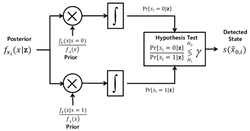
In order to perform the hypothesis test in (5), the decoder needs to calculate a probability ratio $\frac{{\Pr\{s_{i}=0|{\bf{z}}\}}}{{\Pr\{s_{i}=1|{\bf{z}}\}}}$. By factorizing over $x_{i}$, the ratio becomes

$${\frac{{\Pr\{s_{i}=0|{\bf{z}}\}}}{{\Pr\{s_{i}=1|{\bf{z}}\}}}}={\frac{{\int{\Pr\{s_{i}=0|{\bf{z}},x_{i}\}f_{x_{i}}(x|\mathbf{z})}dx}}{{\int{\Pr\{s_{i}=1|{\bf{z}},x_{i}\}f_{x_{i}}(x|\mathbf{z})}dx}}}\mathop{\mathop{\gtrless}\limits_{{H_{1}}}}\limits^{{H_{0}}}1,$$ (9)

where $f_{x_{i}}(x|\mathbf{z})$ denotes the posterior density of $x_{i}$ given $\mathbf{z}$. In (9), $\Pr\{s_{i}|{\bf{z}},x_{i}\}=\Pr\{s_{i}|x_{i}\}$ holds true since the measurements $\mathbf{z}$ do not provide any additional information on $s_{i}$ given $x_{i}$. Using the Bayesian rule and the prior information, the test in (9) is rewritten as

$${\frac{{\int{\frac{{f_{x}(x|s=0)}}{{f_{x}(x)}}f_{x_{i}}(x|\mathbf{z})}dx}}{{\int{\frac{{f_{x}(x|s=1)}}{{f_{x}(x)}}f_{x_{i}}(x|\mathbf{z})}dx}}}\mathop{\mathop{\gtrless}\limits_{{H_{1}}}}\limits^{{H_{0}}}{\frac{{\Pr\{s=1\}}}{{\Pr\{s=0\}}}}=\gamma,$$ (10)

where $\gamma:={\frac{q}{(1-q)}}$. Therefore, the probability ratio is obtained from the corresponding posterior and prior densities. The overall flow of the hypothesis test for a supportive state detection is shown in Fig.1.

Figure 1: Bayesian hypothesis test for a state detection

III-C Belief Propagation for Posterior Approximation

The posterior density $f_{x_{i}}(x|\mathbf{z})$ used in the hypothesis test is obtained by BP. Using Bayesian rule, we can represent the posterior density $f_{x_{i}}(x|\mathbf{z})$ in the form of ${\rm{Posterior=Prior}}\times\frac{{{\rm{Likelihood}}}}{{{\rm{Evidence}}}}$, given as

$$f_{x_{i}}(x|\mathbf{z})=f_{x}(x)\times\frac{{f_{\mathbf{z}}({{\bf{z}}|x_{i})}}}{f_{\mathbf{z}}(\mathbf{z})}.$$ (11)

If the measurement matrix $\mathbf{\Phi}$ is sufficiently sparse such that the corresponding bipartite graph is tree-like, we postulate that the elements of $\mathbf{z}$ associated with $x_{i}$ are independent each other [10]. Under the tree-like assumption, we can decompose the likelihood density $f_{\mathbf{z}}({\bf{z}}|x_{i})$ to the product of densities:

$$f_{x_{i}}(x|\mathbf{z})\propto f_{x}(x)\times\prod\limits_{j:\phi_{ji}\neq 0}f_{z_{j}}({z}|{x_{i}}).$$ (12)

Since each element of $\mathbf{z}$ is represented by the sum of independent random variables with $\mathbf{\Phi}$, we can expressed $f_{z_{j}}(z|x_{i})$ as linear convolution of associated density functions, given as

$$\begin{array}[]{l}f_{z_{j}}(z|x_{i})=\\ \delta(z-z_{j})\otimes f_{n_{j}}(n)\otimes\left(\bigotimes\limits_{k:\phi_{jk}\neq 0,k\neq i}{f_{x_{k}}}(x)\right).\end{array}$$ (15)

The essence of the BP-process is to obtain an approximation of $f_{x_{i}}(x|\mathbf{z})$ from iterative mutual update of probability messages. The message update rule is formulated based on (12),(15). We follow the rule introduced in [15], given as

$$\mathbf{a}_{i\rightarrow j}^{l}:=\eta\left[{{f_{x}}(x)\times\prod\limits_{k:\phi_{ki}\neq 0,k\neq j}{{\bf{b}}_{k\rightarrow i}^{l-1}}}\right],$$ (16)

$$\mathbf{b}_{j\rightarrow i}^{l}:=\left({\mathop{\bigotimes}\limits_{k:\phi_{jk}\neq 0,k\neq i}{\bf{a}}_{k\to j}^{l}}\right)\otimes\delta(z-z_{j})\otimes f_{n_{j}}(n),$$ (17)

$\text{ for all }(i,j)\in\{1,...,N\}\times\{1,...,M\}:|\phi_{ji}|=1$, where $\otimes$ and $\bigotimes$ are the operator for linear convolution and the linear convolution of a sequence of functions, respectively; $\eta(\cdot)$ denote a normalization function for probability densities;, and $l$ denotes the iteration index. The probability messages $\mathbf{a}_{i\rightarrow j}$ and $\mathbf{b}_{j\rightarrow i}$ are mutually updated via BP-iterations. Then, we approximate the posterior density $f_{x_{i}}(x|\mathbf{z})$ after a certain number of iterations $l^{*}$ as follows:

$$f_{x_{i}}(x|\mathbf{z})\approx\eta\left[{f_{x}(x)\times\prod\limits_{j:\phi_{ji}\neq 0}{{\mathbf{b}_{j\rightarrow i}^{l^{*}}}}}\right].$$ (18)

IV Numerical Results

We demonstrate the performance of BHT-BP via simulation results. We consider the SER performance given in (6) and take 1000 Monte Carlo trials for each experimental point to show the average performance. In each trial, we generate a deterministic sparse vector $\mathbf{x}_{0}$ with $N=128$. The generation of $x_{i}$ belonging to the support set follows zero mean Gaussian distribution with $\sigma_{x}=10$; but we restrict the magnitude level to $\sigma_{x}/5\leq|x_{i}|\leq 3\sigma_{x}$. For the measurement matrix $\mathbf{\Phi}$, BHT-BP uses sparse-Bernoulli matrix with $L=3$.

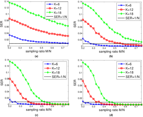
Fig.2 shows the SER performance as a function of undersampling ratio $M/N$ for a variety of SNR and $K$. Naturally, BHT-BP is well performed as SNR increases. However, BHT-BP works similarly beyond 30 dB as shown in Fig.2-(c),(d). Regarding the signal sparsity $K$, BHT-BP needs at least SNR $\geq 30$ dB to recover the support with SER below the $1/N\approx 0.0078$ for $K\leq 18$ if $M/N$ is sufficient.

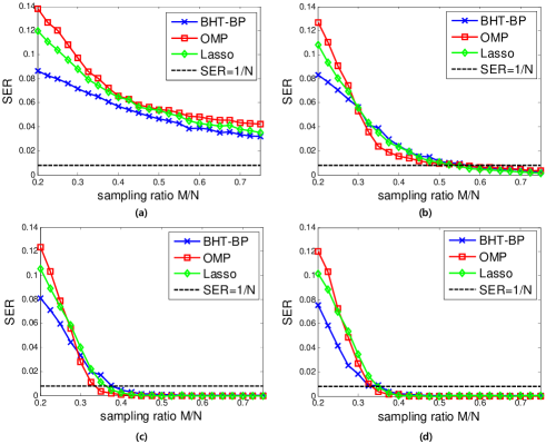
Fig.3 shows the advantages of BHT-BP compared to OMP [17] and Lasso [18]. The source codes of OMP and Lasso were obtained from SparseLab 2.0 package (available at http://sparselab.stanford.edu/). OMP and Lasso use a Gaussian measurement matrix having the same column energy as the sparse-Bernoulli matrix for fairness, i.e., $\left\|{\mathbf{\phi}_{j,Gaussian}}\right\|_{2}^{2}=\left\|{\mathbf{\phi}_{j,Sparse}}\right\|_{2}^{2}=L$. In addition, we choose the $K$-largest values from $\widehat{\mathbf{x}}_{0}$ for the support detection of OMP and Lasso. We generate $\mathbf{x}_{0}$ with $N=128$ and $K=12$ in this simulation. At SNR=10 dB, we can see that BHT-BP outperforms Lasso and OMP as shown in Fig.3-(a), because the use of noise statistic $f_{n_{j}}(n)$ in the BP-process provides the precise posterior information, and it leads to reducing of misdetection of the supportive state $\widehat{s}_{0,i}$ in the hypothesis test. Nevertheless, the SER curves at SNR=10 dB are far from $SER=1/N$ due to the noise effect. Such a fact is supported by the theoretical work in [6] where the ML decoder needs $M/N\geq 1.02$ for exact support recovery when SNR=10 dB.

As SNR increases, all algorithms are gradually performed similarly, but Lasso and OMP have slightly lower cross point to SER$=1/N$ as shown in Fig.3-(b),(c),(d) and Table I. Such a result is caused by sensing inefficiency from the use of sparse measurement matrices [8]. However, BHT-BP has advantage on low computational cost and the fast measurement generation with the sparse matrix. Indeed, BHT-BP has the lower cost $O(N\log N)$ by aid of BP, than OMP $O(KNM)$ and Lasso $O(NM^{2})$.

Figure 2: SER performance of BHT-BP over $M/N$ for a variety of SNR and $K$: (a) SNR=10 dB, (b) SNR=20 dB, (c) SNR=30 dB, (d) SNR=50 dB.

Figure 3: SER performance comparison to OMP and Lasso over $M/N$ when $K=12$: (a) SNR=10 dB, (b) SNR=20 dB, (c) SNR=30 dB, (d) SNR=50 dB.

TABLE I: Cross point in $M/N$ to SER$=1/N$ when $K=12$

Algorithms / SNR	50 dB	30 dB	20 dB	10 dB
BHT-BP	0.357	0.375	0.575	-
Lasso	0.350	0.361	0.550	-
OMP	0.331	0.335	0.552	-
ML limit for exact	0.101	0.1108	0.1935	1.021
recovery in [6]

V Summary

We proposed a new support recovery algorithm using belief propagation called BHT-BP. Our proposed algorithm utilizes hypothesis test to detects the support set from noisy measurements where posterior used in the test is provided by belief propagation. Our numerical results showed that the proposed algorithm outperforms OMP and Lasso in the low SNR regime, and becomes working similarly as SNR increases. However, the proposed algorithm still has strength in terms of low computational cost and the fast measurement generation by the use of the sparse matrix and belief propagation.

VI Acknowledgment

This work was supported by the National Research Foundation of Korea (NRF) grant funded by the Korea government(MEST) (Haek-Sim Research Program, NO. 2011-0027682, Do-Yak Research Program, NO. 2012-0005656)

References

- [1] D.L. Donoho, “Compressed sensing,” IEEE Trans. On Information Theory, vol. 52, pp. 1289-1306, 2006.
- [2] A. J. Miller, Subset Selection in Regression. New York: Chapman & Hall, 1990.
- [3] R. A. DeVore and G. G. Lorentz, Constructive Approximation. New York: Springer-Verlag, 1993.
- [4] M. J. Wainwright, “Sharp thresholds for noisy and high-dimensional recovery of sparsity using -constrained quadratic programming (lasso),” IEEE Trans. Inf. Theory, vol. 55, no. 5, pp. 2183-2202, May 2009.
- [5] A. K. Fletcher and S. Rangan, “Orthogonal matching pursuit from noisy random measurements: A new analysis,” in Proc. conf. Neural Information Processing Systems, Vancouver, BC, Canada, Dec. 2009.
- [6] A. Fletcher, S. Rangan, and V. Goyal, “Necessary and sufficient conditions for sparsity pattern recovery,” IEEE Trans. Inform. Theory, vol. 55, no. 12, pp. 5758-5772, Dec. 2009.
- [7] K. R. Rad, “Nearly sharp sufficient conditions on exact sparsity pattern recovery,” IEEE Trans. Inf. Theory, vol. 57, no. 7, pp. 4672-4679, May 2011.
- [8] W. Wang, M. Wainwright, and K. Ramchandran, “Information-theoretic limits on sparse signal recovery: Dense versus sparse measurement matrices,” IEEE Trans. Inf. Theory, vol. 56, no. 6, pp. 2967-2979, Jun. 2010.
- [9] M. Akcakaya and V.Tarokh, ”Shannon-theoretic limit on noisy compressive sampling,” IEEE Trans. Inf. Theory, vol. 56, no. 1, pp. 492-504, Jan. 2010.
- [10] T. Richardson, and R. Urbanke, “The capacity of low-density parity check codes under message-passing decoding,” IEEE Trans. Inform. Theory, vol. 47, no. 2, pp. 599-618, Feb. 2001.
- [11] R.G. Gallager, Low-Density Parity Check Codes, MIT Press: Cambridge, MA, 1963
- [12] D. Baron, S. Sarvotham, and R. Baraniuk, “Bayesian compressive sensing via belief propagation,” IEEE Trans. Signal Process., vol. 58, no. 1, pp. 269-280, Jan. 2010.
- [13] X.Tan and J. Li, “Computationally efficient sparse Bayesian learning via belief propagation,” IEEE Trans. Signal Process., vol. 58, no. 4, pp. 2010-2021, Apr. 2010.
- [14] M. Akcakaya, J. Park, and V. Tarokh, “A coding theory approach to noisy compressive sensing using low density frame,” IEEE Trans. Signal Process., vol. 59, no. 12, pp. 5369-5379, Nov. 2011.
- [15] J. Kang, H.-N. Lee, K. Kim, “On detection-directed estimation approach for noisy compressive sensing,” 2011 [Online]. Available:arXiv:1201.3915v3 [cs.IT].
- [16] H. Ishwaran and J. S. Rao, “Spike and slab variable selection : Frequentist and Bayesian strategies,” Ann. Statist., vol.33, pp. 730-773, 2005.
- [17] J. A. Tropp and A. C. Gilbert, “Signal recovery from random measurements via orthogonal matching pursuit,” IEEE Trans. Inf. Theory, vol. 53, no. 12, pp. 4655.4666, Dec. 2007.
- [18] R. Tibshirani, “Regression shrinkage and selection via the lasso,” J. Roy. Statisti. Soc., Ser. B, vol. 58, no. 1, pp. 267.288, 1996.