Connections between the Sznajd Model with General Confidence Rules and graph theory
Abstract
The Sznajd model is a sociophysics model, that is used to model opinion propagation and consensus formation in societies. Its main feature is that its rules favour bigger groups of agreeing people. In a previous work, we generalized the bounded confidence rule in order to model biases and prejudices in discrete opinion models. In that work, we applied this modification to the Sznajd model and presented some preliminary results. The present work extends what we did in that paper. We present results linking many of the properties of the mean-field fixed points, with only a few qualitative aspects of the confidence rule (the biases and prejudices modelled), finding an interesting connection with graph theory problems. More precisely, we link the existence of fixed points with the notion of strongly connected graphs and the stability of fixed points with the problem of finding the maximal independent sets of a graph. We present some graph theory concepts, together with examples, and comparisons between the mean-field and simulations in Barabási-Albert networks, followed by the main mathematical ideas and appendices with the rigorous proofs of our claims. We also show that there is no qualitative difference in the mean-field results if we require that a group of size , instead of a pair, of agreeing agents be formed before they attempt to convince other sites (for the mean-field, this would coincide with the -voter model).
pacs:
02.50.Ey, 02.60.Cb, 05.45.Tp, 05.65.+b, 89.65.-sI Introduction
In the last years, the interest in interdisciplinary problems has increased among physicists, creating many research areas. One of these areas is sociophysics, that studies how assumptions about the behaviour and social interactions of people in a “microcospic level” creates emerging social behaviours, like opinion propagation, consensus formation, properties of elections, how wealth is distributed in society, among other topics. Typical approaches include modelling using deterministic celular automata, Monte Carlo simulations of models derived from ferromagnetic models (usualy Ising and Potts), mean-field approaches and diffusion-reaction processes votante-def ; sznajd-def ; deffuant-def ; HK-def ; ochrombel-def ; axelrod-def ; Galam-2004 ; Castellano-2009 .
The Sznajd model is an opinion propagation model, originally inspired by the Ising model in a linear chain, and is typically used to model consensus formation. It has spawned many variations, including the addition of noise, contrarian-like agents and undecided voters; as well as generalizations to more than 2 states (opinions) and to arbitrary networks sznajd-def ; Bernardes-2002 . In all these variations, the most defining aspect of the Sznajd model is that it gives a greater convincing power to bigger groups of agreeing agents. Even though the importance of this effect has been known by psychologists since the 1950s Asch-1951 , it is often overlooked in other opinion propagation models, for the sake of simplicity (this happens for example in the voter and in the Deffuant models votante-def ; deffuant-def ).
In a recent work, we took the bounded confidence rule (that roughly says that people are only allowed to change opinions in a smooth way) that is common to many opinion propagation models deffuant-def ; HK-def ; Stauffer-2001 , including the Sznajd model, and we generalized it to model biases and prejudices in discrete opinion models (these generalized rules will be called by the umbrella term confidence rules). We applied this generalization to the Sznajd model and studied mainly the case with 3 opinions. In that work, we found a good qualitative (and in some cases quantitative) agreement between the model simulated in Barabási-Albert (BA) networks rede-BA-def and the mean-field equations, but some of the results about the mean-field were still rather sketchy. In the present paper we give rigorous proofs (the main mathematical ideas are in a sepparate section and the detailed proofs can be found in the appendices) about the structure, existence and stability of the fixed points for the mean-field version of the Sznajd model with general confidence rules, finding a connection between these properties and graph theory problems using a graph derived only from qualitative properties of the confidence rule.
The results have some counterintuitive aspects and as such we provide both numerical solutions for the mean-field equations and Monte Carlo simulations for the model in a BA network. In our calculations for the mean-field, we use a variant of the model, where at each timestep we choose agents and if they agree, they attempt to convince other agents; and show that there is no qualitative difference between all the cases with (which includes the usual definition of the Sznajd model in an arbitrary network, with an arbitrary number of opinions, as we have considered in Timpanaro-2009 ).
II The Sznajd model with confidence rules
The Sznajd model is an agent based sociophysics model for opinion propagation. In this model, a society is represented by a network (that is, a collection of nodes linked together by edges), where each node represents an agent (person), each edge is a social connection (friendship, marriage, acquaintances, etc.) and each node possesses an integer , between 1 and , representing its opinion. In our generalization of the Sznajd model, as defined in Timpanaro-2009 , we introduce a set of parameters (that are fixed and completely independent with the state of the network), and at each time step the following update rule is used:
-
•
A node is chosen at random, and then a neighbour of is chosen.
-
•
If they disagree (), nothing happens.
-
•
If they agree, a neighbour of is chosen and is convinced of opinion with probability .
We can interpret the first step as a conversation between two people that know each other, where they discuss some issue. If they disagree, none manages to convince the other. But, if they agree, they may set to convince another person that one of them knows and this person is convinced with a certain probability that depends only of its current point of view and of the opinion the pair is trying to impose.
In the original model the probability weights are not dependent on and . The reason why this probability should depend on both opinions is that, usualy an opinion includes prejudices about differing points of view (this is strongly related with the idea of cognitive dissonance in psychology Festinger-cog-dis ; Elster-cog-dis ; Lee-cog-dis ). This generalization allows for complex interactions among the opinions in an unified way and can be seen as a generalization of the bounded confidence rules deffuant-def ; HK-def , as those rules can be recovered as special cases. Other modifications of the model can also be obtained this way:
-
•
When we have the usual model.
-
•
If and otherwise, we have bounded confidence with threshold .
-
•
Undecided agents can be modelled by a special state , such that (undecided agents can only be convinced).
-
•
Cyclic interactions, like rock, paper, scissors ( convinces only , that convinces only , that convinces only ).
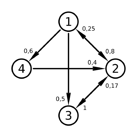
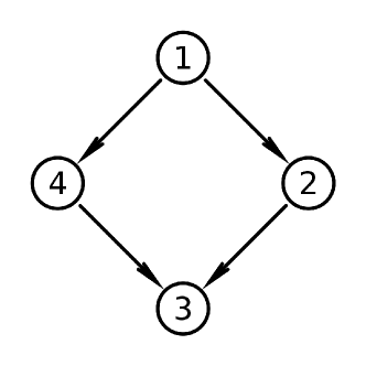
This generalized version of the model has parameters, where is the number of opinions ( is irrelevant and can always be taken as 0). These parameters can be thought as the elements of the adjacency matrix of a directed weighted graph, that will be refered to as confidence rule (we will also refer to the parameters in this way). So the confidence rule is a directed weighted graph, whose nodes are the opinions in the model (so a model with opinions would have a confidence rule with nodes) and the arcs represent the ways that opinions are allowed to interact. This graph is useful as a way of schematizing the opinion interactions and as we show in the next sections, it can be used to find the properties of the mean-field fixed points. An example of confidence rule with 4 opinions is given in figure 1.
II.1 The mean-field model
For the analysis of the mean field case, we consider a variant of the Sznajd model, where at each timestep we choose agents at random and if they agree (meaning they are on the same state), they attempt to convince other agents (also chosen at random). If the group of agents has opinion , then each of the targeted agents is convinced with probability and retains its opinion with probability , where is the opinion the targeted agent had before the group attempted to convince it (and hence it is different for each of the agents). Adding up the probabilities of all possible processes we obtain the mean field equation in the limit of large networks:
| (1) |
where is the proportion of sites with opinion (the deduction of this equation from the underlying Markov chain implies that is actually the expected value of the proportion) and a time unit corresponds to a Montecarlo timestep (MCT), that is, a number of timesteps equal to the number of sites in the network. The phase space of this flow is an -simplex denoted as (that is embedded in an dimensional vector space, in order to make the equations more symmetrical), where the vertices correspond to consensus states and the other states are convex combinations of the vertices, with coeficients :
| (2) |
where is the coordinate of the vertex corresponding to consensus of opinion and is the coordinate in phase space of the point representing the state (in other words, we’re using a barycentric coordinate system).
The results for the mean-field fixed points can be expressed as problems regarding the existence of groups of nodes satisfying certain conditions in the confidence rule and these results are the same for all . We will give here these results for a better understanding of the simulations in section III, leaving the mathematical details for later. Because of the connection of these results with graph theory, a small glossary (with examples) will be useful. For the same reason, we will interchange freely the notion of a set of opinions with the notion of a set of nodes in some graph (like the confidence rule).
II.2 Graph theory concepts and glossary
If is a weighted graph, with adjacency matrix (that is, the matrix containing the weights of the graph) and , one can define its directed skeleton as the directed graph with adjacency matrix:
An example of skeleton is given in figure 2.
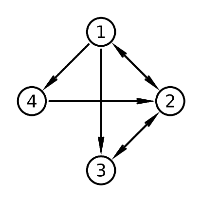
Let now be a set of nodes in a directed graph (typically in our problems, will be a set of opinions and will be the skeleton of the confidence rule). We define the following terms (we will use in the examples equal to the graph in figure 2):
-
•
The predecessor set of , denoted by , is the set of nodes in that point to some node in . For example, and .
-
•
Analogously, the successor of , denoted by , is the set of nodes in that are pointed by nodes in . For example, .
-
•
The complement of , is the set of nodes in that are not in . For example, .
-
•
is an independent set iff has no connections among nodes in . and are independent sets. Note that if is independent, it follows that .
-
•
An independent set is maximal if it contains all the nodes in the graph or if the addition of any node not in destroys independence. is a maximal independent set, while is independent but not maximal.
-
•
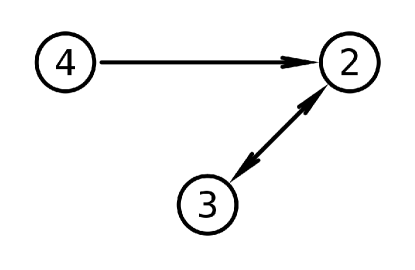
If is a set of nodes from , then the graph induced by , is the graph whose set of nodes is and whose connections are the connections between the elements of that existed in . The graph can be found in figure 3.
-
•
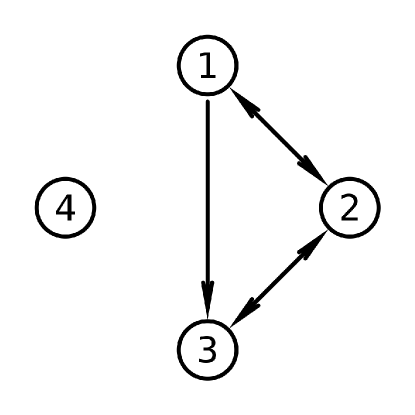
The union of 2 graphs and , denoted is the graph with all the nodes of and , but only connections that already existed between and (in short it means referring to 2 unrelated graphs as parts of the same graph, without changing anything else). The graph is shown in figure 4. Also, the more familiar concept of component can be defined as a graph that is not the union of any smaller parts and is also not part of a larger graph with the same property.
-
•
A graph is strongly connected if we can start at any node and get to any other node, respecting the directions of the arcs. , and are strongly connected, but is not because there is no path from 3 to 1 in it.
Finaly, we will denote by the manifold with the states where only opinions in survive:
| (3) |
II.3 Mean-field results
Let be the skeleton of the confidence rule. The results for the mean-field fixed points are:
-
•
Given a fixed point, its stability properties depend only on which opinions survive in it and on the skeleton of the confidence rule.
-
•
There exists a fixed point, where all opinions survive, iff is a union of strongly connected graphs. Moreover, if itself is strongly connected, this point is unique and an unstable node (the only exception is the case with 1 opinion, when the fixed point is the only point in the phase space). This is equivalent to the more intuitive statement that there exists a fixed point where all opinions coexist iff we cannot build a set of opinions that can convince opinions in , but cannot be convinced by any opinion in .
-
•
The results concerning only opinions in a set (the fixed points and the stabilities inside ) can be found using the model defined by the confidence rule . (in other words, removing opinions from the model leaves us with a model with a different confidence rule, that is valid inside of ).
-
•
If can be split in 2 independent models, that is, . Then for all and , fixed points of the models with rules and respectively, all the points with are fixed points of the model with rule . Moreover, the number of unstable directions and stable directions is the respective sum of the numbers for and (when considering only directions inside and ). The same thing is true for the neutral directions along which there is movement, but fails for the ones with no movement (we must add as an extra direction in this case).
-
•
A fixed point where only opinions in survive is attractive iff . This also implies that is a maximal independent set (see appendix A.1) and hence that is an attractor.
These results have some interesting consequences and interpretations, that should be kept in mind when analysing the simulation results.
-
•
The mean-field has no stable situations where 2 interacting opinions coexist. This means that all possible (static) attractors are of the form , where is a maximal independent set.
-
•
The requirement that be maximal for to be an attractor allows the existence of attractors with surviving opinions that do not convince any opinions at all.
-
•
The condition implies that it is possible to build confidence rules that have no such attractors. These rules display heteroclinic cycles (see appendix A.2), which cause oscilations with diverging period and are heavily affected by finite size effects during simulations.
-
•
If every opinion can convince any other (that is for all ), then the consensus states are the only attractors.
-
•
In situations where part of the confidence rule can be broken in different components, by the removal of some opinions, there are manifolds where all points are fixed points, and these manifolds can be analised by putting together the analysis of each of the components.
III Simulation Results and Examples
For our simulations, we used Barabási-Albert networks with sites and minimal connectivity equal to 5 (we used different networks, but always with these same parameters).
In order to compare trajectories obtained by simulations with trajectories obtained by integrating equations (1) we recall that is the expected value of the proportion of sites with opinion . Because of this and in order to reduce noise, we take averages over many simulations (one can also reduce noise by choosing a larger network size). More importantly, if the initial condition for the mean-field equations is , then this means that for the corresponding simulations, each site must have its opinion chosen at random with probability for opinion .
The simulations we will do will be aimed at giving examples of the mean-field results from section II.1, some of their counter-intuitive aspects and some divergences between the simulations and the mean-field.
III.1 Attractors and stability
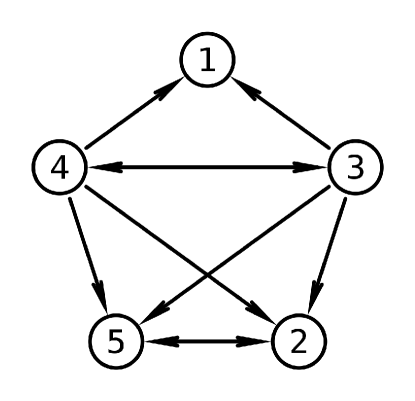
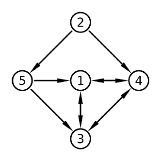
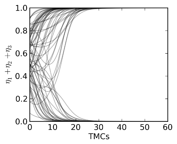
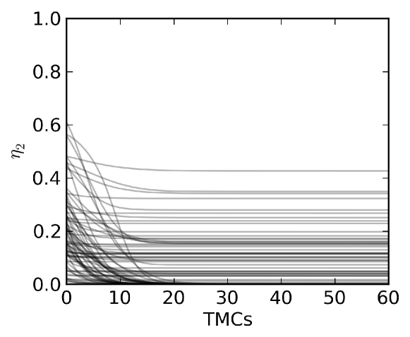
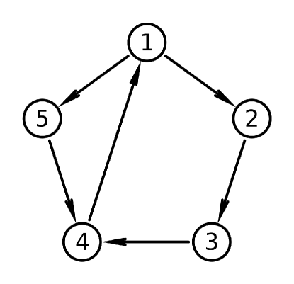
To illustrate the results about the stability properties of the fixed points, consider the rule , depicted in figure 5 (actualy, a family of confidence rules). The maximal independent sets are and , but only and obey , meaning that the only stationary attractors are and . After a transient we see one of 2 situations, the only surviving opinions will be 1 and 2 or they will be 1 and 5. We can see this from the time series of (it tends to 1) and (it tends to 0, although with a longer transient) (figures 6(a) and 6(b)).
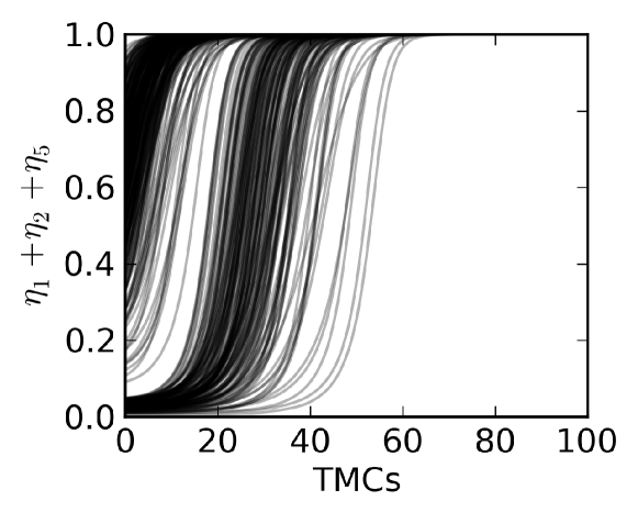
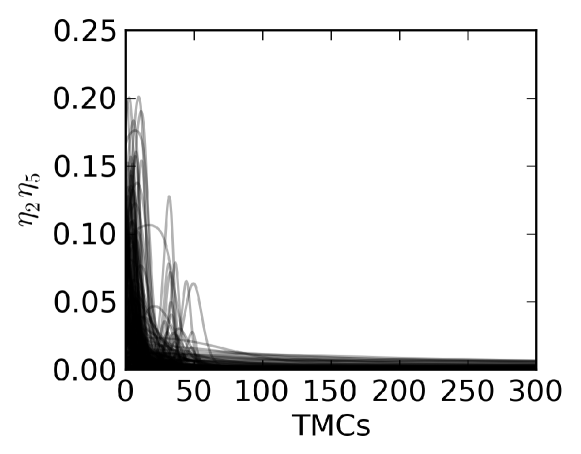
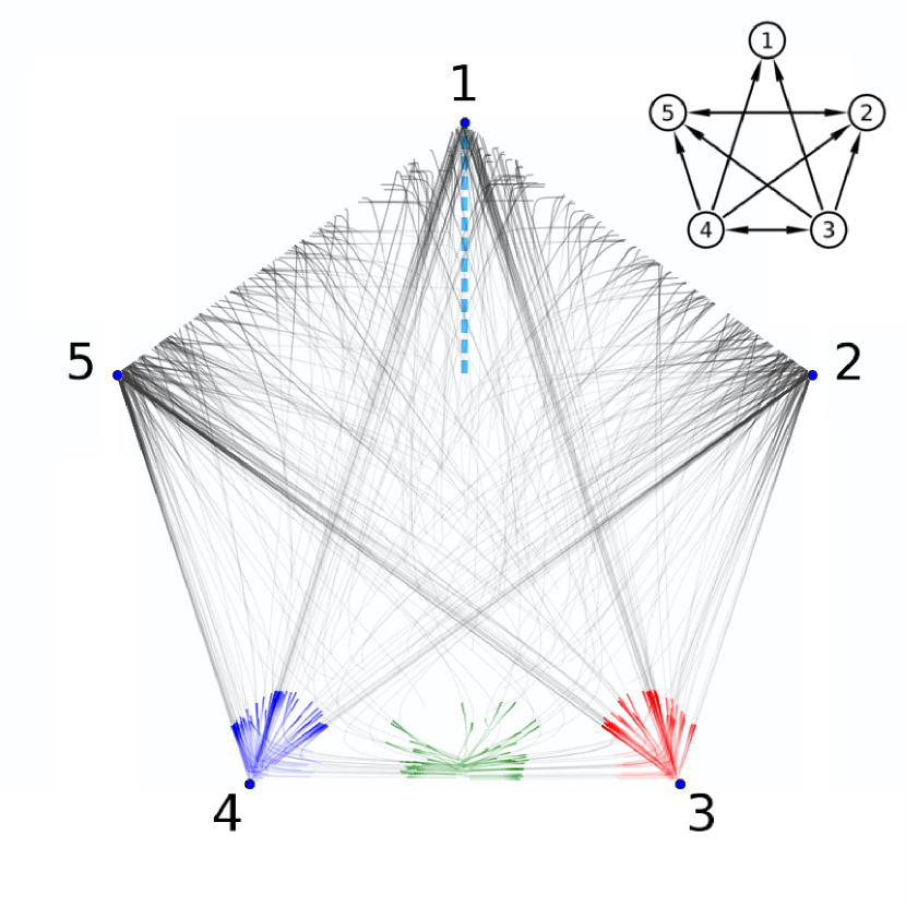
The other fixed points can be found by looking at the other induced graphs that are unions of strongly connected graphs. They are , , and . Note that and that both components are strongly connected. This means that we will actualy have a line of fixed points connecting some point in the edge to the vertex . The stability properties of these points are in table 1. A projection of the phase space (where the weights in the confidence rule where taken as 0 or 1), showing the attractors and the features described in this table can be found in figure 7.
| 3 | 1,2,4,5 | 4 | 1,2,4,5 | 3 | 1 | 0 |
| 4 | 1,2,3,5 | 3 | 1,2,3,5 | 3 | 1 | 0 |
| 3,4 | 1,2,5 | 3,4 | 1,2,3,4,5 | 4 | 0 | 0 |
| ,5 | 3,4 | 2,3,4,5 | 2,5 | 1 | 2 | 1 |
III.2 Surviving inert opinions
Next, we consider two examples in which we have opinions that survive in an attractor, but don’t convince any other opinion (we’ll call them inert). Consider the rules and given in figure 8. In , is an attractor, even though opinion 1 is inert (can’t convince any of the others). In , , and are attractors, even though opinion 2 is inert.
We now check that this effect is present in the simulations. Time series for the models with confidence rules and (once again, the weights are taken as 0 or 1) are given in figures 9(a) to 9(d).
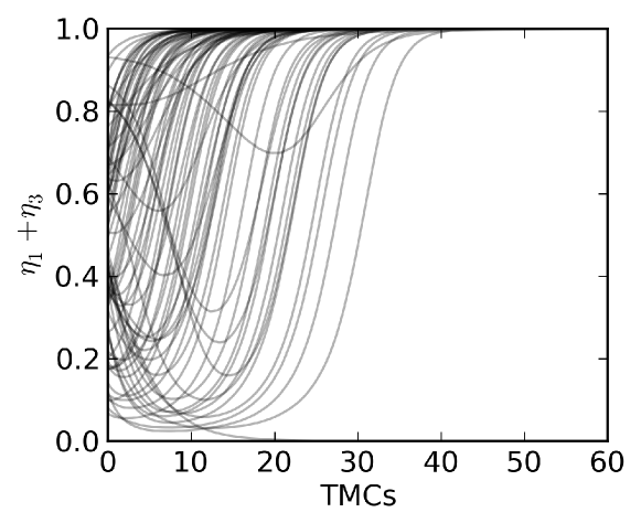
Time series for the rules and .
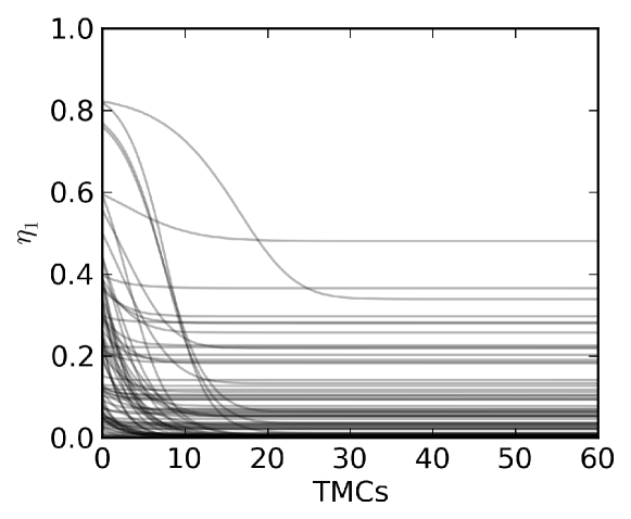
*(cont.)
*(cont.)
III.3 Rules without stationary attractors
Consider a rule in which all opinions interact (that is, for all pair of distinct opinions and either or ), but such that every opinion has at least one different opinion that it can’t convince. The independent sets of such rule are all unitary, but we have imposed that and , so there are no solutions to for this rule and hence it has no stationary attractors (it is possible to build other types of examples as well). An example for 4 opinions is given in figure 9.
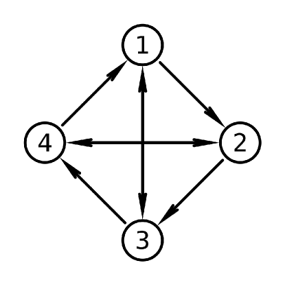
In the appendix A.2 we prove that if a graph has no solutions to , then it has at least one directed cycle, where no edge is doubly connected. In the phase space, these cycles manifest themselves as heteroclinic cycles. These cycles will always be polygonal curves connecting the vertices of the simplex that correspond to the nodes the cycle in the graph goes through. Moreover, as the cycle goes through the nodes in , it means that induces in the confidence rule a strongly connected graph with one component and as such, there exists an unstable fixed point where all the opinions in coexist (in the example of figure 9 the cycle would be , corresponding to the heteroclinic cycle and to an unstable fixed point where all opinions coexist). Hence, the heteroclinic cycle is fully contained in the border of and there is a fixed point in the bulk of that leads the trajectories to its border. The typical result is that as time goes by, the trajectories get closer to one of the cycles, which causes oscillations with a diverging period (as they pass each time closer to the consensus states, that are fixed points). In simulations, eventually a random fluctuation puts the system in a state where one of the opinions in the cycle gets extinct, leading the system to a stationary state.
III.4 Long transients and stationary states
In many simulations, there are situations in which the trajectories get stuck for long times in states that are not attractors. In some of these cases, the simulation got to a stationary state where there are no active connections between the agents (that is, a connection between a pair of agreeing sites and a neighbour that they can convince, according to the confidence rule). In other cases there are active connections, but some opinions appear in negligible amounts and the set of opinions that are not negligible forms an independent set, but not a solution to . In the latter cases, the fixed points in are saddle points meaning that (this is shown in detail in section IV.1) and usually, one (or more) of the negligible opinions will be able to rise again, causing long transients.
Considering the mean-field equations, if (meaning that is negligible), then it evolves according to (see section IV.1 for further explanations)
| (4) |
as long as the opinions in are negligible. This implies that the time the trajectories spend close to these saddle points can be estimated, considering the time it takes for some of the opinions in to duplicate its proportion of sites in the network (all the other opinions in will remain negligible for much longer times, see appendix D). Solving 4 we get
| (5) |
We now verify this relation for the integration of the mean-field equations and compare these results with the simulations. We will use the rule in figure 10, with .
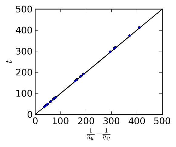
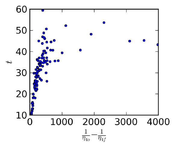
For this choice of confidence rule and opinion set, we can approximate equation 4 with
| (6) |
IV Analytical Results
IV.1 Stability and structure of the fixed points
This equation is a flow where the phase space is the simplex defined by
and it is easy to show that all trajectories starting in the simplex never leave it (the sum is 0 because the term being summed in equation 1 is skew-symmetrical and the sign of the variables doesn’t change because is bounded in the bulk of the phase space).
Let us define , and , implying that . Let us also denote the skeleton of the confidence rule by . The fixed points of equation 1 are given by
| (7) |
for each opinion . If is a fixed point (meaning, the represented point in phase space is a fixed point), then one can look at the behaviour of trajectories close to it, using the spectrum of the jacobian of , evaluated at . The jacobian of , is given by
| (8) |
For each fixed point , we can define two sets of opinions, and , respectively the set of opinions that survive and that are extinct in . It is also useful to look at the components induced by : . That is,
The jacobian , can be simplified when it is evaluated at the fixed point and (we will denote all quantities evaluated at the fixed point by adding a superscript):
| (9) |
implying that the jacobian can be written up to permutations as
| (10) |
where is the jacobian restricted to the opinions in and is the one restricted to (that is a diagonal matrix). It also follows from equation 8 that can be written in a block-diagonal form where each block is the jacobian restricted to the component :
| (11) |
so in order to find the spectrum of , we need to put together the spectrum of (which is trivial to find) with the spectrum of each of the blocks . This means that all that is left is to find the spectrum of the jacobian in a coexistence fixed point, for a rule with one component. We show in the appendix C that, if , all the eigenvalues of have positive real part in this situation and the corresponding eigenvectors are parallel to the phase space, with the exception of one eigenvector that is not parallel and has eigenvalue 0 (with multiplicity 1). As this last eigenvector doesn’t take points in the phase space to other points in the phase space it is irrelevant to the stability analysis. This null eigenvalue can be regarded as an artifact of having embedded an -dimensional phase space in dimensions. However, according to our reasoning based in equation 11, it does mean that if induces components, there are eigenvalues equal to 0. To understand what these null eigenvalues mean, consider the case . We define and as the vectors containing only the coordinates of and that are in , that is
We also define the vectors as
For every , is a function of only . Moreover, is homogeneous with order , so if
| (12) |
It follows that all the points given by
| (13) |
are fixed points of the model. The set of points defined by equation 13 is the convex hull of the points defined by the (we identify these vectors with points in the phase space using equation 2) and as these vectors are linearly independent, it means the convex hull must have dimensions.
Euler’s theorem gives us another consequence of the homogeneity of , namely
| (14) |
So in the fixed point we have , yielding a base of eigenvectors with eigenvalue 0. These eigenvectors can be reorganized so that they are still linearly independent, but only one of them points outwards from the phase space, meaning that said eigenvector is irrelevant to the stability analysis (the embedding artifact previously discussed). Such a base can be taken as , , together with . Removing the artifact, we have a base that generates the flat defined by equation 13. As all the points in the flat are fixed points, this means that there is no movement along these directions for trajectories close to the fixed points.
Finaly, we need to study the spectrum of . As this is a diagonal matrix, we can obtain the eigenvalues directly:
| (15) |
for each and the eigenvalue tells us if the trajectories are attracted or repelled to the manifold .
It follows that if is such that , then for all and we have a complete picture of the behaviour of trajectories close to the fixed point. On the other hand, if , some of these eigenvalues are null and we need to examine higher orders. In order to do that, if , then we must make a Taylor expansion of around . As is given by
then it is easy to see that the lower order term, different from 0 yields
| (16) |
meaning that the trajectories are repelled from the manifold , unless . In particular, for and , the solution of equation 16 reads
Let be the manifold where only opinions in survive. We then know that if all , the trajectories get attracted to , but if and for any , then the trajectories get repelled from . Finaly, suppose that either or for all opinions in . Let be the set of opinions such that ,
We show in the appendix D that starting in a sufficiently close neighbourhood of the following inequality holds
| (17) |
and so trajectories are neither attracted to nor repelled from .
We can now put all these results together. If is a fixed point, such that has components, then the trajectories in a neighbourhood of are such that (remembering that ):
-
•
There are unstable directions.
-
•
There are stable directions.
-
•
There are directions along which there is no movement.
-
•
There are directions that are neither attractive nor repulsive, but along which there is movement.
It follows from the equations 1 that if is independent, then is composed entirely of fixed points. On the other hand, if is attractive, then it has no unstable directions and the only neutral directions are those along which there is no movement, so if is the number of components of , then and it follows that
| (18) |
implies that is independent. The condition that there are no neutral directions yields
| (19) |
This implies that
As is independent, and so , implying
As is independent we have . So, as always solves equations 18, it follows that is attractive iff is independent and . As we show in appendix A.1, alone implies that is maximal independent, so to find the attractors of the model it suffices to find all the sets , satisfying and the corresponding manifolds .
IV.2 Existence of the fixed points
In the last section, we analysed the stability properties of a fixed point, supposing that it existed (given a fixed point, what its stability properties are). Now we check when a fixed point, where only the opinions in a given set coexist, exists. Our analysis of the case in which the set of surviving opinions induces more than one component in the confidence rule shows us that we only need to study the case in which all the opinions coexist and the confidence rule has one component.
In this case, any fixed point where all opinions coexist must be an unstable node, if it exists, and so if we had embedded our phase space in instead of dimensions (substituting by , for example), the jacobian of the corresponding flux would be a real matrix that is positive definite when evaluated in such a fixed point, implying that . It follows that the index of the fixed point is 1 111The index in the case when the jacobian is not singular equals the sign of its determinant. More information about indices and their meaning can be found in most textbooks about differential geometry. and that we can apply the implicit function theorem in this case.
In the appendix E, we use these informations together with the Poincaré-Hopf theorem to show that if our confidence rule is such that the directed skeleton is a complete directed graph (a graph where there is a doubly connected edge between any two nodes) then there exists exactly one fixed point where all opinions coexist. On the other hand, a confidence rule can be regarded as a point in the parameter space and for every confidence rule, there exists arbitrarily small neighbourhoods of it in this space, containing rules whose directed skeletons are complete. So for every confidence rule , there exists a path in the parameter space leading to it, but such that all other rules in the path have complete skeleton. Finaly, if our rule has a complete skeleton, then we can apply the implicit function theorem for its coexistence fixed point, meaning that the fixed point changes continuously for continuous changes in the parameters (changes in the rule). More importantly, the jacobian evaluated in the fixed point changes continuously, as well as its eigenvalues.
Suppose then that we have a rule in which there are no coexistence fixed points. We build a path ending in , where all rules have complete skeleton and we look at the coexistence fixed point along the path. The limit of the fixed point as the rule tends to must also be a fixed point (as is changing continuously too). Examining the eigenvalues of the jacobian evaluated at the fixed point along the path, with the exception of the limit fixed point, the real parts of the eigenvalues must all be positive. For the limit fixed point, there exists a set of non-surviving opinions and must have real non-positive eigenvalues, implying that (by continuity). Recalling equation 15, this implies that if is the set of surviving opinions in the limit fixed point, then .
On the other hand, suppose that we have a rule with one component and a set ( is the set of all nodes) such that . As we have only one component, we must have , and so if we define , then
meaning in the whole region of the phase space where all opinions coexist. This implies that there exists a fixed point where all opinions coexist iff there is no set of opinions , obeying . We show in the appendix A.3, that this is equivalent to saying the graph is strongly connected. So going back to our previous results about the structure of the fixed points, we have that there exists a fixed point where only the opinions in survive iff induces an union of strongly connected graphs (as such a fixed point exists iff it exists for each of the components separately).
A similar argument can be used to prove uniqueness. Suppose that is a rule with one component that has coexistence fixed points. We can build a path ending in going only through rules with complete skeleton. But the coexistence fixed points are unique along this path and as we can apply the implicit function theorem, any coexistence fixed point of must be a limit fixed point of the rules in the path, implying that it is also unique. In the case where induces strongly connected graphs, this implies that there exists one and only one -dimensional flat where only opinions in survive.
V Conclusions
On this work, we expanded our previous results about the Sznajd model with general confidence rules (interpreted here as biases and prejudices), giving analytical results about the existence, structure and stability properties of the fixed points in the mean-field case, finding a very rich behaviour. We gave simulation results in Barabási-Albert networks that show examples of this mean-field behaviour and showed some of the discrepances between the model simulated in these networks and the integration of the mean-field equations.
Even though neither the equations for the fixed points can be solved analiticaly, nor can the exact eigenvalues of the Jacobian be all determined, our dynamical systems approach was still able to determine the sign of the real parts of these eigenvalues and the higher order behaviours, when these were needed. Surprisingly, this analysis showed us that the various properties of the fixed points depend only on a few qualitative properties of the confidence rule (the directed skeleton). This, in turn, allowed us to make a connection between the mean-field results and graph theory problems and this connection can even be used to study more complex behaviours, like the heteroclinic cycles in the phase space that always appear in the absence of attractors.
In regard to the simulations, most of the discrepances with the mean-field seem to come from the existence of frozen states that don’t correspond to mean-field attractors, but that can be reached by the model in a network. It is not entirely clear if these are purely finite size effects, but their origin suggests that they should be more common as the number of opinions increases and that the introduction of a random noise, in which opinions change randomly with a given probability, should destroy this effect. A curious finding in the confidence rule studied in section III.4 is that when simulations got close to the frozen states, but managed to get away from them, they took much less time than would be expected from the mean-field results (it must be stressed that we only investigated this behaviour for this confidence rule).
Given the simple conclusions that were reached and the generality of our model (we would like to stress that the mean-field results are valid not only for the Sznajd model but for the -voter model with ), we believe that similar approaches might be fruitful in other models where asymmetrical interactions exist, way beyond opinion propagation and sociophysics, like infection spreading and ecology models. It would also be interesting to see if similar connections with graph theory problems exist in other models and, if they do, how rich they are.
Acknowledgements
AMT would like to thank C. C. Gomes for discussions that were crucial to the results in the appendix E. Both authors thank FAPESP for financial support.
Appendix A Graph theory theorems with applications to our model
A.1 implies maximal independence
Theorem 1.
Let be a graph and let be a set of nodes in it such that . This implies that is a maximal independent set.
Proof.
To see this, suppose that but is not independent, then it follows that there exists such that , which is a contradiction.
So if then is independent. If then it is trivial that is maximal. If , take . It follows that
which implies that is not independent and hence, is maximal. ∎
A.2 Relation between the absence of attractors and heteroclinic cycles
Theorem 2.
Let be a directed graph such that no set of nodes obeys , then there exists a directed cycle in that doesn’t use any of the doubly linked edges.
Proof.
Suppose that there is no such cycle in and let be the graph after removing all the doubly linked edges. By hypothesis, is a directed acyclic graph and so a topological ordering in is possible. This means that we can define a strict partial order in :
We can also restrict this order to a subset of , such that iff (note that this is not the same thing as saying the path exists in ). Consider now the set built from the following algorithm:
-
1.
Attribute , and .
-
2.
If equals stop, else let be a minimal element of .
-
3.
Remove from and add it to the set .
-
4.
Remove the elements from the predecessor of with respect to that are in , (), from and add them to .
-
5.
go to 2.
By construction the set obeys (the predecessor with respect to ). Moreover, the set is independent. To see this, suppose that at some time during the construction of , there are no connections in between nodes in and nodes in when we reach step 2 (this is trivially true for the starting iteration) and let be the minimal element of chosen in this step. As is minimal, there are no nodes in such that and hence there are no paths from to any other element in in the graph and hence contains only nodes that are connected to through doubly connected edges, implying and so in step 4 we are transfering all the nodes in , that had any connection with after step 3, to the set . So after an iteration of the algorithm there are still no connections between nodes in and when reach step 2 again (and so by induction, this holds during the whole contruction of ). But as the nodes are added to from one at a time, adding a new node won’t add connections between nodes in , implying that remains independent during its whole construction. On the other hand, this implies . Recalling that by the construction of we have , it follows that . ∎
The relevance of this theorem to our problem is that a solution to in the skeleton of the rule is equivalent to a static attractor in the phase space and saying the cycle in this skeleton has no doubly connected edges is equivalent to saying that the polygonal curve is a heteroclinic cycle, meaning that every rule that has no static attractors must have at least one heteroclinic cycle.
A.3 Necessary and sufficient condition for a graph to be strongly connected
Let be a graph and a set nodes.
Def 1.
is a sink (source) iff it obeys (). In both cases, is called minimal if there is no non-empty proper subset of it with the same property.
Def 2.
The span of a node , is the set of all nodes in , such that can be reached from . The span of a set of nodes is defined as the union of the span of each of its nodes.
Corollary 1.
Every span is a sink and if is a sink, then .
Corollary 2.
As no arc leaves a sink, if is a sink and then , the span of in .
Theorem 3.
A sink (source) is minimal iff it induces a strongly connected graph.
Proof.
Let be a sink that induces a strongly connected graph in . Suppose by absurd that in not minimal, then there exists , such that is also a sink and . Let . As is strongly connected, then for all we have and hence . As and is a sink in , it follows that and as is also a sink in we have . But this implies , which is a contradiction and so must be minimal.
On the other hand, if is a minimal sink in and we suppose by absurd that is not strongly connected, there exists such that . is a sink and , so this means and . But then and so is a non-empty proper subset of that is a sink, contradicting the assumption that was minimal. Hence, must be strongly connected.
The proof for sources is obtained considering the graph , obtained by switching the orientation of all the arcs of (which transforms sinks in sources and vice-versa, but keeps the same induced graphs strongly connected) ∎
The relevance of this to our problem is that when the confidence rule has only one component, the condition that we found for the existence of a coexistence fixed point can be rephrased as saying that the set of all nodes is a minimal source. This theorem shows then that this is equivalent to saying the confidence rule is strongly connected, which makes more easy to see what the result for many components is.
Appendix B Topology and matrix theory theorems
Theorem 4 (Poincaré-Hopf).
Let be a compact, orientable and differentiable manifold and let be a vector field defined in , such that it has only isolated zeros (every zero has an open neighbourhood in which it is unique). If either has no border or if points outwards (acording to the orientation of ) along all points of the border, then the sum of the indices of all the zeros of in the interior of equals the Euler characteristic of .
Theorem 5 (Gershgorin).
Let be a square matrix whose general term is . So if is an eigenvalue of , then there exists an such that
Theorem 6 (Levy-Desplanques).
Let be an irreducible square matrix whose general term is . If
and there exists an such that
then .
Theorem 7.
Let be a symmetrical irreducible square matrix whose general term is . If for some , then for all such that , there exists an irreducible principal submatrix of with order .
The next theorem is a strengthening of a theorem found in Johnson-1974 .
Theorem 8.
Let be a square matrix and let its hermitian part be . If is positive semidefinite, with the multiplicity of 0 equal to , then for all , such that is hermitian positive definite, then (and ) is positive semidefinite and the sum of the geometric multiplicities of its eigenvalues with null real part is smaller or equal than .
Proof.
By our hypothesis, the eigenvalues of are non-negative real numbers and its eigenvectors can be arranged as an orthonormal basis. We can split this basis in 2 parts, , with the eigenvectors with eigenvalue 0 and , for the others. Define , the eigenvalue such that and define , the linear span of . Let be a column vector and its conjugate transpose, so
Hence, . On the other hand . Let be a nonsingular matrix and , a normalized eigenvector of , with eigenvalue . Taking , it follows
Define , so . As the dimension of is , it follows that also has dimension . The sum of the geometric multiplicities of the eigenvalues of with null real part is the dimension of the linear span, , of the corresponding eigenvectors. As all these eigenvectors belong to and is a linear subspace, then it follows that is a subspace of and hence .
All the properties of the spectrum of a matrix (including algebraic and geometric multiplicities) are encoded in its Jordan canonical form, and this form is invariant by similarity transformations, so , and have the same spectral properties. This proves the theorem, as any hermitian positive definite matrix can be written as , with a non-singular using a Cholesky decomposition. ∎
Appendix C Spectrum of the jacobian for a coexistence point in a rule with only one component
Let be a coexistence fixed point (that is, all opinions survive) in a model with a rule that has only one component and at least 2 opinions. We recall that (due to homogeneity) and that if , then (this follows from the conservation of the sum of the variables). Let be the diagonal matrix whose diagonal terms are the coordinates of (in other words ), then the symmetric matrix , defined as
| (20) |
has off-diagonal terms given by
| (21) |
and each of the rows (columns) of sum 0. Moreover, as the confidence rule has only one component, is irreducible, implying that at least one off-diagonal term in each row is different from 0 and hence all the diagonal terms are positive. Finaly, we can use these informations to apply Gershgorin’s theorem (appendix B) and find that is positive semidefinite.
Denote the principal submatrix of , obtained by removing row and column by . If is an off-diagonal term from , both and are such that one of the rows has a positive sum. As every row has an off-diagonal term different from 0, then all principal submatrices of with order have at least one row that has a positive sum. Applying Gershgorin’s theorem again, we find that all the are positive semidefinite. Moreover, as is irreducible, then there exists such that is also irreducible and by the Levy-Desplanques theorem (appendix B), must be positive definite. Putting everything together, we find that
meaning that 0 is an eigenvalue of with algebraic multiplicity 1. As is also hermitian, then all the other eigenvalues must be real and positive.
As can be written as (because is diagonal), we can apply our theorem from appendix B to to find that all the are positive semidefinite and at least one is positive definite. As these matrices are real, this implies that . Finaly, we can apply this same theorem to to find that is positive semidefinite and the sum of the geometric multiplicities of all eigenvalues with null real part is at most one, implying there is at most one eigenvalue with null real part. As , it follows that 0 is the only eigenvalue of with null real part. Moreover, as it has algebraic multiplicity 1. As we also have , then is a left eigenvector with eigenvalue 0, implying that if is a right eigenvector with eigenvalue different from , then .
Putting these results together, all the eigenvalues have positive real part and the corresponding eigenvectors are parallel to the phase space, with the exception of the eigenvector , that is not parallel and has eigenvalue 0 (with multiplicity 1).
Appendix D High order stability analysis for fixed points in which opinions get extinct
Suppose that we have a fixed point in which only opinions in survive and let . For each , we define as
Suppose that either or for all opinions in and let be the set of opinions such that ,
It follows from the first order analysis we did in section IV.1, that if and the initial value of , is sufficiently close to 0, then evolves as
as long as all opinions in remain negligible. It follows from the mean field equations that
| (22) |
So if is sufficiently close to 0, it evolves as
yielding the following inequalities
| (23) |
and so trajectories are neither attracted to nor repelled from . This ensures that the whole reasoning is consistent, as it is always possible to make sufficiently small, so that the hypothesis of small always holds.
Appendix E Applying the Poincaré-Hopf theorem to the case of a confidence rule with complete directed skeleton
Consider a rule with a skeleton corresponding to a complete directed graph and define
In order to apply the Poincaré-Hopf theorem, we build a family of manifolds that includes the phase space:
These manifolds all satisfy the hypothesis of the theorem and the borders of are given by the facets (that is, we are using dimensions to define our manifolds, but we are embedding them in dimensions). The fixed points we obtain for the flow in the mean field equation are not isolated when we look at the problem in dimensions (because of the homogeneity of the equations), but our results about the Jacobian show that embedding the phase space in dimensions instead of is enough to isolate the zeros (this follows from applying the implicit function theorem. Another way of isolating the zeros would be to add a term in the equation that is 0 inside the phase space, but is different from 0 outside, but this has the downside of making the hypothesis to be checked more complicated). It also follows from the spectrum of this jacobian that the indices of any fixed points in the interior of any of the manifolds would be 1.
The last hypothesis to be checked is then that the vector field points outside along the border. In the manifold , this is equivalent to the following statement:
| (24) |
As the left hand side is smaller than and the right hand side is greater than , then it suffices to take
| (25) |
in order to get a manifold such that we can apply the theorem.
The Euler characteristic of all of the is 1, meaning that if we can apply the theorem there exists exactly one fixed point in its interior. Together with equation 25, this means that there exists exactly one coexistence fixed point and it obeys
References
- (1) Solomon Eliot Asch. Effects of group pressure upon the modification and distortion of judgment. In H. Guetzkow, editor, Groups, leadership and men. Carnegie Press, Pittsburgh, PA, 1951.
- (2) Robert Axelrod. The dissemination of culture: A model with local convergence and global polarization. The Journal of Conflict Resolution, 41(2):203–226, April 1997.
- (3) Albert László Barabási and Réka Albert. Emergence of scaling in random networks. Science, 286(5439):509–512, 1999.
- (4) A. T. Bernardes, D. Stauffer, and J. Kertész. Election results and the sznajd model on barabasi network. European Physical Journal B, 25:123–127, 2002.
- (5) Claudio Castellano, Santo Fortunato, and Vittorio Loreto. Statistical physics of social dynamics. Reviews of Modern Physics, 81:591–646, 2009.
- (6) Guillaume Deffuant, David Neau, Frederic Amblard, and Gérard Weisbuch. Mixing beliefs among interacting agents. Advances in Complex Systems, 3:87–98, 2000.
- (7) Jon Elster. Sour Grapes: Studies in the subvertion of rationality. Cambridge University Press, 1985.
- (8) Leon Festinger. A theory of Cognitive Dissonance. Stanford University Press, 1957.
- (9) Serge Galam. The dynamics of minority opinions in democratic debate. Physica A, 336:56–62, 2004.
- (10) Rainer Hegselmann and Ulrich Krause. Opinion dynamics and bounded confidence models, analysis, and simulation. Journal of Artificial Societies and Social Simulation, 5(3), 2002.
- (11) R. A. Holley and T. M. Liggett. Ergodic theorems for weakly interacting infinite systems and the voter model. Annals of Probability, 3(4):643–663, 1975.
- (12) C. R. Johnson. Suficient conditions for d-stability. Journal of Economic Theory, 9:53–62, 1974.
- (13) Spike W. S. Lee and Norbert Schwarz. Washing away postdecisional dissonance. Science, 328(5979):709, 2010.
- (14) René Ochrombel. Simulation of sznajd sociophysics model with convincing single opinions. International Journal of Modern Physics C, 12(7):1091, July 2001.
- (15) Dietrich Stauffer. The sznajd model of consensus building with limited persuasion. International Journal of Modern Physics C, 13(3):315–318, 2002.
- (16) K. Sznajd-Weron and J. Sznajd. Opinion evolution in closed community. International Journal of Modern Physics C, 11(6):1157–1165, 2000.
- (17) André Martin Timpanaro and Carmen Pimentel Cintra do Prado. A generalized sznajd model. Physical Review E, 80(2):021119, 2009.