Large-scale drifts observed on
electron temperature measurements on JET plasmas

Abstract

Between 1995 and 2009, electron temperature ($\mathrm{T_{e}}$) measurements of more than 15000 plasmas produced in the Joint European Torus (JET) have been carefully reviewed using the two main diagnostics available over this time period: Michelson interferometer and Thomson scattering systems. Long term stability of JET $\mathrm{T_{e}}$ is experimentaly observed by defining the ECE TS ratio as the ratio of central $\mathrm{T_{e}}$ measured by MICH and LIDAR.

This paper, based on a careful review of $\mathrm{T_{e}}$ measurement from 15 years of JET plasmas, concludes that JET $\mathrm{T_{e}}$ exhibits a 15-20% effective uncertainty mostly made of large-scale temporal drifts, and an overall uncertainty of 16-22%.

Variations of 18 plasma parameters are checked in another data set, made of a reference data set made of ohmic pulses as similar as possible between 1998 and 2009. Time drifts of ECE TS ratios appear to be mostly disconnected from the variations observed on these 18 plasma parameters, except for the very low amplitude variations of $\mathrm{B_{0}}$ which are well correlated with off-plasma variations of a 8-channel integrator module used for measuring many magnetic signals from JET.

From mid-2002 to 2009, temporal drifts of ECE TS ratios are regarded as calibration drifts possibly caused by unexpected sensitivity to unknown parameters; the external temperature on JET site might be the best parameter suspected so far.

Off-plasma monitoring of MICH made of calibration performed in the laboratory are reported and do not appear to be clearly correlated with drifts of ECE TS ratio and variations of KC1D integrators. Comparison of estimations of plasma thermal energy for purely Ohmic and NBI-only plasmas does not provide any definite information on the accuracy of MICH or LIDAR measurements.

Solutions aiming at tracking down these unexpected uncertainties of JET $\mathrm{T_{e}}$ are detailed and can be performed during next JET campaigns (C28+, after October 2011), for instance with highly-reproducible reference pulses and off-plasma monitoring of the diagnostics.

Whatever causes these $\mathrm{T_{e}}$ drifts, this experimental issue is regarded as crucial for JET data quality.

I Introduction

In this paper 15 years of electron temperature ($\mathrm{T_{e}}$) measurements made by multiple diagnostics on plasmas performed in the Joint European Torus (JET) have been analysed and carefully reviewed.

JET offers the unique possibility to assess $\mathrm{T_{e}}$ stability and, then, its effective uncertainty, by checking the very long-term stability of electron temperature measurements provided by multiple diagnostics on a large sized tokamak. Lessons learn from this data review are then expected to provide solid feedback for JET operation and benefit future ITER operation.

In II.1, diagnostics measuring the electron temperature profile on JET are described: Michelson interferometer (MICH), core Thomson scattering (LIDAR), ECE heterodyne radiometer (HRAD) and the high resolution Thomson scattering system (HRTS). Some details about the absolute calibration of the ECE diagnostics (MICH, HRAD) are given in (II.2). More than fifteen years of JET data are analysed in this paper, with different time and space resolution and non-negligible data scattering (II.3). The way $\mathrm{T_{e}}$ data from different diagnostics are compared is stated in (II.4) for the magnetic mapping of the diagnostics’ line of sight. JET $\mathrm{T_{e}}$ observables are defined in (II.5).

In III, experimental observations of the long term stability of JET $\mathrm{T_{e}}$ between 1995 and 2009 are done by using the ECE TS ratio (III.1). Two data sets are used in this paper (III.2): the large data set, from 1995 to 2009, where MICH and LIDAR data are available and with a broad selection of plasma parameters (III.3); and the reference data set made of ohmic pulses as similar as possible between 1998 and 2009, including $\mathrm{T_{e}}$ data from the four diagnostics (III.4). Reduced set limited to the latest JET campaigns is used as well, ranging from campaign C20 (April 2008) to C27 (November 2009) i.e. JET pulse numbers (JPN) ranging from 72639 to 79853.

In IV, the evolution patterns and/or instrumental drifts of ECE TS ratio are linked with small variations of the magnetic field, not caused by or linked to JET plasmas, namely off-plasma.

In V, the focus is set on MICH as off-plasma monitoring has been carried out in the laboratory since 1984 – this is used to assess the stability of the diagnostic. Data from 1998 to 2010 are presented and compared with the time drifts of the ECE TS ratio.

In VI, the plasma thermal energy ($\mathrm{W_{th}}$) is estimated from a kinetic expression, that is using $\mathrm{T_{e}}$ profiles measured by MICH and LIDAR, then compared to $\mathrm{W_{th}}$ from diamagnetic measurements.

In VII, the profile mismatches of high resolution measurements from ECE (HRAD) and TS (HRTS) systems are documented. Links are made with ECE TS ratio.

The findings of the study are then discussed in (VIII), where the overall uncertainty of JET $\mathrm{T_{e}}$ measurements between 1995 and 2009 is assessed. Comments and recommendations are then provided and solutions to track down the unexpected variations of the ECE TS ratio are detailed.

II Diagnostics & Data

II.1 Diagnostics

In the JET tokamak, radial profiles of electron temperature are measured by diagnostics based on electon cyclotron emission (ECE, Refs Costley et al. (1974); Wesson and Campbell (1997); Hutchinson (2002)): Michelson interferometer (MICH), heterodyne radiometer (HRAD); and based on Thomson scattering (TS, Refs Wesson and Campbell (1997); Hutchinson (2002)): LIDAR and a high-resolution TS system (HRTS). MICH and LIDAR are both absolutely calibrated while HRAD is cross-calibrated. Even if HRTS could be independently calibrated, HRTS data used in this article are actually cross-calibrated. Main characteristics of these diagnostics are summarized in Table 1.

The Michelson interferometer is originally described in Ref Costley et al. (1984) in its original 1983 set-up; a description of the current (2012) set-up can be found in Ref Schmuck et al. (2012). The absolute calibration of MICH used in this study has been performed in 1996 using the usual cold/hot sources technique Baker et al. (1984); Bartlett et al. (1987) based on Rayleigh-Jeans’ law. Such a calibration requires the positioning of sources in front of the diagnostic in-vessel antenna: the interferometer can then be calibrated against these sources, characterised by their surface temperature, emissivity and frequency domain. MICH is calibrated for the $50\text{\,}\mathrm{GHz}350\text{\,}\mathrm{GHz}$ frequency domain, with a 10% uncertainty.

The HRAD diagnostic is a heterodyne radiometer installed in 1987 Salmon (1987) in a 8-channel configuration covering the $7379\text{\,}\mathrm{GHz}$ range. Constantly upgraded (see Refs Bartlett (1992); de la Luna et al. (2004); Barrera, de la Luna, and Contributors (2008) and references herein), 96 channels are available since 2008, covering $69207\text{\,}\mathrm{GHz}$ range. HRAD is cross-calibrated against MICH for each JET pulse by equalising signals from each radiometer channel to the temperature measured by MICH for the same ECE frequency Zerbini et al. (2003). A fully calibrated radiometer is technically not out of reach but absolute calibrations should be performed after each modification or upgrade. Furthermore high-frequency microwave components ($>$$100\text{\,}\mathrm{GHz}$) are quite prone to failure, strongly reducing the effectiveness of such a calibrated radiometer.

The LIDAR Gowers et al. (1995) is a Thomson Scattering diagnostic based on a time-of-flight technique, first installed in 1987, where radial position is determined by the time it takes the scattered light to reach the spectrometer. In the spectrometer the incoming light signal is divided into several spectral intervals ($370\text{\,}\mathrm{nm}850\text{\,}\mathrm{nm}$) by interference filters and then focused into fast photosensitive detectors. Calibration of the system is performed in several steps. First the spectral response of each individual channel is measured by illuminating the spectrometer input slit with a monochromatic light source with adjustable wavelength. The whole collection system is illuminated by a calibrated white light source placed in front of the JET vacuum windows and the relative sensitivity of each channel is recorded. Spectral transmission of the windows is measured separately and applied as a correction to the calibration factors. Window transmission is chromatic (depends on wavelength) and the associated correction does cause a change in measured $\mathrm{T_{e}}$ but not more than 5%. Window transmission was measured several times during 2005-2011 and appeared to not change significantly. The spectral calibration is relatively easy to perform and tends to show the same results every time, and as has been stable for many years ($>15$). Systematic error in $\mathrm{T_{e}}$ measurements caused by these calibration uncertainties is very unlikely to exceed 5%. Position calibration is performed by observing the light scattered from the laser beam dump with well known location at the JET inner wall.

The HRTS diagnosticPasqualotto et al. (2004) measures the electron temperature ($\mathrm{T_{e}}$) and density ($\mathrm{n_{e}}$) along a chord that runs near the plasma mid-plane, from the plasma core to the outer pedestal region. This profile is measured by analysing the light that is Thomson scattered from a $3\text{\,}\mathrm{J}$, $20\text{\,}\mathrm{Hz}$, Q-switched Nd:YAG system operating at $1064\text{\,}\mathrm{nm}$. The scattered light is coupled into a linear array of more than 130 optical fibers which feed into a bank of 21 polychromators. Each polychromator analyzes three separate signals, via delay-line multiplexing, allowing a maximum of 63 spatial points in the HRTS profile. The spectral response and absolute transmission level for each spatial point is independently calibrated. The absolute position of the profile is performed by back-illuminating the optical fiber array onto an in-vessel ruler. Due to (corrected for data acquired after 2010) problems with the spectral calibration process, the HRTS $\mathrm{T_{e}}$ data from JET campaigns for C23-C27 (JPN =74391-79853) relies in part on cross-calibration with the HRAD diagnostic Flanagan et al. (2010). This cross-calibration is performed by comparing the $\mathrm{T_{e}}$ profile with the HRAD diagnostic for a handful of carefully selected dedicated calibration pulses. The resultant calibration correction factors are then validated by comparing the corrected profiles over many 1000’s of JET pulses.

Diagnostic	measurement	measurement	radial
	time	frequency	definition
MICH	$17\text{\,}\mathrm{ms}$	$30\text{\,}\mathrm{Hz}$	$\scriptstyle\sim$$10\text{\,}\mathrm{cm}$
HRAD	$200\text{\,}\mathrm{\SIUnitSymbolMicro s}$	$5\text{\,}\mathrm{kHz}$	$25\text{\,}\mathrm{cm}$
LIDAR	$5\text{\,}\mathrm{ns}$	$4\text{\,}\mathrm{Hz}$	$\scriptstyle\sim$$12\text{\,}\mathrm{cm}$
HRTS	$20\text{\,}\mathrm{ns}$	$20\text{\,}\mathrm{Hz}$	$\scriptstyle\sim$$1\text{\,}\mathrm{cm}$

Table 1: Temporal & radial characteristics of JET diagnostics measuring $\mathrm{T_{e}}$

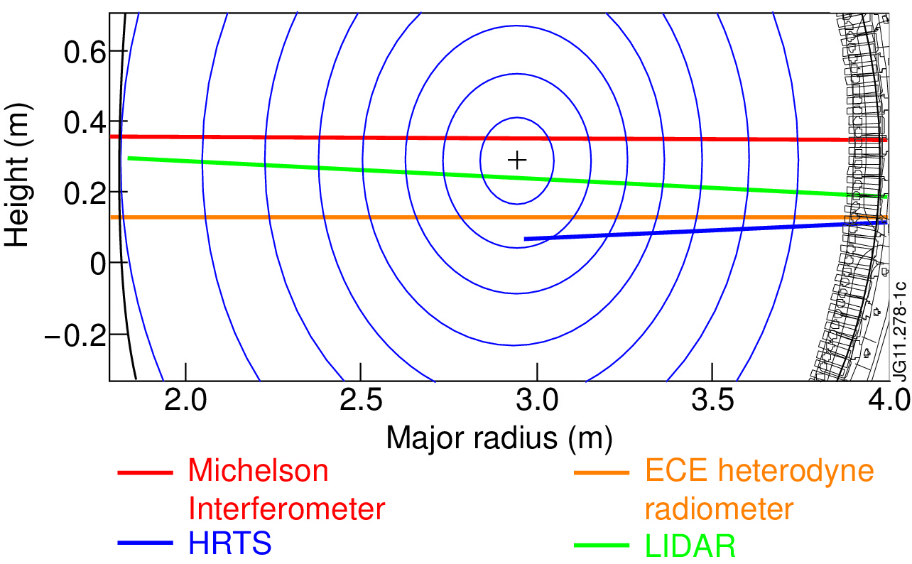
Figure 1: Line-of-sights of MICH, HRAD, LIDAR and HRTS for typical ohmic plasma (JPN 79853, t=5.0s). Flux surfaces are computed by EFIT.

The diagnostics’ lines-of-sight (LOS) are plotted in Fig. 1. For vessel configurations used between 1995 and 2009, MICH and LIDAR LOS are usually very close to the plasma midplane by a few $\mathrm{cm}$. HRAD and HRTS LOS are situated at lower z-position and usually miss the plasma centre. Mapped on the plasma midplane, HRAD $\mathrm{T_{e}}$ profiles usually exhibit a gap for $|\rho|<0.2$ and HRTS ones are restricted to the low field side ($\rho>0.2-0.3$), where $\rho=\pm\sqrt{\phi}$ and $\phi$ the normalised poloidal flux.

II.2 About ECE calibrations

MICH’s absolute calibration is used by HRAD and HRTS (for C20-C27); these diagnostics provide the JET $\mathrm{T_{e}}$ radial profiles with high time and radial resolutions that are usually shown in publications.

Absolute calibration of MICH follows, for each frequency $F$:

$$T_{\mathrm{keV}}(F)=I_{\mathrm{meas}}(F)/a(F)$$

with $I_{\mathrm{meas}}(F)$ the uncalibrated intensity measured by MICH and $a(F)$ the F-dependent calibration factors.

A radial calibration of the ECE system requires a magnetic reconstruction code (EFIT Lao et al. (1985); O’Brien et al. (1992)) that links the frequency domain of the observed ECE to the corresponding radial domain. The usual assumption of a cold ECE resonance is made, which means that $\omega_{n}=nq_{e}B_{0}/m_{e}$ i.e. all broadening effects, including relativistic ones, are neglected; see Ref Bekefi (1966) for a detailed analysis. This assumption results in a slight (a few $\mathrm{cm}$) artificial shift of the ECE $\mathrm{T_{e}}$ profiles in the outwards direction ($\mathrm{R_{ECE,\neq cold}<R_{ECE,cold}}$).

In order to update the (undocumented) 1996 ECE calibration in use for data measured between 1995 and 2010, a calibration campaign has been performed in 2007Zerbini (2007) and repeated for confirmation in 2010Schmuck (2011), addressing most of the issues raised in the conclusion of the 2007 campaign.

Both calibration campaigns indicate a small decrease of MICH’s sensitivity in the relevant ECE range ($90\text{\,}\mathrm{GHz}220\text{\,}\mathrm{GHz}$), causing (if applied) a $15-20\%$ increase of JET $\mathrm{T_{e}}$. Through cross-calibrations procedures (see (II.1)), HRAD and HRTS measurement would be affected similarly.

Following this revaluation, the periods of validity of the 1996, 2007 and 2010 ECE calibrations have been assessed. Data from MICH, HRAD and HRTS presented in this study still use the 1996 calibration. Applying the 2010 ECE calibration leads to a noticeable increase of $\mathrm{T_{e}}$ affecting the ECE TS ratio but not its variations.

II.3 Data

Data analysis mostly focuses on MICH and LIDAR measurements, which might be highly scattered: $\pm$5% for MICH and $\pm$10-15% for LIDAR. Time averaging is then required. JET pulses have been cut into timeslices of $1\text{\,}\mathrm{s}$ length where the total field ($\mathrm{B_{0}}$), plasma current ($\mathrm{I_{P}}$), additional power ($\mathrm{P_{ADD}}$), electron temperature and density ($\mathrm{T_{e}}$, $\mathrm{n_{e}}$) are kept reasonably constant: $\leq 1\%$ variations for $\mathrm{B_{0}}$, $\leq 5\%$ for $\mathrm{I_{P}}$, $\leq 10\%$ for central density, diamagnetic energy and additional power. All the plasma measurements presented in this paper are extracted from the JET public database.

In order to improve the readabiliy of the figures, temporal axes often represent timeslices instead of pulse dates or JPN. Timeslices selection is roughly linear with JPN as pulses usually have 5 to 10 timeslices with ohmic conditions, and not linear with pulse date. This choice is relevant as long term variations of plasma measurements (usually $\mathrm{T_{e}}$) are then easily seen.

All JET pulses between $35000<=\text{JPN}<=79853$ are included in the forthcoming analyses, where JPN 35000 was produced in May 1995 and JPN 79853 is the last pulse of C27 in November 2009. Pulse selection (pulses/timeslices) is done on plasma parameters as detailed in (III.2), providing of course that pulses were not plasma-free and that the ECE and TS diagnostics were operating.

Routines performing the data processing for all diagnostics, including ECE and TS as well as all other JET data, are constantly improved, which usually implies some data reprocessing. JET data used and shown in this study have been taken as stored in JET public database during Summer 2011 and no specific reprocessing was performed.

II.4 Magnetic mapping

Temperature profiles in tokamaks are four dimensional quantities (three radial, one temporal). The assumption of toroidal symmetry reduces the radial dimensions to two. Comparing measurements from different diagnostics, each having a different LOS, requires to map their geometrical LOS to the midplane plasma radius (or any other one) by using a magnetic equilibrium model; EFIT Lao et al. (1985); O’Brien et al. (1992) is used in this paper with a magnetic reconstruction only constrained by JET magnetic coils.

Discussing the accuracy of JET ECE radial position of all JET data studied in this paper is definitely out the scope of this paper. The hypothesis of cold resonance brings a slight overestimation of ECE radial position – a few $\text{\,}\mathrm{cm}$ for usual JET plasma conditions. Mapping of LOS to the central midplane affects it as well; more generally, JET ECE radial position relies on magnetics measurements.

Accuracy of JET magnetic measurements is $1.5\%$ . Following RefMurari et al. (2011) it leads to an accuracy of $1\text{\,}\mathrm{cm}1.5\text{\,}\mathrm{cm}$ for the magnetic geometric boundaries (for $\rho=1$) as computed by EFIT. Magnetics measurements are not yet constraining EFIT enough when reconstructing the magnetic equilibrium’s radial position for central regions of the plasmas, radial accuracy at the plasma core is not expected to be better than $\scriptstyle\sim$5-$10\text{\,}\mathrm{cm}$.

Radial localisation of ECE measurement depends on $\mathrm{B_{0}}$, following $\Delta r/r=\Delta B/B$ for cold resonance hypothesis, $r$ being the plasma major radius. This $\mathrm{B_{0}}$-related uncertainty leads to $\delta r$ $\scriptstyle\sim$$5\text{\,}\mathrm{cm}$ in the plasma centre. Taking only into account this (quite large) source of radial uncertainty stresses the complexity of the problem.

It is expected that these large uncertainties affecting the estimation of JET ECE radial position will not show clear trends of drifts with time, and that they are more likely to have the same effect as a low-amplitude white noise on $\mathrm{T_{e}}$ observables (see (II.5)).

Measurement position of LIDAR and HRTS are calibrated during JET shutdown and do not rely on EFIT on their LOS; they do though when mapping to the plasma midplane to be able to compare them to ECE $\mathrm{T_{e}}$ profiles.

II.5 Comparing $\mathrm{T_{e}}$ measurements

II.5.1 $\mathrm{T_{e}}$ observables

Different quantities can be defined to reduce the bi-dimensional profiles to one single value: they are called observables and are designed to quantify the discrepancies between MICH and LIDAR. Some possibilities have been studied:

• radial averaging around the plasma centre:

  $$\mathrm{\mathrm{T_{e}}_{\scriptscriptstyle MAX}}=\text{median}\left(\mathrm{T_{e}}(\rho,t)),|\rho|<0.2\right)$$

• integrals of $\mathrm{T_{e}}(\rho)$ over $\rho$ where measurements were available for both diagnostics:

  $$\mathrm{\mathrm{T_{e}}_{\scriptstyle{\scriptscriptstyle-}0.4\mapsto 0.9}}=\int_{-0.4}^{0.9}\mathrm{T_{e}}(\rho)\text{d}\rho$$

• $\mathrm{T_{e}}$ values for fixed $\rho$ values: $\mathrm{\mathrm{T_{e}}_{0.5}}$, $\mathrm{\mathrm{T_{e}}_{0.8}}$ and $\mathrm{\mathrm{T_{e}}_{0.9}}$ for, respectively, $\rho=0.5$, 0.8 and 0.9.

In order to reduce the uncertainties caused by a non-ideal midplane mapping (see (II.4)), profiles are radially averaged over the plasma centre, following $\mathrm{\mathrm{T_{e}}_{\scriptscriptstyle MAX}}$. This method has been thoroughly tested and it is regarded as robust, satisfyingly dealing with high- or low-peaked profiles as well as mapping issues around the plasma centre.

Using $\mathrm{\mathrm{T_{e}}_{\scriptstyle{\scriptscriptstyle-}0.4\mapsto 0.9}}$ or $\mathrm{\mathrm{T_{e}}_{0.5}}$ instead of $\mathrm{\mathrm{T_{e}}_{\scriptscriptstyle MAX}}$ would lead to very similar behaviour (variations and amplitudes). Mapping errors and measurement noise prevent $\mathrm{\mathrm{T_{e}}_{0.8}}$ and $\mathrm{\mathrm{T_{e}}_{0.9}}$ to be give similar results.

III Long-term observations of ECE TS ratio

III.1 Definition of ECE TS ratio

Stability of JET electron temperature is based on observations of $\mathrm{\mathrm{T_{e}}_{\scriptscriptstyle MAX}}$ as measured by MICH and LIDAR, i.e. $\mathrm{\mathrm{T_{e}}_{\scriptscriptstyle MAX,{\textsc{\footnotesize MICH}}}}$/$\mathrm{\mathrm{T_{e}}_{\scriptscriptstyle MAX,{\textsc{\footnotesize LIDAR}}}}$; this ratio is called ECE TS ratio.

The following paragraphs explain why HRAD and HRTS are not used to build an equivalent ECE TS ratio.

HRAD data is calibrated for each pulse against MICH, defining cross-calibration factors $\mathrm{\mathrm{T_{e}}_{\scriptscriptstyle MICH}}/\mathrm{\mathrm{T_{e}}_{\scriptscriptstyle HRAD}}$: any drift of MICH calibration could then be checked against these HRAD cross-calibration factors, provided the time stability of HRAD calibration is assessed independently. Despite our efforts, it has not been possible to use these HRAD cross-calibration factors to check MICH stability, as the former are obviously not stable enough to be used as references. Gaps in the cross-calibration factors can be explained by the waveguide switches that allow to select O- or X- microwave mixers that actually have moving parts; large time drifts observed in these cross-calibration factors (up to 96 for the latest set-up) do not all show similar features and each frequency channel appears to be almost independent from the other ones.

HRAD should therefore be regarded in this paper as an upgrade of MICH, with higher time and radial resolution. Two points make MICH best suited than HRAD for the ECE TS ratio; first: MICH LOS is closer to the plasma centre than HRAD’s; second: HRAD cross-calibration might add additional uncertainty when estimating $\mathrm{T_{e}}$.

The main reasons to prefer LIDAR to HRTS to build the ECE TS ratio are, first, the late availability of HRTS (Spring 2008) and, then, the dependence of HRTS calibration to HRAD, then MICH, for all the data presented in this paper.

For those reasons, ECE TS ratio is made of MICH and LIDAR data.

III.2 About data sets

Many plasma parameters can affect $\mathrm{T_{e}}$, the most obvious probably being the amount of additional power coupled to the plasma. For non purely Ohmic pulses, a selection of pulses/timeslices has been made on $\mathrm{P_{ADD}}=\mathrm{P_{NBI}}+\mathrm{P_{ICRH}}$, where $\mathrm{P_{NBI}}$ is the total additional power from NBI (Neutral Beam Injection) and $\mathrm{P_{ICRH}}$ is the total additional power from ICRH (Ion Cyclotron Radio-frequency Heating). Pulses with LHCD (Lower Hybrid Current Drive) are not included in the analysis because this heating system affects ECE signals, especially at the plasma edge.

The following arbitrary separation on $\mathrm{P_{ADD}}=\mathrm{P_{NBI}}+\mathrm{P_{ICRH}}$ is then used:

• Ohmic pulses with $\mathrm{P_{ADD}}=$$0\text{\,}\mathrm{MW}$

• “Low-power” pulses with $\mathrm{P_{ADD}}$=$010\text{\,}\mathrm{MW}$

• “High-power” pulses with $\mathrm{P_{ADD}}$=$1020\text{\,}\mathrm{MW}$

Low-power pulses are mostly in L-mode while high-power ones are mostly in H-mode; no distinction is actually made between both confinement modes in this paper.

Two data sets are defined:

• The “large data set” spans 15 years of data produced in JET (1995-2009) with a broad selection of plasma parameters. This set gives an overview of the ECE TS ratio, i.e. how $\mathrm{T_{e}}$ measurements from ECE (MICH) and TS (LIDAR) systems compare with time.

• The “reference data set” spans 13 years of data produced in JET (1998-2009) with narrow selections of plasma parameters (e.g. $\mathrm{B_{0}}$ = $2.41\text{\,}\mathrm{T}$, $\mathrm{I_{P}}$ = $1.96\text{\,}\mathrm{MA}$); 18 parameters are checked and selected to be as constant as possible. These pulses are then regarded as “beacon” or “reference” pulses, allowing for more precise study of ECE TS variations with time.

III.3 Large data set: 1995-2009

III.3.1 Description

JET data has been analysed from 1995 to 2009 for $35000<=\text{JPN}<=79853$ where both MICH ad LIDAR were on-line. Data selection is limited on $\mathrm{B_{0}}$ and $\mathrm{I_{P}}$ with $\mathrm{B_{0}}$ limited to $23\text{\,}\mathrm{T}$ and $\mathrm{I_{P}}$ to $1.54\text{\,}\mathrm{MA}$; and after additional power separation:

Ohmic:	15k pulses	135k timeslices
Low-power:	6k pulses	23k timeslices
High-power:	3k pulses	10k timeslices

III.3.2 Observations: 1995-2009

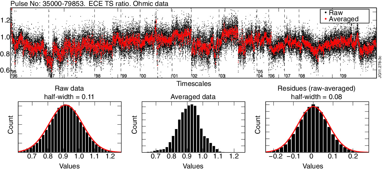
Figure 2: ECE TS ratio for ohmic pulses, large data set, 1995-2009.
(Top) Data in black, 50-timeslices average in red. Years are indicated
(Bottom-left): distribution of ECE TS ratio data, with a half-width of 0.11 and Gaussian fit in red.
(Bottom-centre): distribution for 50-timeslices average.
(Bottom, right): distribution of residues, defined as ECE TS ratio minus averaged ones, with a half-width of 0.08. Gaussian fit in red

In Fig. 2, the ECE TS ratio is plotted for ohmic conditions. Raw data ranges from 0.5 to 1.25 and its distribution is Gaussian-like (Fig. 2, bottom, left) with a mean around 0.95 and a half-width of 0.11. Averaged data are shown as well, over 50 timeslices that usually represents 5-10 pulses; distribution clearly departs from Gaussian (Fig. 2, bottom, centre) and residues look like white noise (null mean Gaussian-like distribution, Fig. 2, bottom, right) with a 0.08 half-width. Evolution patterns are obviously noticeable on raw and averaged data.

Focusing on averaged data, ECE TS ratio shows very clear structures roughly centered on $\scriptstyle\sim$0.95 with $\scriptstyle\sim$$20\%$ temporal variations (peak-to-peak).

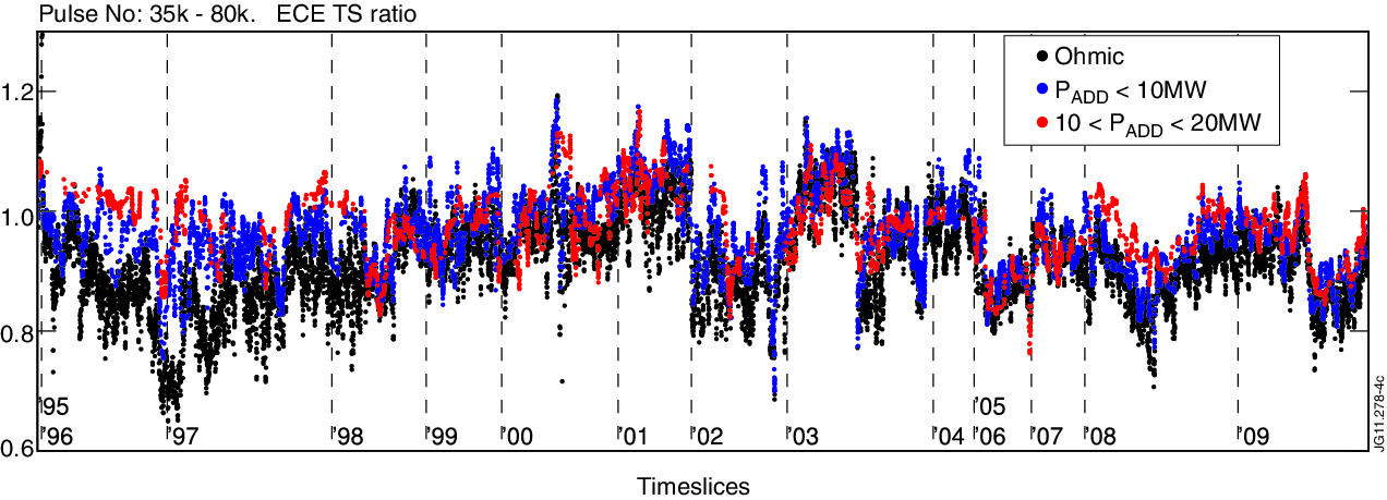
Figure 3: ECE TS ratio against timeslices for the large data set, 1995-2009. Ohmic data in black (15k pulses, 135k timeslices), low-power in blue ( ${0}\!<\!\mathrm{P_{ADD}}\!<\!{10}$ MW, 6k pulses, 23k timeslices), high-power in red (${10}\!<\!\mathrm{P_{ADD}}\!<\!{20}$ MW, 3k pulses, 10k timeslices). Years are indicated by dashed lines.

Ohmic, low-power and high-power plasma conditions are plotted in Fig. 3, for averaged data as previously defined. The three data sets mostly exhibit the same trends and a very good agreement after 1998. Compared with the ohmic set, the ECE TS ratio is sometimes slightly higher for high-power plasma conditions, reaching 10% between 2007 and 2009 and even 15% between 1995 to 1998. A slight offset might be observed between ohmic and non-ohmic data.

Focusing on the ohmic data set, Fig. 2 and Fig. 3 show the same variations of the ECE TS ratio, that appear to be without clear trends. Large drops of $\raise 0.73193pt\hbox{$\scriptstyle\sim$}20\%$ are observed in 1997, 2001, 2003 and 2009. Numerous increasing or decreasing trends whose amplitudes amount to 10-20% can be seen, spanning large numbers of timeslices (thousands of them, say typically a few months); less sudden variations are also observed.

Data selection is very broad and spans almost fifteen years. ECE TS ratio exhibits many sudden changes; explaining the precise causes of most of those changes is out of the scope of this paper. For instance, different vessel configurations have been used in JET including the various divertor, different operation modes, differently shaped plasmas etc. It has been checked that these changes of divertor configuration do not correspond with any obvious evolution of the ratio.

III.3.3 Observations: C20-C27, 2008-2009

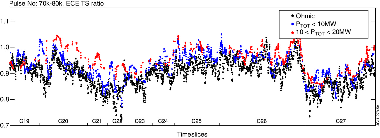
Figure 4: ECE TS ratio against timeslices for large data set limited to C20-C27, 2008-2009, i.e. 5800 pulses, 41k timeslices. Ohmic data in black low-power in blue ( ${0}\!<\!\mathrm{P_{ADD}}\!<\!{10}$ MW), high-power in red (${10}\!<\!\mathrm{P_{ADD}}\!<\!{20}$ MW). Data are averaged over 50 timeslices. JET campaigns are indicated.

ECE TS ratio shown in Fig. 4 is for a time selection limited to the JET campaigns between 2008 and 2009 (C20-C27, $72000<=\text{JPN}<=79853$). When available, HRAD and HRTS data have been selected as well – but not shown in Fig. 4.

Like Fig3, ECE TS ratio shows $\pm$13% variations within [0.8-1.05], with the same strong evidence of evolution patterns well outside a $\scriptstyle\sim$8% near-normal scattering. Ohmic, low-power and high-power wide sets show almost the same evolutions and levels (ohmic and low-power only) for the ratio, whereas the high-power ones have a slightly higher level in some case, up to 10% for C20.

III.3.4 Key points

This is one of the main conclusion of the paper: between 1995 and 2009, the (temporal) stability of ECE TS ratio can not be guaranteed, even for short time-period (say a few months), as shown in Fig. 2 and Fig. 3; $\mathrm{T_{e}}$ measurements of MICH and LIDAR do not compare well, even on averaged data. This point is regarded as a problematic one from a data coherence point-of-view, as this ratio is expected to stay around 1.0 with some reasonable margins.

Large-scale drifts of the ECE TS ratio can obviously not been explained satisfactorily by monotonic drifts of ECE or LIDAR calibrations. This point will be discussed more thoroughly (mostly in (V)).

III.4 1998-2009 reference pulses

ECE TS ratio variations previously detailed for the large data set might be explained by variations of one or many plasma parameters. In order to identify possible cause-and-effect links, a first step is to select pulses with plasma conditions kept as constant as possible.

III.4.1 Description

As such dedicated reference pulses have been neither designed nor performed through the years, a few sets of plasma conditions have been chosen and flagged as being used as reference pulses: recovery or cleaning pulses with a long enough Ohmic phase ($3\text{\,}\mathrm{s}$). Usually performed for the machine to recover from a disruption, they are usually made on a daily or weekly basis and do have very similar conditions through the years. These recovery pulses were not designed to be fully reproducible, e.g. the impurities deposits displaced by the disruption they are recovering from are expected to affect the plasma composition, but no better pulses sets have been found.

Likewise, references pulses were not designed to maintain a constant $\mathrm{T_{e}}$.

Signal		Average	$\pm$ dev.	in %
$\mathrm{B_{0}}$ [$\mathrm{T}$]		2.41	$\pm$0.01	(0.4%)
$\mathrm{I_{P}}$ [$\mathrm{MA}$]		1.96	$\pm$$1.2\text{\times}{10}^{-2}$	(0.6%)
$\mathrm{P_{OHM}}$ [$\mathrm{MW}$]		0.81	$\pm$0.52	(65%)
$\mathrm{W_{DIA}}$ [$\mathrm{MJ}$]	($\star$)	0.90	$\pm$$5.4\text{\times}{10}^{-2}$	(6%)
$\mathrm{ne_{0}}$ [$1\text{\times}{10}^{19}\text{\,}\mathrm{m}^{-3}$]		2.24	$\pm$0.27	(12%)
$\mathrm{P_{e0}}$ [$\mathrm{kPa}$]		6.80	$\pm$2.0	(29%)
$\mathrm{\mathrm{T_{e}}_{\scriptscriptstyle MAX,{\textsc{\footnotesize MICH}}}}$ [$\mathrm{keV}$]		2.00	$\pm$0.28	(14%)
$\mathrm{\mathrm{T_{e}}_{\scriptscriptstyle MAX,{\textsc{\footnotesize LIDAR}}}}$ [$\mathrm{keV}$]		2.17	$\pm$0.35	(16%)
$\mathrm{Z_{EFF}}$		1.99	$\pm$0.69	(35%)
$\beta_{n}$	($\star$)	0.38	$\pm$$2.4\text{\times}{10}^{-2}$	(6%)
$\mathrm{l_{i}}$	($\star$)	1.19	$\pm$$3.7\text{\times}{10}^{-2}$	(3%)
$\mathrm{q_{95\%}}$	($\star$)	3.67	$\pm$0.21	(6%)
plasma volume [$\mathrm{m}^{3}$]	($\star$)	80.7	$\pm$1.80	(2%)
triangularity (upper)	($\star$)	0.14	$\pm$$8.3\text{\times}{10}^{-2}$	(57%)
triangularity (lower)	($\star$)	0.18	$\pm$0.07	(39%)
elongation	($\star$)	1.56	$\pm$0.12	(7%)
midplane centre r-pos [$\mathrm{m}$]	($\star$)	2.94	$\pm$$1.1\text{\times}{10}^{-2}$	(0.3%)
midplane centre z-pos [$\mathrm{m}$]	($\star$)	0.31	$\pm$$2.3\text{\times}{10}^{-2}$	(7%)

Table 2: Plasma parameters for reference data set, limited to $58632<\text{JPN}<79645$, 05/03/03 to 14/10/09, 5702 timeslices, 331 pulses.
($\star$): data computed by EFIT.

As detailed in Table 2 where typical ranges of main plasma parameters are listed, 331 reference pulses have been manually selected for $58300<\text{JPN}<79853$ (2003-2009) corresponding to 5702 timeslices. For dates prior to 2003, very few pulses could be found with $\mathrm{B_{0}}$ = $2.41\text{\,}\mathrm{T}$ and $\mathrm{I_{P}}$ = $1.96\text{\,}\mathrm{MA}$.

Some signals are strongly scattered or show non-negligible variations: Ohmic power ($\mathrm{P_{OHM}}$), central electron density ($\mathrm{n_{e}}_{0}$), central electron pressure ($\mathrm{P_{e0}}$), effective charge ($\mathrm{Z_{EFF}}$), plasma triangularities and $\mathrm{\mathrm{T_{e}}_{\scriptscriptstyle MAX}}$ from MICH and LIDAR. Besides $\mathrm{\mathrm{T_{e}}_{\scriptscriptstyle MAX}}$, the only measured signals showing remarkable trends are the vacuum field ($\pm$0.4%) with similar variations as the total field, and $\mathrm{Z_{EFF}}$ ($\pm$25%).

III.4.2 Observations

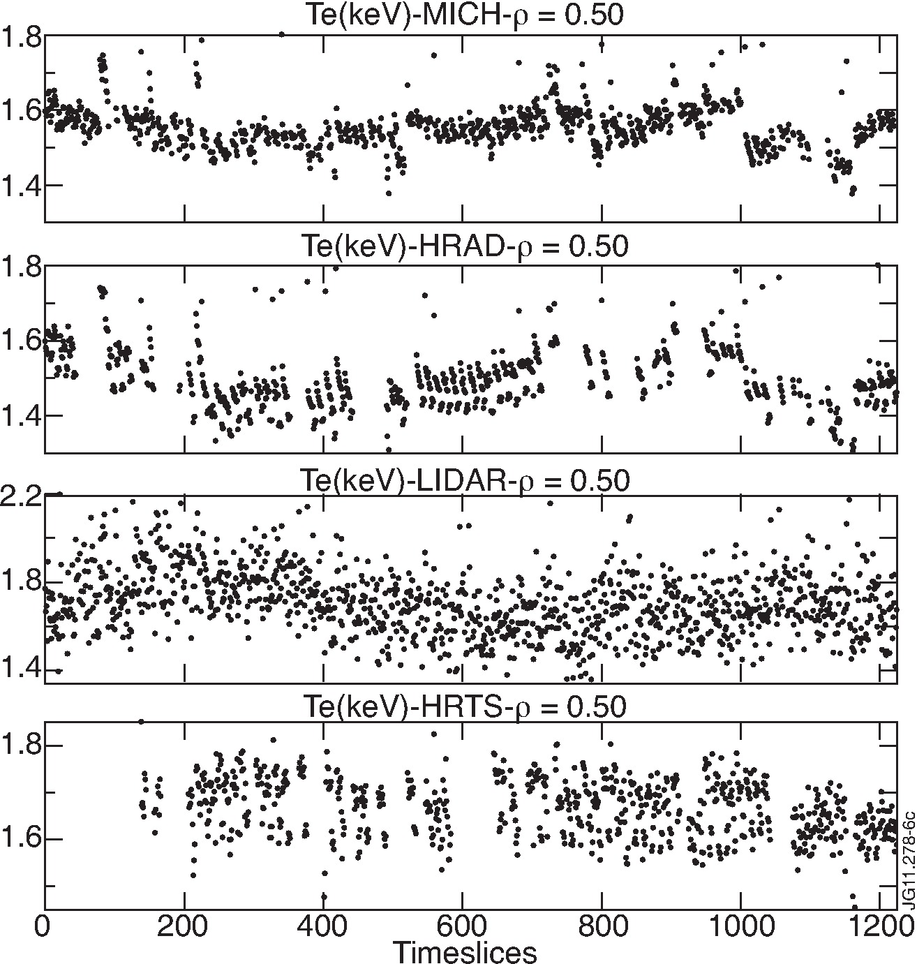
Figure 5: Electron temperature measurements ($\mathrm{keV}$, $\rho=0.5$) against timeslices for reference data set as described in Table 2, limited to C20-27 pulses: 124 pulses and 1227 timeslices selected. Measurement from different diagnostics are shown: MICH, HRAD, LIDAR and HRTS.

As shown in Fig. 5, four diagnostics are available for C20-C27 campaigns: MICH, LIDAR, HRAD and HRTS, for $\rho=0.5$. Each diagnostic shows similar variations for different radial positions $\rho=[0.2,0.3,0.5]$, even if these variations are not always similar from one diagnostic to another. Pulse-to-pulse cross-calibration makes HRAD follow MICH very closely, as expected. Even if HRTS is cross-calibrated against HRAD for the whole C20-C27 period (see (II.1)), variations of both measurements do not appear to be linked. Note that LIDAR and HRTS exhibit different variations, even if their measurements are from the same physics basics.

As shown in Fig. 5, $\mathrm{T_{e}}$ is obviously not constant for the reference set: no reference temperature can then be used to assess the stability of diagnostics. Similarities between the ECE TS ratio and $\mathrm{\mathrm{T_{e}}_{\scriptscriptstyle MAX,{\textsc{\footnotesize MICH}}}}$ and $\mathrm{\mathrm{T_{e}}_{\scriptscriptstyle MAX,{\textsc{\footnotesize LIDAR}}}}$ are to be expected, but depending on the pulse range, trends have features sometimes linked to $\mathrm{\mathrm{T_{e}}_{\scriptscriptstyle MAX,{\textsc{\footnotesize MICH}}}}$ variations and sometimes $\mathrm{\mathrm{T_{e}}_{\scriptscriptstyle MAX,{\textsc{\footnotesize LIDAR}}}}$: again, no firm conclusion can be drawn on the cause of those drifts.

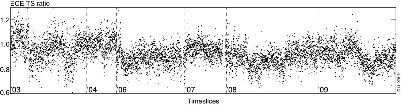
Figure 6: ECE TS ratio against timeslices for reference data set as described in Table 2. Years are indicated by dashed lines.

The ECE TS ratio for reference pulses is plotted in Fig. 6. As in (III.3.2), residues have a near-normal (Gaussian-like) distribution similar to the one obtained for the large data set – with the mean around 0.95 and non-negligible scattering (=half-width) of 0.1. Peak-to-peak amplitude is slightly above 30%.

ECE TS ratio drifts and variations are found to be in agreement with the large sets (Fig. 3) and Pearson’s cross correlation coefficient between ratios from both sets is quite high: around 0.7 for $\text{JPN}>54500$ (from 2003 to 2009) as well as for C19-C27 ($\text{JPN}>70000$).

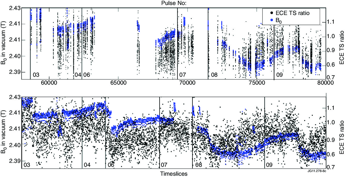
Figure 7: ECE TS ratio (left y-axis, black) and vacuum magnetic field ($\mathrm{B_{0}}$, right y-axis, blue) against JPN (top) and timeslices (bottom) for reference data set as described in Table 2. Years are indicated by lines.

As stated previously, $\mathrm{B_{0}}$ and $\mathrm{Z_{EFF}}$ are the only measurements (other than $\mathrm{T_{e}}$) showing noticeable trends. $\mathrm{Z_{EFF}}$ does not show any variations similar to the ECE TS ratio, yet. In Fig. 7, magnetic field (measured by Rogowskii coils) show large-scale drifts similar to the ones observed for ECE TS ratio, but the observed $\mathrm{B_{0}}$ variations have a very low amplitude, around $\pm$0.4%; note that these experimental variations are below the uncertainty level of KC1D integrator measurement (1.5%, see (II.4)).

As stated in (II.1) and shown in Fig. 1, MICH and LIDAR LOS are not similar, both missing the plasma center by $\scriptstyle\sim$$5\text{\,}\mathrm{cm}$ according to EFIT reconstruction. For reference pulses, r- and z-position are observed to move by approximately 2-$3\text{\,}\mathrm{cm}$ at most (see Table 2). Note that from (II.4) these values are believed to be within the uncertainties of EFIT reconstruction in the plasma center. Even if those displacements are regarded as real, $\mathrm{T_{e}}$ profiles in usual JET plasmas as like for the (ohmic) reference pulses are not peaked enough to explain this 30% peak-to-peak variations. Furthermore, measurements are actually volume-averaged for both MICH (usually a few $\text{\,}\mathrm{cm}$) and LIDAR ($\scriptstyle\sim$$1\text{\,}\mathrm{cm}$).

III.4.3 Key points

For reference pulses, variations of ECE TS ratio appear to be mostly disconnected from the variations observed on the 18 plasma parameters described in Table 2, except for the very low amplitude variations of $\mathrm{B_{0}}$.

About the similar long-term drifts shown by $\mathrm{B_{0}}$ and ECE TS ratio (Fig. 7), variations amplitudes differ from more than one order of magnitude: $\pm$0.4% for $\mathrm{B_{0}}$ and $\pm$15% for ECE TS ratio. Yet long-term trends of both quantities show a reasonably good agreement. But $\mathrm{B_{0}}$ variations do not affect the computation of $\mathrm{\mathrm{T_{e}}_{\scriptscriptstyle MAX,{\textsc{\footnotesize MICH}}}}$ and $\mathrm{\mathrm{T_{e}}_{\scriptscriptstyle MAX,{\textsc{\footnotesize LIDAR}}}}$. For ECE diagnostics, frequency-position mapping adds radial uncertainties following $\Delta r/r$ $\scriptstyle\sim$$\Delta B/B$: $\pm$0.4% for $\mathrm{B_{0}}$ converts then to $\pm$1-$1.5\text{\,}\mathrm{cm}$ at the plasma centre (R$\scriptstyle\sim$$3\text{\,}\mathrm{m}$), which is below the expected uncertainties caused by the midplane mapping.

From these two points, the expected impact of $\pm$0.4% $\mathrm{B_{0}}$ variations on $\mathrm{\mathrm{T_{e}}_{\scriptscriptstyle MAX}}$ are considered as negligible – and vice versa. ECE TS ratio and $\mathrm{B_{0}}$ long-term drifts show then a good agreement between 2003 and 2009, but no direct cause-and-effect link between both can be thought of by the authors.

A possible cause for $\mathrm{B_{0}}$ variations is described and analysed in the next section.

IV Observation of seasonal patterns

IV.0.1 Description

In JET, magnetic field signals (pick-up coils, loops, Rogowskii coils) used to build $\mathrm{B_{0}}$ are all recorded by the same type of 8-channel isolated integrator (referred as KC1D integrator) used for the principal magnetic dagnostics. When those KC1D integrators were installed in August 1994 there was some concern as to how the inner capacitors would age and perform with respect to temperature. To estimate the extent of these effects, a very stable test-signal generator was permanently installed in KC1D and connected to the 8 channels of a KC1D integrator sample Horton (2005). For each pulse, the data from this module are taken and stored as if they were real coil signals.

IV.0.2 Observations

The off-plasma signals of KC1D integrator are plotted in Fig. 8. Seasonal drifts are observed, as stated in the reportHorton (2005): “Up until the JET 2000/2001 shutdown, channels 2 to 8 show cyclic variation of about $\pm$0.1%, which appear to follow winter-summer pattern”. The cyclic variations observed were considered to be temperature effects on these capacitors, but this point has not been studied further.

Figure 8: KC1D integrator test against years. Expected values = 26214 bits, drift amplitude = 120 bits = $\sim 0.2\%$ variations.

As plasma measurements of $\mathrm{B_{0}}$ are performed with the same type of integrators, they are then expected to suffer the same seasonal variations. As shown in Fig. 9, $\mathrm{B_{0}}$ shows variations quite well matched by KC1D integrator measurements for the time period mid-2002 to 2009. Amplitudes are quite similar: around $\pm$0.4% for $\mathrm{B_{0}}$ and around $\pm$0.2% for KC1D integrator drifts. The agreement is quite poor for the 1998-2000 time period.

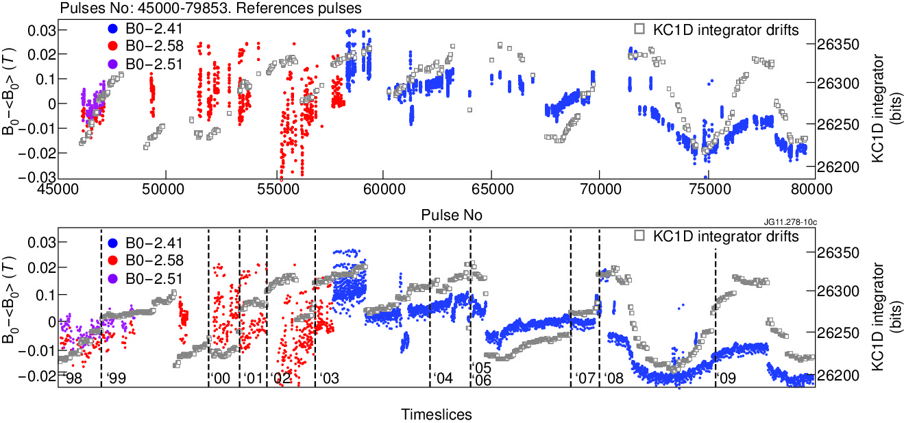
Figure 9: Variations of vacuum toroidal field ($\mathrm{B_{0}}$, left y-axis, full symbols) and KC1D integrator drifts (right y-axis, open symbols, bits-26000) against JPN (top) and timeslices (bottom) for references data set as described in Table 2. Additional data sets with similar plasma conditions are shown, for $45000<\text{JPN}<58632$ with different $\mathrm{B_{0}}$ values: $2.41\text{\,}\mathrm{T}$ in blue, $2.51\text{\,}\mathrm{T}$ in magenta, $2.58\text{\,}\mathrm{T}$ in red. Years are indicated by dashed lines.

IV.0.3 Key points

Given the similarity of $\mathrm{B_{0}}$ and KC1D integrator variations, in terms of amplitude and temporal drifts, it is likely that $\mathrm{B_{0}}$ variations observed in Fig. 7 and Fig. 9 after mid-2002 should not been accounted for real events taking place in JET plasmas.

Note that those off- and on-plasma variations affecting the field measurements are below their experimental uncertainty (1.5%, (II.4)).

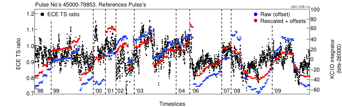
Figure 10: ECE TS ratio (left y-axis, black) and KC1D integrator drifts (right y-axis, blue) against timeslices for references data set as described in Fig. 9. KC1D integrator drifts values, slightly re-scaled and shifted (offsets $<20$ bits), are in red. Years are indicated by dashed lines.

As stated in (III.4) (Fig. 6), the only plasma parameter showing variations correlated with ECE TS ratio for the reference pulses is $\mathrm{B_{0}}$. The causality of the link between (on-plasma) ECE TS ratio and (off-plasma) KC1D integrators tests can not be established from the available data, or the possibility of a common but still unknown cause having similar effects on both signals. Seasonal variations of external temperature at JET site are yet regarded as the main suspect of the long-term drifts of ECE TS ratio after mid-2002 and since 2009. Little can be said between 1995 and mid-2002.

Daily variations of JET site temperature might also well trigger similar effects. The corresponding analysis has been made and does not show any effect on ECE TS ratio above a $1\%$ uncertainty, even for the warmer days/months when the night/day temperature variations reach up to $15\,^{\circ}\!\textrm{C}$ – quite uncommon for Oxfordshire. Time constants considered here are consequently more likely to be of the order of weeks or months than days.

V Long-term stability of Michelson interferometer

Another way of explaining the observed variations of ECE TS ratio is to directly check the variations of $\mathrm{\mathrm{T_{e}}_{\scriptscriptstyle MICH}}$ and $\mathrm{\mathrm{T_{e}}_{\scriptscriptstyle LIDAR}}$, but even for the reference data set that is more “constrained” than the large data set, no other $\mathrm{T_{e}}$ measurement can be used as a reference to assess MICH and LIDAR stability. The idea developed in this section is to check MICH stability with the in-lab (i.e. off-plasma) monitoring performed throughout the years.

V.1 In-lab measurements

In order to check the stability of MICH, in-lab calibrations are routinely performed every few months using a calibrated hot source since the early years of JET (1984); since 1996, the same hot source ($600\text{\,}\mathrm{\SIUnitSymbolCelsius}$, built by SPECAC in the 90s) has been used. Measurements on a cold source (liquid nitrogen) were performed but not sufficiently frequently (i.e. monthly). These measurements were performed by different MICH operators but as the set-up for in-lab calibrations is documented and reproducible, it is believed that these measurements were done in very similar ways.

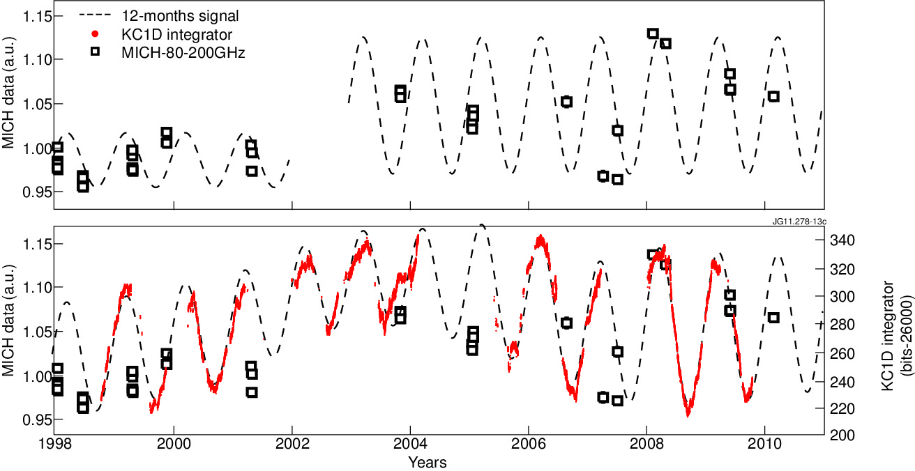
Figure 11: MICH in-lab measurements (left y-axis, squares) and KC1D integrator drifts (right y-axis, bottom, red points) against time for 1998-2010. Synthetic signals with a 12-month period (black dashed lines) are added on both plots.

Results of MICH in-lab measurements are reported in Fig. 11. All the measured interferograms have been reprocessed using the same routines and the resulting spectrograms have been integrated over the $80\text{\,}\mathrm{GHz}200\text{\,}\mathrm{GHz}$ band, which is most frequently used for measuring $\mathrm{T_{e}}$ with the second ECE harmonic in X-mode.

No cyclic pattern can be easily observed in Fig. 11. Data scattering is below $\pm$5% for 1998-2002 and below $\pm$10% for 2003-2010 which is at least twice lower than the scattering of ECE TS ratio. The scattering increase of MICH in-lab measurement around 2003 takes place approximately at the time where ECE TS ratio starts to be well correlated with the seasonal drifts of the off-plasma magnetics measurements – as shown in Fig. 10. The ECE TS ratio does not show such an increase of scattering.

V.2 Cryodetector bias voltage

The bias voltage of MICH’s cryodetector is provided by batteries delivering a very stable voltage ($7\text{\,}\mathrm{V}$ or $10\text{\,}\mathrm{V}$ depending on the battery model). Sensitivity of the cryodetector to this bias voltage has been characterised. Taking $10\text{\,}\mathrm{V}$ as a reference, detector sensitivity is slightly increased ($5\%$) for $7\text{\,}\mathrm{V}$ and decreased for lower voltages ($>10\%$ decrease below $4\text{\,}\mathrm{V}$). Sensitivity variations stay below $5\%$ for a bias-voltage from $610\text{\,}\mathrm{V}$. This voltage was monitored on a monthly basis and the consequences of three serious drops ($<6\text{\,}\mathrm{V}$) have been carefully examined. The expected impact on $\mathrm{\mathrm{T_{e}}_{\scriptscriptstyle MAX,{\textsc{\footnotesize MICH}}}}$ is a (possibly slow) $>10\%$ decrease, then a steep recovery when batteries are recharged. This signature has not been observed on JET data; the causality link between such uncontrolled variations of the MICH cryodetector bias voltage and the drifts of the ECE TS ratio is not established then.

V.3 Limits

This monitoring includes the MICH system, the cryodetector and some electronic components. DAQ (hardware) is different for in-lab and plasma measurements. The fifty meters of waveguide, the vessel windows and the antenna are not included in this monitoring.

Components that are included in the monitoring and are the more prone to suffer from external temperature variations are the cryodetector, which uses liquid helium, and the electronic amplifiers, which provided a $50\text{\,}\mathrm{dB}54\text{\,}\mathrm{dB}$ gain for plasma measurements and $80\text{\,}\mathrm{dB}$ for in-lab measurements and in-vessel calibrations. Their sensitivities to temperature variations ($\raise 0.73193pt\hbox{$\scriptstyle\sim$}15\,^{\circ}\!\textrm{C}$) have not been checked yet.

Propagation through the waveguide reduces the signal by $715\text{\,}\mathrm{dB}$, following an $\mathrm{F}^{2}$ scaling between $70\text{\,}\mathrm{GHz}$ and $350\text{\,}\mathrm{GHz}$. These values are not expected to vary with temperature. The in-vessel window certainly slightly modifies the EC signal, but should not cause any seasonal variations. The DAQ’s old electronics might be sensitive to temperature variations. These three points are possibly causing calibration drifts but their amplitudes are expected to remain quite small, and they are not expected to introduce any seasonal variations.

V.4 Key points

This monitoring was historically designed to check the time stability of MICH between in-vessel calibrations; tracking down such seasonal variations would require at least monthly measurements, which is not the case.

The main conclusion is that the available data from MICH monitoring does not show any 12-months cycles. Furthermore, data scattering of in-lab MICH calibration is a factor of two lower than observed on the ECE TS ratio.

Observed variations of in-lab measurements could come from:

• Experimental errors in the calibration process, like hot source position and temperature and different transmission in the open waveguide …but these will not affect $\mathrm{\mathrm{T_{e}}_{\scriptscriptstyle MICH}}$ measurement.

• MICH calibration drifts that will affect $\mathrm{\mathrm{T_{e}}_{\scriptscriptstyle MICH}}$ measurement, for example the modification of ageing amplifiers’ gain or evolution of the components of the cryogenic detector.

On the other hand, some other effects described in (V.3) and outside the monitoring scope could modify $\mathrm{T_{e}}$ measurements.

Although available data from MICH lab monitoring does not support the idea that MICH is mostly responsible for ECE TS ratio variations, lack of data prevents any firm conclusion to be drawn.

A possibility to definitely track down such calibration drifts would be to perform a full in-vessel ECE calibration on a monthly basis (at least), during 1 or 2 years. This is however not feasible on JET.

VI $\mathrm{W_{th}}$ estimations

VI.1 Description

Plasma thermal energy ($\mathrm{W_{th}}$) is estimated from the plasma pressure profiles, i.e. using the kinetic expressions following RefGarbet et al. (1992):

$$\mathrm{W_{th}} =\mathrm{W_{th,e}}+\mathrm{W_{th,i}}$$

$$\mathrm{W_{th,e}} =\frac{3}{2}\int{\mathrm{n_{e}T_{e}\ dV}}$$

$$\mathrm{W_{th,i}} \raise 0.73193pt\hbox{$\scriptstyle\sim$}\frac{7-\mathrm{Z_{EFF}}}{6}\mathrm{\frac{T_{i}}{T_{e}}}\mathrm{W_{th,e}}$$

Plasma density is taken from LIDAR measurements while $\mathrm{T_{e}}$ is measured by MICH ($\mathrm{W_{th,\scriptscriptstyle{\textsc{\footnotesize MICH}}}}$) and LIDAR ($\mathrm{W_{th,\scriptscriptstyle{\textsc{\footnotesize LIDAR}}}}$). Ion temperature is measured by charge exchange diagnosticVon Hellermann and Summers (1993).

Another way to estimate $\mathrm{W_{th}}$ uses magnetics measurements, defining then $\mathrm{W_{th,mag}}$:

$\mathrm{W_{th,mag}}=\mathrm{W_{DIA}}-\frac{3}{2}\mathrm{W_{fast,\perp}}$

where $\mathrm{W_{fast,\perp}}$ is the stored energy in the perpendicular component of the fast particle population, estimated from the computation of power deposition of ion cyclotron reasonance heating (ICRH) by PIONEriksson, Hellsten, and Willen (1993); Eriksson and Hellsten (1995) for NBI-only plasmas.

Comparing kinetic $\mathrm{W_{th,\scriptscriptstyle{\textsc{\footnotesize MICH}}}}$ and $\mathrm{W_{th,\scriptscriptstyle{\textsc{\footnotesize LIDAR}}}}$ to the diamagnetic $\mathrm{W_{th,mag}}$ provides information on the measurement accuracy of $\mathrm{T_{e}}$ by MICH and LIDAR. $\mathrm{W_{th}}$ is then estimated following both ways for purely NBI-heated plasmas from the wide set, for $\mathrm{P_{NBI}}$ $>5\text{\,}\mathrm{MW}$.

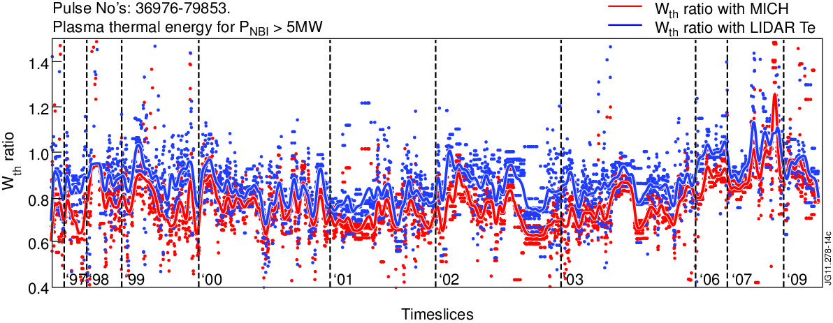
Figure 12: Ratio of (kinetic) $\mathrm{W_{th}}$ to (magnetics) $\mathrm{W_{th,mag}}$ with MICH (red) and LIDAR (blue) $\mathrm{T_{e}}$ profiles in $\mathrm{MJ}$ against timeslices for references data set. Data selection from JPN =36857 to 79853 with $\mathrm{P_{NBI}}$ $>5\text{\,}\mathrm{MW}$, 672 pulses selected, 2604 timeslices. Smaller points represent raw data, bigger points represent smoothed data. Years are indicated by dashed lines.

VI.2 Observations

Estimations of $\mathrm{W_{th,\scriptscriptstyle{\textsc{\footnotesize MICH}}}}/\mathrm{W_{th,mag}}$ and $\mathrm{W_{th,\scriptscriptstyle{\textsc{\footnotesize LIDAR}}}}/\mathrm{W_{th,mag}}$ are shown in Fig. 12. Large similarities are observed between both kinetics estimations and they clearly depart from the diamagnetic one, with variations between -40% and 10%. Most of the time $\mathrm{W_{th,\scriptscriptstyle{\textsc{\footnotesize MICH}}}}<\mathrm{W_{th,\scriptscriptstyle{\textsc{\footnotesize LIDAR}}}}$, coherent with the observations of ECE TS ratio shown in Fig. 2 and Fig. 3: consequently $\mathrm{W_{th,\scriptscriptstyle{\textsc{\footnotesize LIDAR}}}}$ estimation is generally slightly closer to the diamagnetic $\mathrm{W_{th}}$ than $\mathrm{W_{th,\scriptscriptstyle{\textsc{\footnotesize MICH}}}}$. No other systematic trend is observed.

The same exercise has been done for three other cases: first with purely Ohmic plasma where $\mathrm{W_{th}}=\mathrm{W_{DIA}}$ on a larger pulses database, and then with a condition on plasma central density for the NBI-only plasmas (central $\mathrm{n_{e}}_{0}$ $<5\text{\times}{10}^{19}$ $\mathrm{m}^{-3}$ and $\mathrm{n_{e}}_{0}$ $>5\text{\times}{10}^{19}$ $\mathrm{m}^{-3}$) to check the impact of density on the $T_{i}$ measurements. These additional cases lead to very similar conclusions as the ones drawn for the NBI-only case.

VI.3 Key points

The comparison of kinetic or diamagnetic estimations of $\mathrm{W_{th}}$ does not provide any definitive information on the accuracy of MICH or LIDAR measurements. It seems that MICH is slightly under-estimating $\mathrm{T_{e}}$, but both of them lead to a $\mathrm{W_{th}}$ generally 20-30% below the diamagnetic $\mathrm{W_{th}}$, for both Ohmic and NBI-only plasmas.

VII ECE TS radial discrepancies

VII.1 Description

Relatively low signal-to-noise ratio and lower radial definition of LIDAR $\mathrm{T_{e}}$ profiles make it impossible to satisfyingly track down ECE TS position errors. Radially well-defined profiles measured by HRTS are routinely available since April 2008 (JPN $\scriptstyle\sim$72000, from C20). After midplane mapping, they can be compared to the high time and high (radial) resolution HRAD profiles.

A long lasting issue within the JET community is that HRAD and HRTS profiles are not always similar (e.g. as described in Refde la Luna et al. (2003); Barrera, de la Luna, and Contributors (2008)); these mismatches are referred to as ECE TS radial discrepancies. As the radial position of HRTS profiles comes from an independent calibration while ECE profiles requires a radial-frequency mapping relying on magnetic reconstruction (as described in (II.4)), radial corrections are usually applied on the ECE side. Profiles features such as the $\mathrm{T_{e}}$ pedestal in H-mode indicates that at least part of these mismatches can often be corrected by a radial shift or a slight modification of the vacuum magnetic field ($<1\%$, less thant the measurement uncertainty), following $\raise 0.73193pt\hbox{$\scriptstyle\sim$}k_{corr}$$\mathrm{B_{0}}$ and then applying a non-constant radial shift. Most of these points are carefully addressed in Refde la Luna et al. (2003).

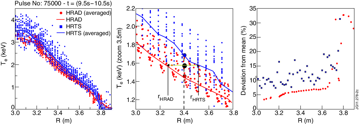
Figure 13: ECE TS radial discrepancies for typical JET plasma (JPN 75000, t=9.5-10.5s) for r=$3.5\text{\,}\mathrm{m}$. Plasma centre and separatrix are respectively at $\scriptstyle\sim$$3\text{\,}\mathrm{m}$ and $\scriptstyle\sim$$3.9\text{\,}\mathrm{m}$. Left: HRAD [red] and HRTS [blue] $\mathrm{T_{e}}$ profiles; data (points), average (lines). Centre: Deviations from time-average for each diagnostic. Right: estimation of ${r_{{\mathrm{\scriptscriptstyle HRAD}}}}-{r_{{\mathrm{\scriptscriptstyle HRTS}}}}$ for r=$3.5\text{\,}\mathrm{m}$

Observables for ECE TS radial discrepancies are designed in order to estimate the radial differences between HRAD and HRTS profiles. Fig. 13 shows how this estimation is done for r=$3.5\text{\,}\mathrm{m}$ for a typical JET pulse. The situation is the same with $\rho$ profiles. Plasma centre ($\rho\raise 0.73193pt\hbox{$\scriptstyle\sim$}0$) is usually missed by both diagnostics and the edge brings no additional information in ohmic and L-mode; the focus is then arbitrarily set to the gradient zone following median$\left({\rho_{{\mathrm{\scriptscriptstyle HRAD}}}}-{\rho_{{\mathrm{\scriptscriptstyle HRTS}}}},0.3<\rho<0.8\right)$.

The correction of the ECE TS radial discrepancies, and the various ways to do so, have been intensively discussed in the JET community for years. No definite answer has been found yet, because such corrections must ensure that HRAD and HRTS profiles match at the centre, in the gradient zone and at the plasma edge. Note that the situation worsens because the degree of the ECE TS mismatch is not always the same for ohmic, L- and H-mode plasmas.

In this part the possibility of a link between the ECE TS ratio (from MICH and LIDAR) and the ECE TS radial discrepancies (from HRTS and HRAD) is examined.

VII.2 Observations

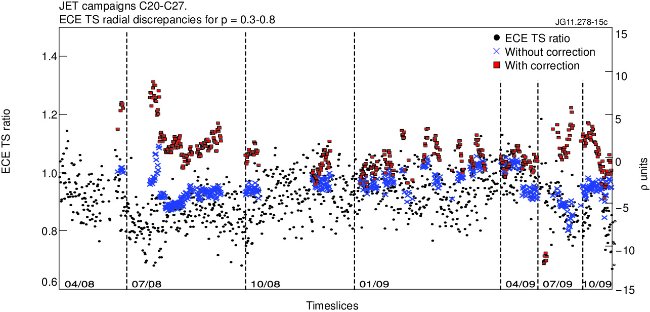
Figure 14: ECE TS ratio (left y-axis, black points) and ECE TS radial discrepancies median$\left({\rho_{{\mathrm{\scriptscriptstyle HRAD}}}}-{\rho_{{\mathrm{\scriptscriptstyle HRTS}}}},0.3<\rho<0.8\right)$ (right y-axis, $\rho$ units in $\%$) against timeslices for references pulses for C20-C27, where HRAD and HRTS data are available. Ohmic conditions, 147 pulses, 2878 timeslices. ECE TS radial discrepancies are non-corrected (cross, blue) and corrected (square, red) of the ECE TS ratio variations. Month/years are indicated by dashed lines.

Figure 15: Distribution of ECE TS radial discrepancies ($\rho$ units in $\%$), non-corrected (blue) and corrected (red) of the ECE TS ratio variations. Same pulses/timeslices selection as Fig. 14.

In Fig. 14, profiles mismatches are expressed as amplitude mismatches (ECE TS ratio, made of $\mathrm{\mathrm{T_{e}}_{\scriptscriptstyle MAX}}$ measurements from MICH and LIDAR) and radial ones (ECE TS radial discrepancies, averaged over $0.3<\rho<0.8$) for C20-C27 reference pulses where data from all these diagnostics is available. Only ohmic plasmas are analysed. Both quantities are well correlated. Radial discrepancies are mostly ranging from $-0.1$ to $0$ ($\rho$ units).

Correcting HRAD $\mathrm{T_{e}}$ profiles by increasing their values according to the ECE TS ratio, i.e. multiplying $\mathrm{\mathrm{T_{e}}_{\scriptscriptstyle HRAD}}$ by $\mathrm{\mathrm{T_{e}}_{\scriptscriptstyle MAX,{\textsc{\footnotesize LIDAR}}}}/\mathrm{\mathrm{T_{e}}_{\scriptscriptstyle MAX,{\textsc{\footnotesize MICH}}}}$, leads to a decrease of the ECE TS radial discrepancies to a -5% to 5% range (Fig. 14, with Fig. 15 for the distribution plot). This correction acts like a re-centring of the radial discrepancies around 0%; data dispersion is not reduced yet.

VII.3 Key points

ECE TS radial discrepancies might be explained as an amplitude shift following the ECE TS ratio – at least partially. Taking into account the variations of the ECE TS ratio is regarded as a first-step correction.

Cross-calibrations of HRTS and HRAD against MICH emphasises the role of MICH, as any possible drifts of MICH calibrations will appear on both ECE TS ratio and radial discreprancies sides. Possible drifts of LIDAR calibration appear only on the ratio side. Differences between corrected radial discrepancies and ratio variations are then mostly showing different behaviours between LIDAR central $\mathrm{T_{e}}$ and HRTS $\mathrm{T_{e}}$ in the gradient zone.

VIII Discussion & Consequences

VIII.1 Long-term stability of JET $\mathrm{T_{e}}$ measurement

As defined in (II), the $\mathrm{\mathrm{T_{e}}_{\scriptscriptstyle MAX}}$ quantity is a useful means of estimating the central electron temperature of JET plasmas and of comparing $\mathrm{T_{e}}$ measurements done by diagnostics with different lines of sight and/or diagnostics that do not always access the plasma centre.

This paper’s main finding is that the observed 15 years of central $\mathrm{T_{e}}$ measurements (1995-2009) featured in Fig. 3 and Fig. 4 mostly range between 0.5 and 1.25 (mean around 0.95) and exhibit non negligible variations through the years, with a 30% uncertainty observed on non-averaged ratio (see (III.3)). Large-scale structures and patterns are identified as large-scale temporal variations, amounting up to $\pm$20%. The complexity of the observed time drifts does not call for a simple explanation. Such variations are observed as well on more recent JET campaigns (C20-C27) in 2008 and 2009 (III.3.3).

No measurement for $\mathrm{T_{e}}$ could be used to assess the time stability of any of the studied diagnostics (III.3, III.4), even for the C20-C27 JET campaigns when four diagnostics were available – only three being calibrated in a way that their relative time variations are actually independent: MICH, LIDAR and HRTS. Analysis is therefore limited to relative variations between different measurements.

Following (III.4), variations of ECE TS ratio are disconnected from the 18 observed plasma parameters listed in Table 2 for carefuly selected reference pulses, apart from very low variations ($\pm$0.4%) of the magnetic field $\mathrm{B_{0}}$.

They appear yet to be quite satisfyingly correlated with the 12-month-period patterns shown by off-plasma KC1D integrator signals for the 2002-2009 time period (IV, Fig. 10). Those variations of KC1D integrator are believed to be caused by external or ambient temperature.

The analysis of the in-lab monitoring of MICH (V.1), consists of measurements against the same calibrated microwave source performed every few months since 1996, in order to check the long-term stability of the diagnostic. It is not possible to draw any firm conclusion on the link between drifts of ECE TS ratio and in-lab measurements performed on MICH, except that this monitoring shows that drifts of the ECE TS ratio cannot be explained only by the MICH drifts observed in-lab.

Regular calibrations of LIDAR are regularly performed: measurements of spectral functions and detector quantum efficiency are required to calculate plasma’s $\mathrm{T_{e}}$. Such calibrations have been done at random times of the year, since at least 15 years. These calibrations have always been very stable, so the authors would not expect any temperature dependance in them.

Off-plasma monitorings of both MICH and LIDAR do not show therefore any drifts that have been linked with the observed seasonal drifts of the ECE TS ratio.

For the 1995-2009 time period, JET $\mathrm{T_{e}}$ measured by ECE and TS diagnostics show large-scale slow-varying time-dependent variations up to $\pm$20%; calibrations drifts are suspected, and quite clear correlations are found with seasonal variations of the JET ambient temperature since mid-2002 and 2009.

The authors are not aware of such seasonal drifts between the ECE and TS systems installed and operated in any other large sized tokamak. As JET systems appear to suffer such sensitivity at an unexpected scale, it would be recommended to perform similar systematic checks on the electron temperature measurements on other large-sized tokamaks, if absolutely calibrated ECE and TS systems are available.

VIII.2 Revised uncertainty for overall measurement of JET electron temperature

As long as the cause(s) of the observed variations of ECE TS ratio remain(s) unknown, it should be considered as uncontrolled uncertainties affecting JET $\mathrm{T_{e}}$ measurements. The next paragraphs propose a revised uncertainty of JET $\mathrm{T_{e}}$ measurements from the experimental observations presented in this paper, i.e. the 1995-2009 time period. Future measurements are very likely to be similarly affected as well. It focuses on central $\mathrm{T_{e}}$; no better uncertainty is expected for non-central measurements.

Experimental uncertainty can be estimated to result from a systematic, non-time dependent uncertainty $\mathrm{(\delta T/T)_{cal}}$ accounting for absolute calibration and a time-dependent uncertainty $\mathrm{(\delta T/T)_{t}}$ caused by drifts, variations or just plain noise, following:

$$\mathrm{\delta T/T}\sim\sqrt{{\mathrm{(\delta T/T)_{cal}}}^{2}+{\mathrm{(\delta T/T)_{t}}}^{2}}$$

Estimated uncertainties of MICH and LIDAR calibrations i.e. $\mathrm{(\delta T/T)_{cal}}$ are within 5-10% (II.1). Experimental large-scale observations reported in this paper represent $\mathrm{(\delta T/T)_{t}}$ and are estimated at 15-20%, leading to the following estimation for the overall uncertainty for JET central $\mathrm{T_{e}}$ measurement:

$$\mathrm{\delta T/T}\sim 16-22\%$$

For non-central regions, issues specific to ECE radial localisation arise, reducing therefore the accuracy of MICH measurements. LIDAR measurements are not affected.

HRAD is cross-calibrated against MICH for each pulse, so $\mathrm{\mathrm{T_{e}}_{\scriptscriptstyle HRAD}}$ uncertainty can not be lower than MICH data in the plasma center. Same remark for non-central $\mathrm{T_{e}}$.

Absolute calibration of HRTS relies on HRAD for C20-C27, therefore, for this pulse range, it also relies on MICH. As long as no MICH-independent calibration is used, uncertainties of central and non-central $\mathrm{\mathrm{T_{e}}_{\scriptscriptstyle HRTS}}$ can not be lower then MICH uncertainties.

Possible drifts of HRTS calibration are not assessed in this paper, but it can be observed in Fig. 5 that variations of HRTS measurements for $\rho=0.5$ might be different to those of MICH or LIDAR. Conclusions for $\rho=0.2$ and 0.3 are similar. The uncertainty of HRTS data can not be estimated to be lower than the estimation for the three other diagnostics.

It is worth stressing that the confidence intervals resulting from absolute calibrations of MICH ($\pm{10}\%$) and LIDAR ($\pm{5}\%$) – see (II.1) – are clearly dwarfed by the time-dependent drifts observed, which are possibly caused by drifts of MICH and LIDAR calibrations.

VIII.3 Future work

Using MICH, LIDAR and HRTS as absolutely calibrated diagnostics, providing independent measurement of the same quantity ($\mathrm{T_{e}}$), it is hoped that enough data could be gathered, since C20 (April 2008), in order to discriminate which diagnostics suffer from calibration drifts. Few things can be done for the time period before 2008, where MICH and LIDAR were the only calibrated diagnostics.

For the next years of JET operation (2011 and after), the authors recommend a reference pulse to be designed and performed on a weekly basis at least for, say, 2 to 3 years. It is of course not possible to guarantee the perfect stability of the plasma parameters, but methodically repeating the same pulse will certainly help a lot to track the stability of the $\mathrm{T_{e}}$ measurements.

In parallel, in-lab monitoring of the diagnostics should be performed when possible. The frequency of the in-lab monitoring of MICH will be increased to a weekly or twice per month period. Ways of monitoring LIDAR and HRTS systems should be investigated.

IX Conclusion

Between 1995 and 2009, measurement of JET $\mathrm{T_{e}}$ has been carefuly reviewed using the two main diagnostics available for this time period: MICH (ECE), LIDAR (TS). The overall uncertainty of $\mathrm{T_{e}}$ measurements, based on these two diagnostics, is estimated to be as high as 16-22%, mostly made of large-scale time drifts.

From mid-2002 to 2009, the ratio of temperature measured by the two diagnostics (namely the ECE TS ratio) shows clear patterns with a 12-months period and a 15-20% amplitude. These drifts are regarded as calibration drifts, possibly caused by unexpected sensitivity to unknown parameters. External temperature on the JET site might is the best parameter suspected so far. The final cause of such variations has not been found, nor the way it affects MICH, LIDAR and/or (possibly) HRTS measurements.

It is not clear whether it is direct impact on one of the diagnostics or indirect via magnetics measurements, which have been shown to have seasonal drifts.

Solutions aiming at tracking down these unexpected uncertainties of JET $\mathrm{T_{e}}$ have been detailed and can be performed during the following JET campaigns (C28+, after October 2011), including reference pulses designed to be highly reproducible over time (new ITER-like wall permitting) and specific off-plasma monitoring of the diagnostics – when applicable.

Whatever causes these JET $\mathrm{T_{e}}$ drifts, this experimental issue is regarded as crucial for data quality. Long-term observed ECE TS radial discrepancies have been shown to be linked to these seasonal drifts. Tackling this issue and elucidating the cause of these unexplained seasonal variations is of great importance, impacting to the quality of JET $\mathrm{T_{e}}$ measurements.

This work was supported by EURATOM and carried out within the framework of the European Fusion Development Agreement. The views and opinions expressed herein do not necessarily reflect those of the European Commission.

References

- Baker et al. (1984) Baker, E., Bartlett, D., Campbell, D. J., Costley, A., and Hubbard, A.E. Moss, D., in Proceedings of the \nth4 Joint Workshop on ECE and ECRH, New York (Oxford University, 1984).
- Barrera, de la Luna, and Contributors (2008) Barrera, L., de la Luna, E., and Contributors, L. F. J. E. (JET EFDA Contributors), AIP Conference Proceedings 988, 123 (2008).
- Bartlett (1992) Bartlett, D., in Proceedings of the \nth8 International Workshop on ECE and ECRH, Gut Ising, Germany (Oxford University, 1992).
- Bartlett et al. (1987) Bartlett, D., Campbell, D. J., Costley, A., Kissel, S., Lopez Cardozo, N., Gowers, C. W., Nowak, S., Oyevaar, T., Salmon, N. A., and Tubbing, B. J., in Proceedings of the \nth6 Joint Workshop on ECE and ECRH, New York (Oxford University, 1987).
- Bekefi (1966) Bekefi, G., Radiation processes in plasmas, Wiley series in plasma physics (Wiley, 1966).
- Costley et al. (1984) Costley, A., Baker, E., Bartlett, D., Campbell, D. J., Kiff, M., and Neill, G., in Proceedings of the \nth4 Joint Workshop on ECE and ECRH, New York (Oxford University, 1984).
- Costley et al. (1974) Costley, A. E., Hastie, R. J., Paul, J. W. M., and Chamberlain, J., Phys. Rev. Lett. 33, 758 (1974).
- Eriksson and Hellsten (1995) Eriksson, L.-G. and Hellsten, T., Physica Scripta 52, 70 (1995).
- Eriksson, Hellsten, and Willen (1993) Eriksson, L.-G., Hellsten, T., and Willen, U., Nuclear Fusion 33, 1037 (1993).
- Flanagan et al. (2010) Flanagan, J., Balboa, I., Beurskens, M., Kempenaars, M., Maslov, M. Alfier, A., Pasqualotto, R., and contributors, J. E., in \nth37 Institute of Physics Plasma Conference, Winderemere, Lake District, Cumbria, 2010 (2010).
- Garbet et al. (1992) Garbet, X., Payan, J., Laviron, C., Devynck, P., Saha, S., Capes, H., Chen, X., Coulon, J., Gil, C., Harris, G., Hutter, T., Pecquet, A.-L., Truc, A., Hennequin, P., Gervais, F., and Quemeneur, A., Nuclear Fusion 32, 2147 (1992).
- Gowers et al. (1995) Gowers, C. W., Brown, B. W., Fajemirokun, H., Nielsen, P., Nizienko, Y., and Schunke, B., Review of Scientific Instruments 66 (1995), 10.1063/1.1146321.
- Horton (2005) Horton, A., JET internal report (2005).
- Hutchinson (2002) Hutchinson, I., Principles of plasma diagnostics (Cambridge University Press, 2002).
- Lao et al. (1985) Lao, L., John, H. S., Stambaugh, R., and Pfeiffer, W., Nuclear Fusion 25, 1421 (1985).
- de la Luna et al. (2003) de la Luna, E., Krivenski, V., Giruzzi, G., Gowers, C., Prentice, R., Travere, J. M., and Zerbini, M., Review of Scientific Instruments 74, 1414 (2003).
- de la Luna et al. (2004) de la Luna, E., Sanchez, J., Tribaldos, V., Conway, G., Suttrop, W., Fessey, J., Prentice, R., Gowers, C., and Chareau, J. M, J.-E. c., Review of Scientific Instruments 75, 3831 (2004).
- Murari et al. (2011) Murari, A., Mazon, D., Gelfusa, M., Folschette, M., Quilichini, T., and Contributors, J.-E., Nuclear Fusion 51, 053012 (2011).
- O’Brien et al. (1992) O’Brien, D., Lao, L., Solano, E., Garribba, M., Taylor, T., Cordey, J., and Ellis, J., Nuclear Fusion 32, 1351 (1992).
- Pasqualotto et al. (2004) Pasqualotto, R., Nielsen, P., Gowers, C., Beurskens, M., Kempenaars, M., Carlstrom, T., and Johnson, D., Review of Scientific Instruments 75, 3891 (2004), iSI Document Delivery No.: 866EFPart 2.
- Salmon (1987) Salmon, N. A. e. a., in Proceedings of the \nth6 Joint Workshop on ECE and ECRH, New York (Oxford University, 1987).
- Schmuck (2011) Schmuck, S., in EFDA/JET DVCM presentation (2011).
- Schmuck et al. (2012) Schmuck, S., Fessey, J., Gerbaud, T., Alper, B., Beurskens, M., Figini, L., de la Luna, E., Sirinelli, A., and Contributors, J. E., Review of Scientific Instruments (to be published) (2012).
- Von Hellermann and Summers (1993) Von Hellermann, M. and Summers, H., Atomic and Plasma Material Interaction Processes in Controlled Thermonuclear Fusion (1993).
- Wesson and Campbell (1997) Wesson, J. and Campbell, D., Tokamaks, Oxford engineering science series (Clarendon Press, 1997).
- Zerbini (2007) Zerbini, M., in EFDA/JET DVCM presentation (2007).
- Zerbini et al. (2003) Zerbini, M., Chareau, J. M., Mazon, D., Riva, M., Felton, R., Joffrin, E., Lennholm, M., and Prentice, R., in Electron Cyclotron Emission and Electron Cyclotron Heating (2003) pp. 227–232.