Quantum quenches in one-dimensional gapless systems

Abstract

We present a comparison between the bosonization results for quantum quenches and exact diagonalizations in microscopic models of interacting spinless fermions in a one-dimensional lattice. The numerical analysis of the long-time averages shows that density-density correlations at small momenta tend to a non-zero limit, mimicking a thermal behavior. These results are at variance with the bosonization approach, which predicts the presence of long-wavelength critical properties in the long-time evolution. By contrast, the numerical results for finite momenta suggest that the singularities at $2k_{F}$ in the density-density correlations and at $k_{F}$ in the momentum distribution are preserved during the time evolution. The presence of an interaction term that breaks integrability flattens out all singularities, suggesting that the time evolution of one-dimensional lattice models after a quantum quench may differ from that of the Luttinger model.

1 Introduction

The study of non-equilibrium dynamics of isolated many-body quantum systems has been triggered by the recent progress in ultra-cold gases experiments greiner2002 ; kinoshita2006 ; hofferberth2007 ; trotzky2011 . In fact, these systems are sufficiently weakly coupled to the external environment and, therefore, the observation of essentially unitary non-equilibrium time evolution on long time scales is possible. The availability of experimental controllable systems, whose properties can be accurately described by simple models, provides an unprecedented opportunity to explore new frontiers in physics, including non-equilibrium dynamics in closed interacting quantum systems polkovnikov2011 . The experimental advances posed serious challenges to the theory and new paradigms must be developed. Although we achieved a satisfactory understanding of correlated materials at equilibrium, the basic principles governing quantum systems far from equilibrium are still in their infancy.

A common protocol to study out-of-equilibrium problems is called quantum quench and consists in preparing the system in the ground state of a given Hamiltonian and then suddenly let it evolve under the action of a new Hamiltonian. Since the evolution is unitary, the energy stored into the initial state is conserved during the dynamics. The interest in these classes of non-equilibrium problems relies on both the dynamics itself barmettler2009 and the long-time properties, including the highly debated issue of thermalization rigol2008 . Quantum quenches have been the subject of vast literature focusing on different systems polkovnikov2011 . In particular, one-dimensional (1D) models have been largely explored cazalilla2011 . From the theoretical point of view, there are many different analytical or numerical methods that may give useful insights into the dynamical properties and the nature of the steady state (if any), inquiring the possibility to reach thermalization cazalilla2006 ; kollath2007 ; manmana2007 ; calabrese2011 . Integrable models require a separate analysis integrability , because a complete thermalization is not expected, due to the existence of a extensive number of conserved quantities. In this regard, it has been suggested that the steady state of an integrable system of hard-core bosons may be described by a generalized Gibbs ensemble (GGE) that maximizes the entropy with all possible constraints imposed by the existence of (infinite) integrals of motion rigol2007 .

At the roots of many-body theory in condensed matter theory, the Luttinger model was introduced to describe a system of interacting fermions in 1D; the approximation of considering fully linear dispersions made it possible an exact solution in terms of bosonic variables, e.g., fermionic densities luttinger1963 ; lieb1965 (hence the name bosonization). Later, the asymptotic forms of one- and two-particle correlations in equilibrium were obtained by Luther and Peschel luther1974 and Haldane haldane1980 ; haldane1981 proposed that this model may generically describe the low-energy properties of a broad class of systems in 1D, now known as Tomonaga-Luttinger (TL) liquids giamarchi2004 .

Recently, the bosonization approach for the Luttinger model has been used to compute the time evolution after a quantum quench cazalilla2006 . According to these results, real space correlation functions evolve towards a steady state. Remarkably, the spatial decay of correlations is always governed by critical exponents, which however are different from the ground state ones. On the other hand, generic quantum models in 1D are expected to give rise to thermalization, where all singularities are washed out. It is therefore important to test the bosonization results against numerical simulations of lattice models in order to better understand the non-equilibrium dynamics of quantum one-dimensional models. Recently, a numerical investigation of a one-dimensional lattice model of spinless fermions has been performed by using density-matrix renormalization group technique karrasch2012 . The analysis of the short-time evolution of few observables suggests that the bosonization predictions are indeed verified also in lattice models. By contrast, a renormalization-group approach of the bosonized Hamiltonian in presence of a periodic potential has suggested that temperature effects and dissipation among bosonic modes may be generated, removing all singularities mitra2011 . In this paper, we aim at performing a detailed comparison between the TL approach and exact calculations (by Lanczos diagonalizations) on a microscopic model of interacting fermions on a 1D lattice. Although the latter approach is limited to relatively small system sizes, we obtain a clear and unambiguous evidence that a TL analysis misses important aspects of the long-time behavior.

The paper is organized as follow: in sections 2 and 3, we review the basic steps of the bosonization technique and the results for the time-dependent correlation functions; in section 4, we present the lattice models and the numerical method based upon Lanczos diagonalization; in section 5, we make some preliminary considerations on time evolution on finite sizes and time averages; in section 6, we show the results; in section 7, we draw our conclusions. Finally, in the appendix A, we show that the exact time evolution of the TL model can be described by a density-density Jastrow wave function.

2 Bosonization

The TL model is obtained from a generic Hamiltonian of interacting spinless fermions in a 1D lattice:

$${\cal H} = {\cal H}_{0}+{\cal H}_{\rm int},$$ (1)

$${\cal H}_{0} = \sum_{k}\xi_{k}c^{\dagger}_{k}c_{k},$$ (2)

$${\cal H}_{\rm int} = \frac{1}{2L}\sum_{k,k^{\prime},q\neq 0}V(q)c^{\dagger}_{k}c^{\dagger}_{k^{\prime}}c_{k^{\prime}-q}c_{k+q},$$ (3)

where $\xi_{k}$ represents the fermionic dispersion and $L$ is the size of the lattice. The specific form of the interaction $V(q)$ depends upon the details of the model. In general, it is assumed that well defined values for the forward scattering (small $q$’s) and backscattering ($q\approx\pm 2k_{F}$) are given. The basic idea is to linearize the dispersion relation $\xi_{k}$ near the Fermi energy, i.e., $\xi_{k}\approx v_{F}(|k|-k_{F})$. It is convenient to assume that this linear dispersion extends for all $k\in[-\infty,\infty]$. In this case, the particle belonging to either branch, denoted by left or right, are distinguishable and will be considered as two different species of fermions (Luttinger model). luttinger1963

The Hamiltonian (1) can be written in terms of two density operators (for left and right particles):

$$\rho_{L}(q)=\sum_{k<0}c_{k}^{\dagger}c_{k+q}\;\;\;\;\;\rho_{R}(q)=\sum_{k>0}c_{k}^{\dagger}c_{k+q}.$$ (4)

Indeed, up to a constant, we obtain:

$${\cal H}_{0} = \frac{2\pi v_{F}}{L}\sum_{q>0}\left[\rho_{R}(q)\rho_{R}(-q)+\rho_{L}(q)\rho_{L}(-q)\right],$$ (5)

$${\cal H}_{\rm int} = \frac{V}{2L}\sum_{q>0}\left[\rho_{R}(q)+\rho_{L}(q)\right]\left[\rho_{R}(-q)+\rho_{L}(-q)\right],$$ (6)

where $V=V(0)-V(2k_{F})$. In the standard approach for bosonization, new boson operators are considered:

$$a_{q} = \sqrt{\frac{2\pi}{qL}}\rho_{R}(q)\;\;\;\;\;a_{q}^{\dagger}=\sqrt{\frac{2\pi}{qL}}\rho_{R}(-q),$$ (7)

$$b_{q} = \sqrt{\frac{2\pi}{qL}}\rho_{L}(-q)\;\;\;\;\;b_{q}^{\dagger}=\sqrt{\frac{2\pi}{qL}}\rho_{L}(q),$$ (8)

such that $a$ and $b$ obey to the usual canonical bosonic commutation relations. In terms of these operators the Hamiltonian becomes:

$${\cal H}_{0} = v_{F}\sum_{q>0}q\left(a_{q}^{\dagger}a_{q}+b_{q}^{\dagger}b_{q}\right)$$ (9)

$${\cal H}_{\rm int} = \frac{V}{2\pi}\sum_{q>0}q\left(a_{q}^{\dagger}a_{q}+b_{q}^{\dagger}b_{q}+a_{q}b_{q}+b_{q}^{\dagger}a_{q}^{\dagger}\right).$$ (10)

Therefore, the full Hamiltonian may be easily diagonalized by using a $q$-independent Bogoliubov transformation:

$$\alpha_{q} = ua_{q}+vb_{q}^{\dagger},$$ (11)

$$\beta_{q} = va_{q}^{\dagger}+ub_{q},$$ (12)

with $u^{2}-v^{2}=1$; therefore, we can take $u=\cosh\phi$ and $v=\sinh\phi$, with $\tanh(2\phi)=V/(2\pi v_{F}+V)$. We mention that $u$ and $v$ can be expressed in terms of the standard Luttinger parameter $K$, namely $u=(1+K)/(2\sqrt{K})$ and $v=(1-K)/(2\sqrt{K})$, with $K=(u-v)^{2}=\cosh 2\phi-\sinh 2\phi$.

After the Bogoliubov transformation, the TL Hamiltonian becomes

$${\cal H}=\sum_{q>0}\epsilon_{q}\left(\alpha_{q}^{\dagger}\alpha_{q}+\beta_{q}^{\dagger}\beta_{q}\right),$$ (13)

where:

$$\epsilon_{q}=\left\{\sqrt{v_{F}^{2}+\frac{v_{F}V}{\pi}}\right\}q=c_{s}q$$ (14)

is the excitation energy for the $q$-mode.

Finally, let us indicate by $|0\rangle_{ab}$ and $|0\rangle_{\alpha\beta}$ the vacuum states of $(a,b)$ and $(\alpha,\beta)$ bosons, which coincide with the ground states for the non-interacting [Eq. (9)] and the interacting [Eq. (13)] systems, respectively. Then, the ground state of the full Hamiltonian can be written as:

$$|0\rangle_{\alpha\beta}\propto\exp{\left[-\frac{v}{u}\sum_{q>0}\alpha_{q}^{\dagger}\beta_{q}^{\dagger}\right]}|0\rangle_{ab}.$$ (15)

Let us now consider the time evolution of the non-interacting state $|0\rangle_{ab}$ by using the interacting Hamiltonian ${\cal H}$, corresponding to a quantum quench from $V=0$ to a finite value of the interaction strength. Interestingly, the time evolution has a very simple and instructive form, which will be used in the following Section. Indeed, from Eq. (15) we can write

$$|0\rangle_{ab}\propto\exp{\left[\frac{v}{u}\sum_{q>0}\alpha_{q}^{\dagger}\beta_{q}^{\dagger}\right]}|0\rangle_{\alpha\beta},$$ (16)

and therefore

$$e^{-i{\cal H}t}|0\rangle_{ab}\propto\exp{\left[\frac{v}{u}\sum_{q>0}e^{-2i\epsilon_{q}t}\alpha_{q}^{\dagger}\beta_{q}^{\dagger}\right]}|0\rangle_{\alpha\beta}$$

$$\propto\exp{\left[\frac{v}{u}\sum_{q>0}\left(e^{-2i\epsilon_{q}t}-1\right)\alpha_{q}^{\dagger}\beta_{q}^{\dagger}\right]}|0\rangle_{ab}$$ (17)

In appendix A, we show that both the exact ground state (15) and the time evolution of Eq. (17) may be rewritten in term of density-density Jastrow wave functions, jastrow1955 which are commonly used to describe ground-state properties of correlated systems, capello2005 ; capello2007 and more recently also out of equilibrium dynamics. carleo2012

3 Correlation functions

Here, we give a brief overview of the time-dependent correlation functions; our results agree with those of Ref. cazalilla2006 for the Luttinger model. Let us suppose that at $t=0$ the system is set in the non-interacting ground state $|0\rangle_{ab}$, while for $t>0$ it evolves according to the interacting Hamiltonian ${\cal H}$:

$$|\Phi(t)\rangle=e^{-i{\cal H}t}|0\rangle_{ab}.$$ (18)

Then, the bosonization technique allows one to directly compute the density-density correlation function:

$$N_{q}(t)=\frac{1}{L}\langle\Phi(t)|n_{q}n_{-q}|\Phi(t)\rangle,$$ (19)

where $n_{\pm q}=\rho(\pm q)=\rho_{L}(\pm q)+\rho_{R}(\pm q)$. Indeed, by using Eqs. (7), (8), (11), (12) and (17), after some straightforward algebra, we obtain the simple expression:

$$N_{q}(t)=\frac{q}{2\pi}\left[A+B\cos(2\epsilon_{q}\;t)\right].$$ (20)

where

$$A = (u^{2}+v^{2})(u-v)^{2}=\frac{1+K^{2}}{2},$$ (21)

$$B = 1-A.$$ (22)

This result shows that $N_{q}(t)$ does not relax to a finite limit but instead oscillates with a single frequency that equals twice the value of the excitation energy $\epsilon_{q}=c_{s}q$. By performing a Fourier transform (that takes into account an ultraviolet cutoff), it is possible to obtain the $q\sim 0$ (spatially monotonic) contribution of the density-density correlations:

$$N_{r}(t)=n^{2}-\frac{1}{4\pi^{2}}\Bigg{[}\frac{2A}{r^{2}}+\frac{B}{(r+2c_{s}t)^{2}}+\frac{B}{(r-2c_{s}t)^{2}}\Bigg{]},$$ (23)

which shows that, for each fixed distance $r$, $\lim_{t\to\infty}N_{r}(t)$ converges to a finite value. Notice that the asymptotic behavior of $N_{r}(t)$ coincides with the Fourier transform of the time average of $N_{q}(t)$, which equals $Aq/{2\pi}$ and differs from the known ground state behavior $Kq/{2\pi}$.

For completeness, we also report the time evolution of the $q\sim 2k_{F}$ singular contribution to the density correlations:

$$N_{r}(t)\propto\left(\frac{4c_{s}^{2}t^{2}}{|r^{2}-4c_{s}^{2}t^{2}|}\right)^{2uv(u-v)^{2}}\frac{\cos(2k_{F}r)}{r^{2(u^{2}+v^{2})(u-v)^{2}}},$$ (24)

and the $q\sim k_{F}$ singularity of the one-body density matrix:

$$\langle\Phi(t)|c_{r}^{\dagger}c_{0}|\Phi(t)\rangle\propto\left(\frac{|r^{2}-4c_{s}^{2}t^{2}|}{4c_{s}^{2}t^{2}}\right)^{2u^{2}v^{2}}\frac{\cos(k_{F}r)}{r^{1+4u^{2}v^{2}}}.$$ (25)

At fixed $r$, for $t\to\infty$ the first factor in these expressions tends to unity, showing that the correlation functions in real space tend again to a finite limit for large times.

4 Models and numerical methods

Let us now define the microscopic model that will be used to make comparisons with the bosonization predictions: a system of spinless fermions interacting via a repulsive short-range potential:

$${\cal H}=-J\sum_{\langle i,j\rangle}c^{\dagger}_{i}c_{j}+H.c.+V\sum_{\langle i,j\rangle}n_{i}n_{j}+V^{\prime}\sum_{\langle\langle i,j\rangle\rangle}n_{i}n_{j}$$ (26)

where $\langle i,j\rangle$ and $\langle\langle i,j\rangle\rangle$ indicate nearest-neighbor and next-nearest-neighbor sites, respectively. $c^{\dagger}_{i}$ ($c_{i}$) creates (destroys) a fermion on the site $i$, and $n_{i}=c^{\dagger}_{i}c_{i}$ is the fermion density. The number of sites and fermions are denoted by $L$ and $N$, respectively, so that the fermion density is $n=N/L$. Periodic or antiperiodic boundary conditions are considered for odd or even $N$, respectively. In the following, we take $J=1$, as energy scale. Most of the calculations are done in presence of nearest-neighbor interaction $V$ only (which corresponds to an integrable system), similar results are also obtained including a finite next-nearest-neighbor $V^{\prime}$ (that breaks the integrability). Notice that the system we investigate is equivalent to a model of hard-core bosons with Hamiltonian (26) and periodic boundary conditions.

The quantum quench consists in taking an initial wave function $|\Psi(0)\rangle$, which is the ground state of Eq. (26) with $V=V_{i}$ (and $V^{\prime}=V^{\prime}_{i}$), and letting it evolve under the same Hamiltonian with $V=V_{f}$ (and $V^{\prime}=V^{\prime}_{f}$). By using the Lanczos method, it is possible to perform the exact time evolution of any initial state. Indeed, the full time interval can be split in small steps $\Delta t$ and the time evolution can be evaluated recursively:

$$|\Psi(t+\Delta t)\rangle=e^{-i{\cal H}\Delta t}|\Psi(t)\rangle.$$ (27)

Each small-time evolution can be computed by a truncated Taylor expansion:

$$|\Psi(t+\Delta t)\rangle\simeq\sum_{k=0}^{k_{c}}\frac{(-i\Delta t)^{k}}{k!}{\cal H}^{k}|\Psi(t)\rangle,$$ (28)

where the cut-off $k_{c}$ is chosen as to preserve energy conservation to the desired numerical accuracy.

5 Preliminary considerations

From what we have described in the previous section, by using the Lanczos technique, it is in principle possible to compute the time-evolution of any observable:

$${\cal O}(t)=\langle\Psi(t)|{\cal O}|\Psi(t)\rangle.$$ (29)

However, we must emphasize that, on finite systems, recurrence effects are always present and, at long times, the dynamics suffers from size effects. Indeed, the initial state inevitably contains excitations that, under the time evolution, may “travel” all along the chain. In models where the full spectrum is described by non-interacting quasi-particles, interference effects appear after the time $T\simeq L/v$, where $v$ is the velocity of the elementary excitations. However, for generic models, this recurrence time may be much larger and relies on the energy differences of the (finite-size) many-body spectrum. Nevertheless, although for large times ${\cal O}(t)$ may suffer from size effects, its average over long times is fully meaningful. In order to give some support on this claim, we consider a case where exact results can be obtained in the thermodynamic limit. In particular, we consider the case where the density of spinless fermions is half filled (i.e., $n=1/2$) and the initial state has a fermion every two sites, i.e., $|\Psi(0)\rangle\equiv|\dots,1,0,1,0,1,0,\dots\rangle$. Then, the time evolution is done by the Hamiltonian (26) with $V=V^{\prime}=0$. In this case, density-density correlation functions

$$N_{r}(t)=\langle\Psi(t)|n_{r}n_{0}|\Psi(t)\rangle-\langle\Psi(t)|n_{r}|\Psi(t)\rangle\langle\Psi(t)|n_{0}|\Psi(t)\rangle$$ (30)

can be computed analytically directly in the thermodynamic limit. This correlation function is translationally invariant and its Fourier transform is given by:

$$N_{q}(t)=\frac{1}{4}\left[1-J_{0}(8t\sin(q/2))\right],$$ (31)

where $J_{0}(x)$ is the Bessel function of order zero. In Fig. 1, we compare Eq. (31) with the case of $L=32$ for $q=\pi/16$. Although the results for $L=32$ clearly deviate from the analytical ones for $t\gtrsim 35$, their time average is fully meaningful and gives an excellent approximation of the exact outcome. Therefore, in the following we will consider time averages over relatively large times (up to $t=100$) to obtain an estimation of the long-time behavior.

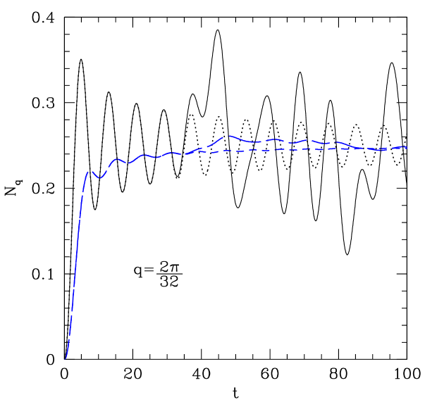
Figure 1: (Color online) Time evolution of the density-density correlation $N_{q}(t)$ of the inhomogeneous state $|\dots,1,0,1,0,1,0,\dots\rangle$ that is evolved with the non-interacting Hamiltonian of Eq. (26). Results with $L=32$ (solid black curve) are compared with the thermodynamic limit (dotted black curve). The time averages are also reported (blue dashed lines).

6 Numerical results

We begin by considering the case of $V^{\prime}=0$. In this case, the low-energy properties of Eq. (26) are well described by a (gapless) TL liquid, except for $n=1/2$ and $V>2$, where a (gapped) charge-density-wave insulator is obtained. giamarchi2004 Since we want to compare the numerical calculations with the TL theory, in the following, we take $n=1/4$ (similar results have been also obtained with other densities, e.g., $n=1/3$). We will show the case of $V_{i}=0$ (and $V^{\prime}_{i}=0$), so that the initial wave function corresponds to the case of free spinless fermions. However, we checked that qualitatively similar results are obtained also for finite $V_{i}>0$.

Some initial information about the time evolution can be obtained from the analysis of the overlaps between the initial wave function $|\Psi(0)\rangle$ and the eigenstates of the evolving Hamiltonian $|\Phi_{n}\rangle$ (with ${\cal H}|\Phi_{n}\rangle=E_{n}|\Phi_{n}\rangle$) i.e., $c_{n}=\langle\Phi_{n}|\Psi(0)\rangle$. Indeed, these coefficients play an important role in the time evolution of a generic observable ${\cal O}$:

$$\langle\Psi(t)|{\cal O}|\Psi(t)\rangle=\sum_{n,n^{\prime}}e^{-i(E_{n}-E_{n^{\prime}})t}c_{n^{\prime}}^{*}c_{n}\langle\Phi_{n^{\prime}}|{\cal O}|\Phi_{n}\rangle.$$ (32)

This expression shows that the temporal evolution of ${\cal O}$ contains all the frequencies $\omega=E_{n}-E_{n^{\prime}}$ corresponding to the gaps in the excitation spectrum of the interacting system. Bosonization predicts a linear excitation spectrum at low energies that, in the special case of the observable $N_{q}$ written in terms of density operators, gives rise to a single frequency oscillatory behavior with $\omega=2\epsilon_{q}$, see Eq. (20). The excitation spectrum of a lattice model is considerably more complex and curvature effects are expected to introduce further frequencies in the power spectrum of the time evolution of ${\cal O}$. Pure oscillatory behavior would correspond to a $c_{n}$ distribution peaked in a small energy interval $E_{n}-E_{n^{\prime}}$ and to matrix elements $\langle\Phi_{n^{\prime}}|{\cal O}|\Phi_{n}\rangle$ able to connect a single pair of excitations.

In Fig. 2, we show the results for $P(E)$ in two different cases with $V_{f}=3$ and $10$, which will be considered in the following discussion. The $c_{n}$ distribution is indeed confined in a limited energy interval although a significant additional peak at high energy appears for strong interactions.

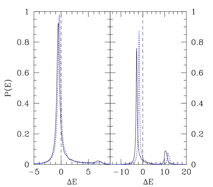
Figure 2: (Color online) Distribution $P(E)$ of the overlaps (squared) between the initial wave function and the eigenstates of the evolving Hamiltonian as a function of the energy of the eigenstates $E$. Energies have been shifted, namely $\Delta E=E-E_{i}$ (where $E_{i}$ is the energy stored into the initial state), so that $\Delta E=0$ corresponds to the average value of the distribution. Lattice sizes are $L=20$ (dashed line) and $L=32$ (solid line). A broadening of the finite size $\delta$-like peaks has been introduced. The value of the interaction strength is $V=3$ (left panel) and $V=10$ (right panel).

Let us now move to the main part of the paper and consider the density-density correlations:

$$N_{q}(t)=\frac{1}{L}\sum_{i,j}e^{iq(R_{i}-R_{j})}\langle\Psi(t)|n_{i}n_{j}|\Psi(t)\rangle.$$ (33)

To compare the exact diagonalizations with bosonization results of Eq. (20), we have to compute the parameters $A$ and $B$, together with the renormalized fermionic dispersion $\epsilon_{q}=c_{s}q$. This can be easily done by calculating the Luttinger parameter $K$ and the velocity $c_{s}$, which can be obtained either by Bethe Ansatz (for $V^{\prime}=0$) or numerically (for $V^{\prime}\neq 0$). giamarchi2004

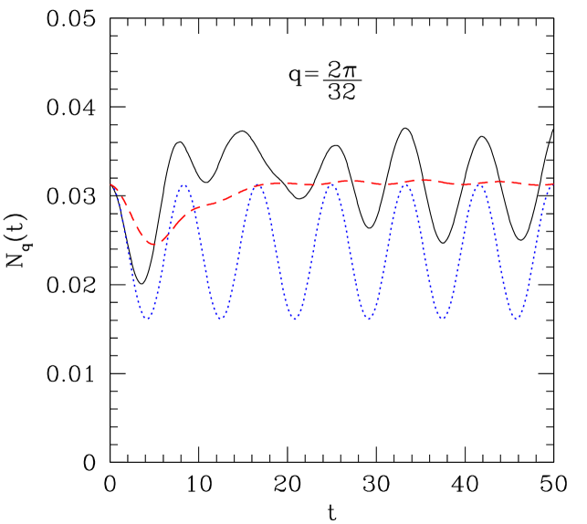
Figure 3: (Color online) Time evolution of the density-density correlation $N_{q}(t)$ at quarter filling for a quench from $V_{i}=0$ to $V_{f}=3$ and $q=2\pi/32$ (the system size is $L=32$). The time average (dashed line) and the bosonization results (dotted line) are also shown.

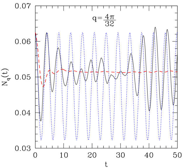
Figure 4: (Color online) Same as in Fig. 3 for $q=4\pi/32$.

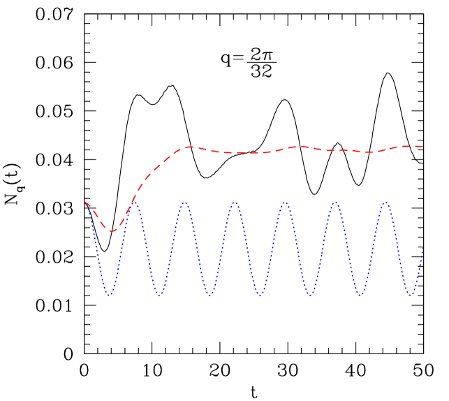
Figure 5: (Color online) Same as in Fig. 3 for $V_{f}=10$.

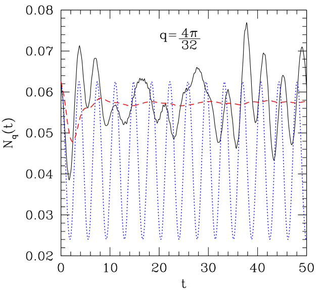
Figure 6: (Color online) Same as in Fig.5 for $q=4\pi/32$.

In Figs. 3, 4, 5, and 6, we report the results for $V_{f}=3$ and $10$ and the two smallest non-zero momenta on the 32-site lattice, namely $q=2\pi/32$ and $4\pi/32$, together with the bosonization prediction of Eq. (20). The time average of the oscillating signal stabilizes at a well defined value for sufficiently large times, a feature also shared with the bosonization approach. Nevertheless, long-time averages in the TL model are always different from those obtained in the lattice model, where the signal shows significant deviations from periodicity, as a consequence of the coupling among excitation modes. However, for small quenches (e.g., $V_{f}=3$) and small momenta (e.g., $q=2\pi/32$), after an initial transient, a stable oscillatory behavior dominated by a single frequency is observed. In this case, the observed frequency agrees very well with the TL predictions. For larger values of the momenta and for larger quenches, the signal acquires a more complex periodicity.

We remark that both the amplitude and the average value of the numerical results considerably differ from the bosonization predictions. The discrepancy increases for larger quenches, where, even for the smallest momenta available in the Lanczos diagonalizations, the dynamical signal contains more than one frequency and the TL predictions become less and less accurate. For example, for $V_{f}=10$ and $q=2\pi/32$, the lattice model shows at least two relevant frequencies (see Fig. 5), the largest one being very close to the TL result. Also the discrepancy between the average values grows when increasing the final value of the interaction strength.

Although the signal may have a very strong dependence on the system size for large times, the average value is quite stable, showing that the long-time properties may be safely extracted from our finite-size calculations, see Fig. 7. Moreover, there is some evidence that fluctuations around the average value decrease by increasing the cluster size, suggesting the possibility that in the thermodynamic limit (and long times) the signal experiences a complete damping towards its average value.

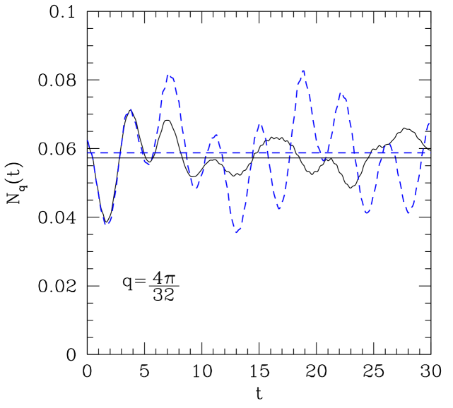
Figure 7: (Color online) Time evolution of the density-density correlation $N_{q}(t)$ at quarter filling for a quench from $V_{i}=0$ to $V_{f}=3$ and $q=2\pi/32$ for $L=16$ (dashed lines) and $L=32$ (solid lines). The two averages, evaluated after a long time interval (i.e., $t=100$), are also reported (horizontal lines).

From these results, it is clear that bosonization misses relevant aspects of the dynamics after a quantum quench. More surprisingly, the long-time average of the density-density correlations are qualitatively different from the bosonization predictions for $q\to 0$. Indeed, in the TL theory, a linear behavior ${\overline{N}}_{q}=A/(2\pi)q$ (where the overbar indicates the long-time average) is found from Eq. (20), while, the numerical results clearly indicate a finite limit ${\overline{N}}_{q}={\rm const}$ as $q\to 0$, see Figs. 8 and 9. The slope of ${\overline{N}}_{q}$ predicted by bosonization is also shown in the figures and remarkably describes the behavior of correlations in an intermediate range of wave-vectors. It appears that although the TL model does not capture an important qualitative feature of the long wave-length behavior of correlations, it is still able to correctly reproduce the physics of the asymptotic state when the size of the system is not exceedingly large. We will see that similar features also appear in other observables, like the momentum distribution.

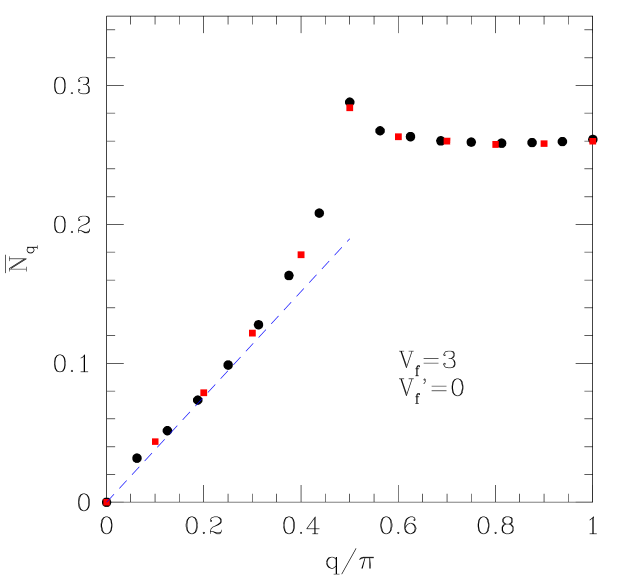
Figure 8: (Color online) Time average of density-density correlation $N_{q}(t)$ for a quench from $V_{i}=0$ to $V_{f}=3$ for $L=20$ (squares) and $L=32$ (circles). The dashed line shows the behavior expected from bosonization at small momenta.

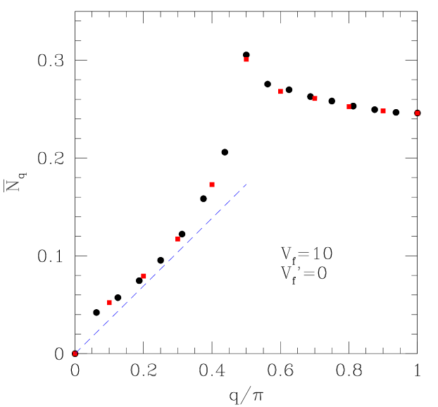
Figure 9: (Color online) Same as in Fig. 8 for $V_{f}=10$.

Although Lanczos diagonalizations are performed on finite lattices, these conclusions are robust against finite-size effects, as proved by the nice collapse of the numerical data on $L=20$ and $32$ clusters, see Figs. 8 and 9. On the one hand, a non-vanishing long-wavelength limit of ${\overline{N}}_{q}$ is reminiscent of a finite temperature behavior, where singularities are washed out by thermal fluctuations. notethermalization On the other hand, our finite-size calculations provide some evidence for the existence of a cusp at $q=2k_{F}$. Unfortunately, due to the intrinsic statistical error induced by the time average procedure, the (critical) exponent related to the $q=2k_{F}$ singularity cannot be accurately determined from Lanczos data. The possibility that the cusps are eventually rounded in the thermodynamic limit cannot be ruled out either. In any case, we find that ${\overline{N}}_{q}$ cannot be suitably fitted by using a single effective temperature (as expected, since the model is integrable).

The failure of the bosonization approach may be due to the presence of a perfectly linear fermionic dispersion (up to infinity or to a given cutoff) in the TL model. While this approximation is known to give the correct low-energy behavior for static properties, affleck1989 ; sorella1990 it breaks down when considering the real time evolution for long times, where the initial state may contain high-energy excitations, not adequately represented within the TL model. Moreover, bosonization describes uncoupled modes, which do not interact and, therefore, does not include the effects due to dephasing. In this regard, band curvature and finite bandwidth effects are expected to play a crucial role beyond the simple TL results.

Let us now consider the momentum distribution:

$$n_{k}(t)=\frac{1}{L}\sum_{i,j}e^{ik(R_{i}-R_{j})}\langle\Psi(t)|c^{\dagger}_{i}c_{j}|\Psi(t)\rangle.$$ (34)

The numerical results for the time average ${\overline{n}}_{k}$ are shown in Fig. 10 for $V_{f}=3$ and $10$. On any finite-size system, the momentum distribution shows a jump at $k_{F}$, which is clearly visible in our numerical results. In the thermodynamic limit, bosonization predicts the occurrence of a non-analytic behavior in ${\overline{n}}_{k}$: $\Delta{\overline{n}}_{k}\propto|k-k_{F}|^{\alpha}$, with $\alpha>0$. The exponent $\alpha$ could be extracted from a finite-size scaling analysis, in order to determine the presence (for $\alpha<1$) or the absence (for $\alpha\geq 1$) of a singularity.

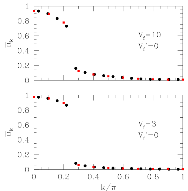
Figure 10: (Color online) Time average of the momentum distribution for $L=20$ (squares) and $L=32$ (circles) for $V_{f}=3$ (bottom panel) and $V_{f}=10$ (upper panel).

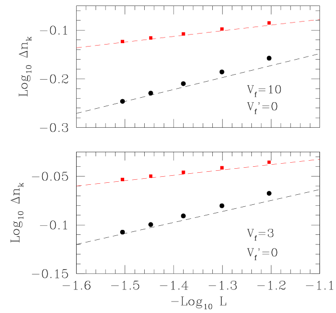
Figure 11: (Color online) Size scaling of the jump at $q=k_{F}$ in the time average of the momentum distribution. Results for $V_{f}=3$ (bottom panel) and $V_{f}=10$ (upper panel) are reported (full circles). The results for the ground state (squares) are also reported for comparison. The slope of the lines corresponds to the critical exponents predicted by bosonization.

We note that the available sizes are sufficient to obtain a very accurate determination of the exponent for the ground state, where the exact values can be computed by Bethe Ansatz. On the contrary, a similar fit for the time averaged results appears to be more problematic, as shown in Fig. 11. Indeed, a pure power-law fit of the data appears to be less accurate and the resulting exponent $\alpha$ increases when the fit is limited to the largest sizes. Nevertheless, Fig. 11 shows that the bosonization approach provides a value for $\alpha$ roughly consistent with the numerical analysis, in agreement with very recent density-matrix renormalization group calculations. karrasch2012 However, we remark that a complete smoothing of the curve at larger sizes cannot be excluded by the Lanczos data.

Finally, we consider the effects of a finite $V_{f}^{\prime}$ in the final Hamiltonian. When sufficiently large, this term is expected to break the integrability conditions. In this case, thermalization should be expected on general grounds and we are in the position to verify whether some evidence for that is already visible on the lattice sizes studied by Lanczos diagonalization. In Figs. 12 and 13, we report the results for ${\overline{N}}_{q}$ and ${\overline{n}}_{k}$, respectively. Three different values of the final interaction strengths are reported. In all cases, ${\overline{N}}_{q}={\rm const}$ for $q\to 0$, while a sizable peak is still present at $q=2k_{F}$. Therefore, the qualitative picture of the previous integrable model holds also in this case.

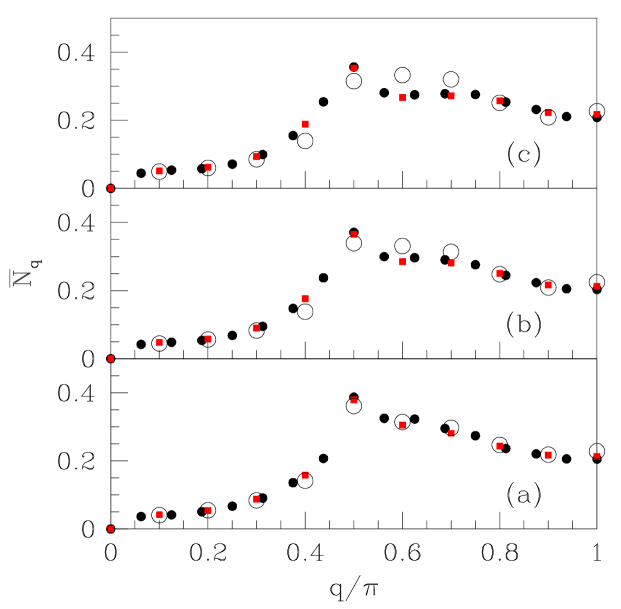
Figure 12: (Color online) Time average of density-density correlation $N_{q}(t)$ for a quench from $V_{i}=0$ to $V_{f}=10$ and $V^{\prime}_{f}=3$ (a), $V_{f}=15$ and $V^{\prime}_{f}=4.5$ (b), and $V_{f}=20$ and $V^{\prime}_{f}=6$ (c). Data for $L=20$ (squares) and $L=32$ (circles) are shown. Thermal values corresponding to an effective temperature that gives the correct internal energy are also shown (empty circles).

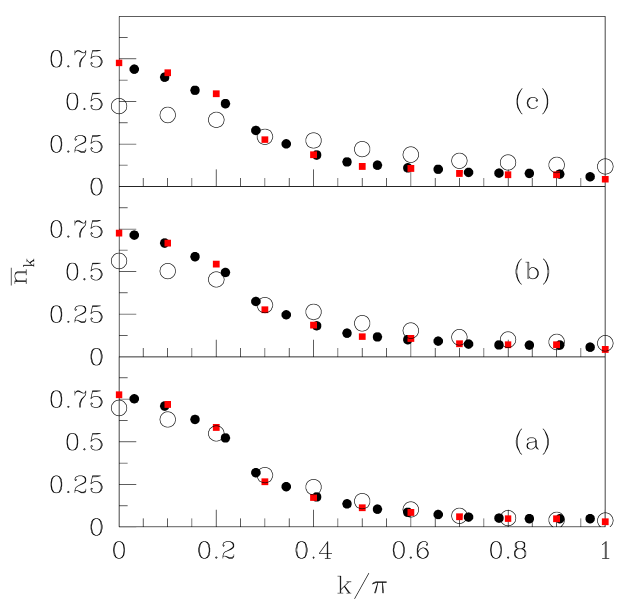
Figure 13: (Color online) Same as in Fig. 12 for the momentum distribution $n_{k}(t)$.

We also notice that, for small quenches (e.g., $V_{f}=10$ and $V^{\prime}_{f}=3$), both the density-density correlations and the momentum distribution may be nicely fitted by assuming a single effective temperature within the canonical ensemble, see Figs. 12 and 13. Indeed, by choosing the temperature that reproduces the value of the internal energy, we are able to obtain a quite satisfactory representation for all momenta, at variance with the integrable case, $V^{\prime}_{f}=0$. Of course, in order to show that a real thermalization takes place, one must show that all correlation functions are described by a single effective temperature. In this respect, the best way is to consider the properties of the (reduced) density matrix, as suggested by Poilblanc in a recent work. poilblanc2011 This task is beyond the scope of the present paper, which is centered around the comparison between the TL model and a microscopic model on the lattice.

For larger quenches, an accurate description of these correlation functions in terms of a single effective temperature is less accurate (see Figs. 12 and 13) and quite substantial deviations from the thermal values are observed for large momenta in the density-density correlations and for small momenta in the momentum distribution.

7 Conclusions

In conclusion, we reported a direct comparison of the non-equilibrium dynamics between the bosonization approach and exact diagonalizations for an interacting model of spinless fermions. On the one hand, we showed that the bosonization technique does not capture few important aspects of the long-time behavior. In particular, a thermal-like behavior of the density-density correlations at small momenta is observed in the numerical calculations (i.e., ${\overline{N}}_{q}\simeq{\rm const}$). On the other hand, our numerical calculations point towards the occurrence of a singularity at the Fermi wavevector in the momentum distribution, as predicted by bosonization. Our conclusions do not crucially depend upon the presence of a next-nearest-neighbor interaction $V^{\prime}$ that breaks integrability, and show that the critical behavior predicted by the bosonization technique should be considered with care and may strongly depend upon the linearization of the fermionic band. The numerical analysis for non-integrable models is consistent with thermalization in the thermodynamic limit, however, significant size effects hamper the possibility to quantitatively investigate the thermalization dynamics.

We thank M. Fabrizio, G. Santoro and A. Silva for stimulating discussions. E.C. also thanks SNSF (Division II, MaNEP).

Appendix A The Jastrow wave function

In this Appendix, we show that the ground-state wave function (15) of the Tomonaga-Luttinger Hamiltonian may be rewritten as a Jastrow term acting on the non-interacting ground state $|0\rangle_{ab}$, i.e., in the form: tayo2008

$$|0\rangle_{\alpha\beta}\propto\exp{\left[\frac{1}{L}\sum_{q>0}w_{q}n_{q}n_{-q}\right]}|0\rangle_{ab},$$ (35)

where the density operators are defined by $n_{\pm q}=\rho(\pm q)=\rho_{L}(\pm q)+\rho_{R}(\pm q)$. Most importantly, we also show that the exact time evolved state (17) can be also written as a (time-dependent) Jastrow term acting on $|0\rangle_{ab}$.

Let us start with the ground state. In order to find out the expression of the pseudo-potential $w_{q}$, on the one hand, we write $|0\rangle_{\alpha\beta}$ by using Eqs. (11) and (12):

$$|0\rangle_{\alpha\beta}\propto\exp{\left[-\frac{v}{u}\sum_{q>0}(ua_{q}^{\dagger}+vb_{q})(va_{q}+ub_{q}^{\dagger})\right]}|0\rangle_{ab}.$$ (36)

On the other hand, we use the fact that:

$$n_{q}n_{-q}=\frac{qL}{2\pi}(a_{q}a_{q}^{\dagger}+b_{q}^{\dagger}b_{q}+a_{q}b_{q}+b_{q}^{\dagger}a_{q}^{\dagger}).$$ (37)

Since, in a Tomonaga-Luttinger liquid, different modes labeled by $q>0$ are not coupled, we can focus our attention on a generic mode, dropping the label $q$. We want to see whether, for a suitable choice of the amplitude $w_{q}$, the expression in Eq. (35) coincides with that of Eq. (36). A solution exists if it is possible to define an amplitude $f$ such that the following equality holds:

$$e^{f(a^{\dagger}a+b^{\dagger}b+ab+b^{\dagger}a^{\dagger})}|0\rangle_{ab}\propto e^{x(aa^{\dagger}+b^{\dagger}b+\nu ab+\frac{1}{\nu}b^{\dagger}a^{\dagger})}|0\rangle_{ab}$$ (38)

for all choices of $x$ and $\nu$. In the case of interest, due to Eq. (36) we have $x=-v^{2}$, $\nu=v/u$, while Eqs. (35), and (37) give $f=w_{q}q/(2\pi)$. Via some lengthy algebra it is possible to show that Eq. (38) is satisfied by the choice:

$$w_{q}=-\frac{2\pi v}{q(u-v)},$$ (39)

in agreement with the results of Ref. tayo2008 . The explicit form of the Jastrow pseudo-potential shows a long-range (density-density) repulsion, with a logarithmic decay in real space:

$$|0\rangle_{\alpha\beta}\propto\exp{\left[-\frac{2\pi}{L}\sum_{q>0}\frac{v}{q(u-v)}n_{q}n_{-q}\right]}|0\rangle_{ab}.$$ (40)

Let us now consider the time evolution and show that the time evolved wave function can be written as a time-dependent Jastrow term applied to the non-interacting state. This can be easily proved by considering Eq. (38) with $x=v^{2}(e^{-2i\epsilon_{q}t}-1)$, $\nu=v/u$, and $f=w_{q}(t)q/(2\pi)$. The final result reads as:

$$e^{-i{\cal H}t}|0\rangle_{ab}\propto\exp{\left[\frac{1}{L}\sum_{q>0}w_{q}(t)n_{q}n_{-q}\right]}|0\rangle_{ab},$$ (41)

with

$$w_{q}(t)=\frac{2\pi v}{q(u-v)}\left[\frac{u(e^{-2i\epsilon_{q}t}-1)}{u+ve^{-2i\epsilon_{q}t}}\right].$$ (42)

Therefore, we obtain the important result that the exact time evolution of $|0\rangle_{ab}$ under the action of ${\cal H}$ can be written as a Jastrow wave function, with a complex time-dependent pseudo-potential $w_{q}(t)$.

References

- (1) M. Greiner, O. Mandel, T.W. Hansch, and I. Bloch, Nature 419, 51 (2002).
- (2) T. Kinoshita, T. Wenger, and D.S. Weiss, Nature 440, 900 (2006).
- (3) S. Hofferberth, I. Lesanovsky, B. Fischer, T. Schumm, and J. Schmiedmayer, Nature 449, 324 (2007).
- (4) S. Trotzky, Y.-A. Chen, A. Flesch, I.P. McCulloch, U. Schollwock, J. Eisert, and I. Bloch, Nature Physics 8, 325 (2012).
- (5) A. Polkovnikov, K. Sengupta, A. Silva, M. Vengalattore, Rev. Mod. Phys. 83, 863 (2011).
- (6) P. Barmettler, M. Punk, V. Gritsev, E. Demler, and E. Altman, Phys. Rev. Lett. 102, 130603 (2009).
- (7) M. Rigol, V. Dunjko, and M. Olshanii, Nature 452, 854 (2008).
- (8) For a recent review, see for example, M. A. Cazalilla, R. Citro, T. Giamarchi, E. Orignac, and M. Rigol, Rev. Mod. Phys. 83, 1405 (2011) and reference therein.
- (9) M.A. Cazalilla, Phys. Rev. Lett. 97, 156403 (2006).
- (10) C. Kollath, A.M. Lauchli, and E. Altman, Phys. Rev. Lett. 98, 180601 (2007).
- (11) S.R. Manmana, S. Wessel, R.M. Noack, and A. Muramatsu, Phys. Rev. Lett. 98, 210405 (2007).
- (12) P. Calabrese, F.H.L. Essler, and M. Fagotti, Phys. Rev. Lett. 106, 227203 (2011).
- (13) The standard way to define quantum integrability is by having scattering without diffraction, see B. Sutherland, Beautiful Models (World Scientific, Singapore, 2004). For a more recent discussion, see for example, E.A. Yuzbashyan, B.S. Shastry, arXiv:1111.3375 and references therein.
- (14) M. Rigol, V. Dunjko, V. Yurovsky, and M. Olshanii, Phys. Rev. Lett. 98, 050405 (2007).
- (15) J.M. Luttinger, J. of Math. Phys. 4, 1154 (1963).
- (16) E.H. Lieb and D.C. Mattis, J. of Math. Phys. 6, 304 (1965).
- (17) A. Luther and I. Peschel, Phys. Rev. B 9, 2911 (1974).
- (18) F.D.M. Haldane, Phys. Rev. Lett. 45, 1358 (1980).
- (19) F.D.M. Haldane, J. Phys. C 14, 2585 (1981).
- (20) T. Giamarchi, Quantum Physics in One Dimension, Oxford University Press (2004).
- (21) C. Karrasch, J. Rentrop, D. Schuricht, and V. Meden, Phys. Rev. Lett. 109, 126406 (2012).
- (22) A. Mitra and T. Giamarchi, Phys. Rev. Lett. 107, 150602 (2011).
- (23) R. Jastrow, Phys. Rev. 98, 1479 (1955).
- (24) M. Capello, F. Becca, M. Fabrizio, S. Sorella, and E. Tosatti, Phys. Rev. Lett. 94, 026406 (2005).
- (25) M. Capello, F. Becca, M. Fabrizio, and S. Sorella, Phys. Rev. Lett. 99, 056402 (2007).
- (26) G. Carleo, F. Becca, M. Schiró, and M. Fabrizio, Scientific Reports 2, 243 (2012).
- (27) We stress the fact that the model with is integrable and, therefore, a complete thermalization is not possible. Nevertheless, some aspects of a thermal-like behavior can be seen in some correlation functions.
- (28) I. Affleck, D. Gepner, H.J. Schulz, and T. Ziman, J. Phys. A 22, 511 (1989).
- (29) S. Sorella, A. Parola, M. Parrinello, and E. Tosatti, EPL 12, 721 (1990).
- (30) D. Poilblanc, Phys. Rev. B 84, 045120 (2011).
- (31) B. Tayo and S. Sorella, Phys. Rev. B 78, 115117 (2008).