A Heterogeneous Accelerated Matrix Multiplication: OpenCL + APU + GPU+ Fast Matrix Multiply

Abstract

As users and developers, we are witnessing the opening of a new computing scenario: the introduction of hybrid processors into a single die, such as an accelerated processing unit (APU) processor, and the plug-and-play of additional graphics processing units (GPUs) onto a single motherboard. These APU processors provide multiple symmetric cores with their memory hierarchies and an integrated GPU. Moreover, these processors are designed to work with external GPUs that can push the peak performance towards the TeraFLOPS boundary.

We present a case study for the development of dense Matrix Multiplication (MM) codes for matrix sizes up to 19K$\times$19K, thus using all of the above computational engines, and an achievable peak performance of 200 GFLOPS for, literally, a made-at-home built. We present the results of our experience, the quirks, the pitfalls, the achieved performance, and the achievable peak performance.

P. D’Alberto. OpenCL+APU+GPU+FastMM

Author’s addresses: P. D’Alberto paolo@FastMMW.com

1 Introduction

As users and consumers, we are accustomed to having multiple cores in a single processor and we are enjoying the many advantages. Nowadays, processors with two or more cores are common in notebooks, tablets and smart phones, delivering additional performance. Desktops may have 4-8 core processors, servers usually have multi-core processors as well. Also, as occasional gamers, either through casual games played in a browser or multiplayer games played on a console or PC, graphics processing units provide those realisitic effects we are used to and take for granted.

As developers and algorithm designers, we are experiencing a kind of Renaissance because we are stimulated to design algorithms to exploit these new computational engines for both new and old applications. A Renaissance indeed, because super computing is not anymore at the fingertips of only a small elite but it is practically for everyone. Think, anyone capable to use a screw driver could build a desktop capable to deliver one and more TeraFLOPS peak performance with a few GPUs in it [Vetter et al. (2011)]; paraphrasing Cray’s saying: we have a few oxes pulled by hundred of chickens. The last attempt to do such a popularization of supercomputing was by the Cell processor and the PS3 game console (which became impossible for future systems as SONY removed support for the LINUX operating system) achieving the same performance by the same flop per dollar ratio that we shall present in this work.

In this work, we turn our attention to heterogeneous systems and in particular to single board systems with hybrid processors, that is with symmetric cores and a GPU, and additional external GPUs; we call these computational engines; each computation engine will have very different performances and will fit very different computational needs. Here, we can easily add or substitute computational engines in the system: for example, we can change a GPU by a snap (or two) and we want software to change the work load accordingly even at run time. Note, in this type of systems, the GPU is one component. In particular, the external GPUs can be omitted altogether and still have GPU capabilities. Moreover, as the technology improves, we may easily pluck out the APU processor for a new version, with larger GPU within or more cores. This upgrade of the system is more in line with small budgets planning, where only a part of the machine is upgraded, not decommissioned, and the rest is left unchanged. The ability to write code that, in principle, adapts to the different configurations with little or no modifications will make these systems even more appealing: simplifying costly software maintenance.

We neither measure nor present in-GPU timing (AMD OpenCL package provides examples of how to measure the internal computation time only but we wanted to measure the so called wall-clock as well). We take the point of view that GPUs and APUs are accelerating devices, thus we should present the overall acceleration in combination with classic computation (non-accelerated or CPU-only) so to appreciate the organic performance. Of course, the performance will be less jaw dropping, it will be sober and reasonable, nonetheless impressive. After all, we are interested in those types of computations where the transfer of data and its execution time (of the transfer) are integral parts of the computation. To be fair, we measure performance for problem sizes that are very large and they will not fit in any computation-engine internal memory.

We will take an agnostic view of the GPUs and the code for them. In fact, we are going to use OpenCL to abstract the system resources and we will use the OpenCL interface to guide the computations. Also, we are going to take the MM Kernels provided within the OpenCL samples as they are. What we are after is the ability to determine the capacity storage of the GPUs or internal memory. Thus, we are interested in the workload capability of the GPUs and we will reuse the code available. We shall go into the details in in Section 3.1.

We are going to use a different attitude about the code for the CPUs. We will reuse the code provided by ATLAS and GotoBLAS. That is, we are going to use the best known codes for multi-core systems. We will deploy with our codes the SGEMM’S from ATLAS because of a conflict with thread allocation using GotoBLAS. However, we will provide the performance for both so that to appreciate the hardware-accelerators effects.

We choose to present performance for the Matrix Multiplication kernel because: First, it is a well known kernel; second, there are close to optimal codes for both GPUs and CPUs; third, we are interested in the interrelation among CPUs and GPUs, which is a relatively new problem; and fourth, we are interested to investigate how close we can get to the peak performance.

The challenges to solve are not new and they are not trivial either. We shall show a natural and simple approach to take advantage of the diversity of the computational engines and we shall show that all engines are useful in different ways: First, CPUs will provide the best solution for relatively small problems; second, all GPUs should be used for the solution of intermediate and large problems; finally, CPUs will support coordination and data-layout transformations necessary for the handling of very large problems.

We organize our work as it follows. In Section 2, we shall try our best in providing a survey about the related work. In Section 3, we shall introduce our contribution and system in a top-down fashion: in Section 3.1, we shall present the recursive algorithm that will break down the computation in smaller ones to be solved by the computational engines; in Section 3.2, we shall provide the details how we combine the power of the different engines; in Section 3.3, we shall describe how we use OpenCL to abstract the computational engines, and in Section 3.4 we shall provide details about the hardware we deployed. In Section 4, we shall present our experimental results: as peak performance, in Section 4.2, and as achievable performance, in Section 4.3. We conclude with our acknowledgments.

A note: In this work, we will not discuss nor present any numerical analysis such as maximum error, maximum relative error.

2 Related Work

We can divide this section into several parts: For example, about the Matrix Multiplication and its applications, about implementations of MM for multi-core multi-processors, about implementation for GPUs, Software/Hardware hybrid implementations where desktop solutions are combined with low power field programmable gates FPGAs solutions. In fact, MM is so ubiquitous in science that it is used very often as kernel, as a basic operation, and also as a benchmark for new systems, for new architectures. This exposure of MM in different fields and the simplicity how MM can be presented make MM like a common language and often it is taken for granted; at the same time, it is also like a secret hand-shake for researcher communities, among who a very few researchers have mastered it really.

Matrix Multiplication is considered such an old-school problem but it still attracts a large volume of research. We are all familiar with the algorithm of complexity $O(N^{3})$, which is the standard implementation in the NETLIB BLAS. In turn, BLAS 3, the set of matrix-matrix operation can be reduced to matrix multiplication [Kagstrom et al. (1998), Blackford et al. (2002)]. Optimized BLAS are extremely useful and ubiquitous in scientific and statistical software packages, often we may used them without know it. In this work, we work with ATLAS [Whaley and Dongarra (1998)] and with GotoBLAS [Goto and van de Geijn (2008)]. We are interested in the so called Fast MM algorithms: Vassilevska-Williams [Williams (2011)] Coppersmith-Winograd’s [Coppersmith and Winograd (1987)], Pan’s [Pan (1978)], Strassen’s [Strassen (1969)], and our recent implementations for SMP machines [D’Alberto et al. (2011)]. Fast MM are practical and stable [Demmel et al. (2006), Demmel and Higham (1992)]. The connection between MM and other applications can be surprising: for example in a semi-ring (where the $+$ operation may not have inverse) the All-Pair shortest-path and the classic MM are computationally equivalent and they have the same solution [D’Alberto and Nicolau (2007), Warshall (1962), Floyd (1962)]. The connection was not lost in the implementation for GPUs [Buluç et al. (2008)].

MM has been used a benchmark or as motivational example for compiler optimizations such as tiling, parallelism by threads manually or automatically by OpenMP [Chandra et al. (2000)] or Cilk [Frigo et al. (2009)]. Other optimizations in combination with the above is matrix layout optimizations [Chatterjee et al. (2002)], which we could take advantage in this work as well.

The parallelism of MM is a central subject of this work. For Fast MM, the authors have a recent contribution to exploit the full speed up in symmetric multi-core processors [D’Alberto et al. (2011)]. In that work, symmetry of the architecture and of the algorithm is fundamental for achieving the best performance. Here, in contrast, asymmetric computational engines are part of the architecture. The software must be aware and adapt.

Currently, GPUs are having more and more traction in the scientific computing as flexible means to compute complex algorithms and, especially, as computational engine with jaw-dropping performance reaching easily 500GFLOPS. The literature is rich of fast GEMM implementations of MM [Tan et al. (2011), Li et al. (2009), Volkov and Demmel (2008)], Fast MM [Li et al. (2011)], and fast and accurate [Badin et al. (2011)].

What actually attracted us to this subject —i.e., MM for heterogeneous computing— has been the arrival on a new architecture such as the APU [Brookwood (2010)] and the OpenCL [Gaster et al. (2011)] as a programming environment/API. Using OpenCL, AMD OpenCL examples, and a little practice, we could run code for both the CPUs and the GPUs, without knowing the inner workings of neither. Considering that the high performance codes for the CPUs took a decade to reach the level they are now, the ability to write code for even more complex system is quite something.

From the exchange of emails with other researchers who have asked for our Fast MM codes, we have noticed that such an ease to code can tempt developer to use a single code for all devices. This is a cheap solution, the code is easy, there is no maintenance but the performance and efficiency will be poor defying the purpose of these beautiful machines.

3 Top-Down Matrix Multiplication

We opt to present our system in a top-down fashion. We start by presenting the classic recursive algorithm for the computation of Matrix Multiplication (Section 3.1). The recursive algorithm, when reaching an appropriate problem size, will yield control to a leaf computation (Section 3.2). The leaf computation can be a CPU only computation, GPUs only computation, and GPUs and CPUs. The leaf computation is based on an abstraction of the computational engines as we present in Section 3.3. We describe the hardware of our system, the possible configurations and we show a picture of the build in Section 3.4.

3.1 Recursive Description

Our goal is to compute matrix multiplication for any problem size with the help of different computational engines. In this work, we use a recursive algorithm that is designed to divide the problem in similar sub-problems using a recursive formulation. We actually have two recursive algorithm explicitly computing the single MM and the multiply-add matrix computation, see Table 3.1.

Note that the algorithm stems from the observation that any matrix ${\bf D}\in\mathbb{R}^{m\times n}$ can be always divided into four quadrants:

$${\bf D}=\begin{bmatrix}{\bf D}_{0}&{\bf D}_{1}\\ {\bf D}_{2}&{\bf D}_{3}\\ \end{bmatrix}.$$ (1)

Here, we divide the matrix so that ${\bf D}_{0}\in\mathbb{R}^{\lceil\frac{m}{2}\rceil\times\lceil\frac{n}{2}\rceil}$ and ${\bf D}_{3}\in\mathbb{R}^{\lfloor\frac{m}{2}\rfloor\times\lfloor\frac{n}{2}\rfloor}$.

Matrix Multiplication ${\bf C}={\bf A}{\bf B}$ descriptions. ${\bf C}={\bf A}{\bf B}$ ${\bf C}{+=}{\bf A}{\bf B}$ if small then Leaf(${\bf C},{\bf A},{\bf B}$) if small then LeafAdd(${\bf C},{\bf A},{\bf B}$) else else         ${\bf C}_{0}={\bf A}_{0}{\bf B}_{0}$         ${\bf C}_{0}{+=}{\bf A}_{0}{\bf B}_{0}$         ${\bf C}_{1}={\bf A}_{0}{\bf B}_{1}$         ${\bf C}_{1}{+=}{\bf A}_{0}{\bf B}_{1}$         ${\bf C}_{2}={\bf A}_{2}{\bf B}_{0}$         ${\bf C}_{2}{+=}{\bf A}_{2}{\bf B}_{0}$         ${\bf C}_{3}={\bf A}_{2}{\bf B}_{1}$         ${\bf C}_{3}{+=}{\bf A}_{2}{\bf B}_{1}$         ${\bf C}_{0}{+=}{\bf A}_{1}{\bf B}_{2}$         ${\bf C}_{0}{+=}{\bf A}_{1}{\bf B}_{2}$         ${\bf C}_{1}{+=}{\bf A}_{1}{\bf B}_{3}$         ${\bf C}_{1}{+=}{\bf A}_{1}{\bf B}_{3}$         ${\bf C}_{2}{+=}{\bf A}_{3}{\bf B}_{2}$         ${\bf C}_{2}{+=}{\bf A}_{3}{\bf B}_{2}$         ${\bf C}_{3}{+=}{\bf A}_{3}{\bf B}_{3}$         ${\bf C}_{3}{+=}{\bf A}_{3}{\bf B}_{3}$

In this work, we shall present results for square matrices, however the recursive algorithm is oblivious of the shape of the matrices. Furthermore, the division of matrices into balanced sub-matrices is the foundation of fast algorithm and thus we could always use a fast algorithm presented in previous work without any modification of the leaf computation. But this is beyond the scope of this investigation.

The goal of a balanced recursive algorithm is simplicity and recursive tiling. In contrast, tiling of the classic MM divides the problem into smaller sub-problems and mostly of fixed size. Classic tiling could provide better performance for a given architecture but less flexibility. At this level of the computation, we rather have the latter and compromise a little with the former.

In Table 3.1, we omitted the details of when the problem size is small. In naive terms, we would like to yield to the leaf computation when either the CPUs or the GPUs can handle the problem at hand directly. In this work, the recursion stops when the operands matrix size is smaller than $6016\times 6016$, this is also called recursion point. We shall dwell into the details in the experimental section, when the architecture will be clear. Intuitively, the recursion is chosen so that both the internal GPU and the external GPU can provide almost peak performance.

3.2 Leaf Computation

We turn our attention to the leaf computation that performs the MM ${\bf C}={\bf A}{\bf B}$. The leaf computation is simple to describe:

Leaf(C,A,B) Leaf$({\bf C},{\bf A},{\bf B})$ if size $\geq K_{1}$         rGPUs(C,A,B) if size $\geq K_{0}$ and size $<K_{1}$         GPU(C,A,B) otherwise         SGEMM(C,A,B)

Let us recall that we are working with a system composed of an APU and an external GPU. That is, we have two GPUs, one is internal to the APU and the other is external.

If the problem size is larger than a critical point, we will use either a single or multiple GPUs to solve the problem; otherwise, we call SGEMM (from any high performance BLAS 3 library).

Let us address the small problem first. Experimentally and for this architecture, if the matrices are smaller than $400\times 400$ (i.e., $K_{0}=400$) we are better off using SGEMM: we took in consideration both ATLAS and GotoBLAS. We eventually decided to use ATLAS because GotoBLAS affects the thread allocation in OpenCL adversely by serializing the GPU computations. However, we shall show that GotoBLAS SGEMM standalone is faster than the ATLAS counterpart. In the experimental section, we shall provide more details.

For problem sizes larger than $K_{0}=400$ and smaller than $K_{1}\sim 3000$ we will use a single GPU, the external one. In the following, Section 3.3, we will provide the details the GPU MM kernel. The choice of the breaking point $3000$ is small with respect to the capacity of the external GPU, which can solve MM with matrices up to $4300\times 4300$. The size $3000$ is the break-even point when both GPUs should work collaboratively and also the problem size that the internal GPU can solve directly. In our system, the GPU crossfire is activated, thus boosting the throughput and thus the parallelism between the GPUs.

Now, let us address the computation using GPUs, which is at the center of our work. Once again the idea is simple. Consider the problem ${\bf C}={\bf A}{\bf B}$, we can split the matrices as follows.

$$\begin{bmatrix}{\bf C}_{0}&{\bf C}_{1}\\ {\bf C}_{2}&{\bf C}_{3}\\ \end{bmatrix}=\begin{bmatrix}{\bf A}_{0}&{\bf A}_{1}\\ {\bf A}_{2}&{\bf A}_{3}\\ \end{bmatrix}*\begin{bmatrix}{\bf B}_{0}&{\bf B}_{1}\\ {\bf B}_{2}&{\bf B}_{3}\\ \end{bmatrix}.$$ (2)

and thus we can allocate to one GPU the following computation:

$${\bf C}_{0}={\bf A}_{0}*{\bf B}_{0};\hskip 5.69046pt{\bf C}_{0}+={\bf A}_{1}*{\bf B}_{2};\hskip 5.69046pt{\bf C}_{2}={\bf A}_{2}*{\bf B}_{0};\hskip 5.69046pt{\bf C}_{2}+={\bf A}_{3}*{\bf B}_{2}$$ (3)

and to the other the smaller computation:

$${\bf C}_{1}={\bf A}_{0}*{\bf B}_{1};\hskip 5.69046pt{\bf C}_{1}+={\bf A}_{1}*{\bf B}_{3};\hskip 5.69046pt{\bf C}_{3}={\bf A}_{2}*{\bf B}_{1};\hskip 5.69046pt{\bf C}_{3}+={\bf A}_{3}*{\bf B}_{3}.$$ (4)

The matrices do not need to be square. Nonetheless, the computation is balanced, in the sense that ${\bf C}_{0}={\bf A}_{0}*{\bf B}_{0}$ computes just $N^{2}$ operations more than ${\bf C}_{3}+={\bf A}_{3}*{\bf B}_{3}$, where $N\times N$ is the matrix size of ${\bf C}_{0}$. This difference is in the matrix-vector computations needed to compute the borders of ${\bf C}_{0}$, which account for $2N-1$ extra elements.

In general, this does not need to be: one GPU could work on a problem much larger than the other. We tested such an unbalance division but, for our system, it did not provide any performance advantage and thus we do not discuss it any further.

A simple optimization, for which we will present results in a future work, is the change of layout of the operands so that the sub matrices —i.e., ${\bf C}_{0},{\bf C}_{1},{\bf C}_{2}$, and ${\bf C}_{3}$— are continuous in memory. The advantage is two fold: the change of layout is used by both GPU computations, thus we can save communications, and this will speed up the communication between memory and the GPU internal memory.

3.3 OpenCL Configuration

We abstract our system by using platforms, queues, and devices. A platform is composed by devices: CPUs and GPUs. A platform can have multiple devices: In this work we work with an internal CPU device, an internal GPU device (we shall use the term $GPU_{1}$), and an external GPU device ($GPU_{0}$). In particular, we use OpenCL to abstract only GPU devices. Any device is identified by an unique integer and the basic information about the device can be queried using this unique identifier. We associate to every GPU device a Matrix Multiplication queue structure.

A MM queue will collect basic information about the device such as the size of the internal memory, if it has any. The MM queue will have the function of an OpenCL queue: Memory context, memory buffers, programs or kernels, and command queue.

We built a system that has three devices (CPU, $GPU_{1}$ and $GPU_{0}$). We consider the two GPUs like a priority queue: where we serve first and with larger problem the $GPU_{0}$ and then $GPU_{1}$. We query the information about the devices and in particular we determine the internal data buffer in such a way we estimate the problem size that a device will be able to solve. The internal $GPU_{1}$ can store three matrices of size $3008\times 3008$, thus a square problem size of $N=3008$. The external $GPU_{0}$ can solve a larger problem: that is, $N=4305$. Such a capacity of the GPUs is fundamental for the division strategy and it is determined and exploited at run time.

To initialize a MM queue, we create a context and a command queue first. A context is an abstract object that manages the interaction between the host (program) and the devices such as memory objects in a device and kernel programs created for a device. A command queue is the main mechanism to communicate, to start a computation, and to control a device. Then, we create the buffers and the codes. We create three buffers, which are contiguous memory that the device uses as transient memory to read the matrix operands and to write the matrix result. We compile OpenCL programs for MM that are available through the AMD OpenCL distribution. We modified the programs a little to adapt to a few new requirements, but the modifications are minor.

Once the MM queue is initialized, we are ready to execute commands; for example, the matrix computation ${\bf C}+={\bf A}{\bf B}$ is performed by three basic MM queue routines in order:

1. Move the operands ${\bf A}$ and ${\bf B}$ into the input buffers and wait for the communication completion.

2. Execute the basic MM kernel, ${\bf C}={\bf A}{\bf B}$, which is like an external function call.

3. Move the output into a local memory space and add ${\bf C}$.

We believe that the communication operations (moving the input matrices and output matrix) are intuitive to grasp without too many details, especially if the matrix operands are contiguous in memory. We believe that the kernel execution is less intuitive and it deserves more details.

First, let us recall that we are working with GPU engines and thus the computation should be designed for this graphic unit. As intuitive description, we can divide the computation into three parts: the splitting of the computation into threads, the instantiation of the parameters, and then the actual queuing of the kernel for execution. Of course, we will wait for the completion of the execution before to return. This is identical, at least in principle, to a function call.

The main difference with a function call is the initial division of the original computation into threads. This division is only nominal in the sense that is not apparent at code level but the GPUs internal mechanism will carry it on: Consider the result matrix ${\bf C}$, if we divide the matrix into four quadrants as previously, we can divide the computation into four independent computations or threads, each thread will compute a blocked row-by-column matrix multiplications such as

$${\bf C}_{0}={\bf A}_{0}*{\bf B}_{0}+{\bf A}_{1}*{\bf B}_{2}.$$ (5)

The number of threads, that is, how we divide the matrix ${\bf C}$, depends on the type of GPUs basically. Each computation is often implemented by the classic MM row-by-column operation. In principle, each thread could be computing a single point of ${\bf C}$ like this:

$$c_{i,j}=\sum_{k=1}^{N}a_{i,k}b_{k,j}$$ (6)

In this work, the kernel computes a $32\times 32$ tile of ${\bf C}$. This division process is natural in the field of loop parallelization: we parallelize the outer loop of the classic MM (three for-loops), which is common using OpenMP pragmas. This is not necessarily the best strategy and a blocked version could provide better raw FLOPS performance and also achieving smaller numerical error.

3.4 Hardware

The system built has the following specifications

• 16GB Memory 4Gx4|CORSAIR CMZ8GX3M2A1866C9B2Z

• Motherboard ASUS|F1A75-M PRO R1

• Processor A8-3850

  • 4 CPUs

  • AMD Radeon HD 6550

  • Off-market CPU cooler Hyper 212 plus

• External GPU, Diamond Radeon HD 6570

In Figure 1, we show literally a snapshot of the built system.

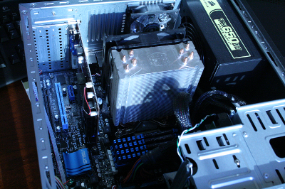
Figure 1: Board snapshot

Through the BIOS of the ASUS motherboard, we can set the default base clock and thus configure the system. We tried a few, in Table 3.4, we show the ones stable so that we could run experiments.

Configurations Base Clock mult. Default 90 100 112 114 115 APU MHz (peak) 2900 2610 2900 3248 3306 3335 Memory MHz 1333 1440 1600 1792 1824 1840

In the following of the paper, we will use the base clock multiplier (i.e., Default, 90, etc) so that to identify the system and present performance. We wrote all the codes independently of the hardware configurations. In practice, we wrote the codes and tune them in the default configuration.

We installed Ubuntu 10.04 Natty, we then installed ATI Catalyst 11.8 and AMD OpenCL pack. The code used in this work is a variation of the already available in the samples distribution. We will provide our codes if requested.

4 Experimental Results

For presentation purposes, we split the section into three subsections. We start with the software only performance; in Section 4.1, we present the performance of GEMM by ATLAS and GotoBLAS. Then, we show the peak performance of the system using only GPUs, in Section 4.2, and what we can achieve when all data transfers are considered, see Section 4.3. Notice that when we talk about peak performance, we do not consider in-GPU timing and we do not consider hypothetical performance by resources counting and throughput only.

We measure performance as GLOPS (giga floating point operation per second). We measure the ratio of the number of operation divided by the wall-clock execution time of the MM. The number of operations is $2N^{3}$ where $N$ is the problem size. We consider square problems for presentation purpose, that is, convenience.

4.1 Peak Performance: CPUs only

The CPU device in the APU provides a four-core system that can be used to run efficient implementations of SGEMM. In this section, we present the performance for SGEMM from the ATLAS and from the GotoBLAS library. Also, we present the performance for the Winograd’s MM as implemented by the same authors in [D’Alberto et al. (2011)] and we shall use the symbol SW. We will show that the same algorithm called in the OpenCL environment will have different performance. The performance presented in this section is measured independently of the OpenCL and its framework.

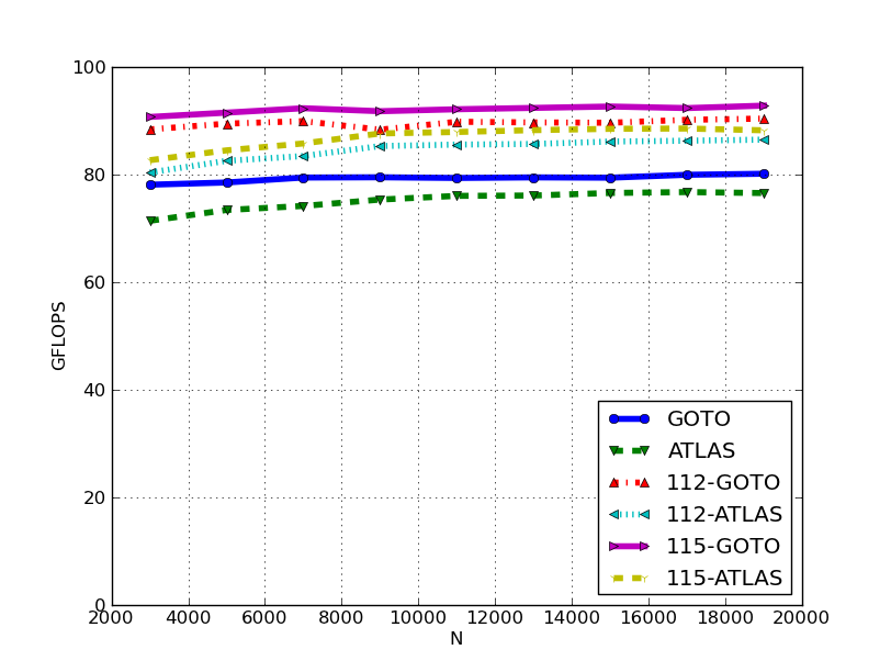
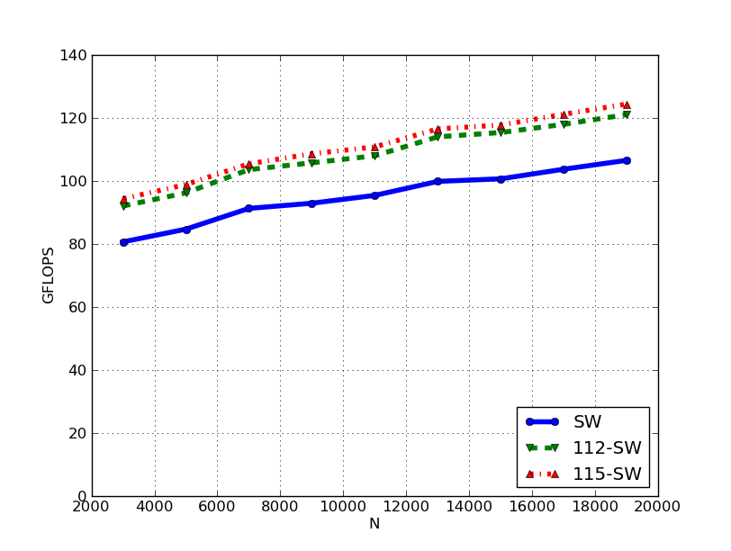
Figure 2: Parallel CPUs: GotoBLAS’s, ATLAS’s SGEMM and Goto-based Winograd’s MM performance

In Figure 2, we can see that the GotoBLAS SGEMM is faster than ATLAS’s SGEMM. For GotoBLAS, we generate code for the Shanghai architecture (i.e., GotoBLAS2) because the APU processor is not recognized in current installation process. ATLAS’s is self tuned and it provides very good performance. ATLAS’s SGEMM is about 5% slower for larger problems and about 10% slower for smaller ones. Our implementation of Winograd implementation is based on Goto’s SGEMM so that to show what could it be the performance by using Algorithm acceleration only.

We can see that SGEMM implemented with the best code for this APU cores run at about 90 GFLOPS. We shall show this performance is about 20 GFLOPS slower that the MM using the internal GPU alone, 30 GFLOPS slower than using the external GPU, and 60 GFLOPS slower than using all. Notice also that we can achieve about 120 GFLOPS using Winograd’s implementation: making it as fast as the internal GPU, which is very competitive.

4.2 Peak Performance: GPUs only

In this section, we address the peak performance that we can achieve using only the GPUs. In particular, we have the matrix operands stored continuously in memory, thus requiring little or no pre-computation. In this way, we can measure the peak performance of the GPUs when the data reside in memory (off the GPUs local storage). In Figure 3, we show the performance we can achieve for every GPU separately with different configurations.

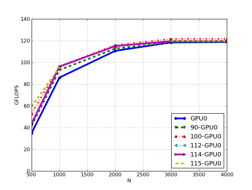
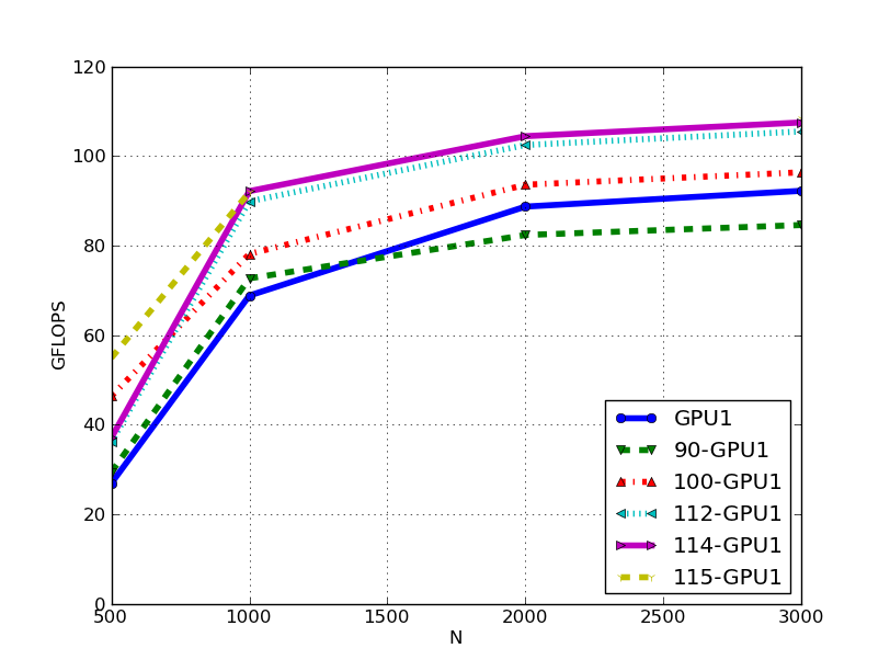
Figure 3: Each GPU performance respectively

We recall the notation used: The $GPU_{0}$ is the external GPU (connected through the PCI) and it can solve directly problems of size up to $4300\times 4300$. The $GPU_{1}$ is the internal GPU and it can compute directly problems of sizes up to $3008\times 3008$.

We notice that $GPU_{0}$ can achieve up to 120GFLOPS peak performance independently of the system configuration. However, for smaller problems a faster memory allows better performance. In contrast, the $GPU_{1}$ improves consistently as the configuration gets faster. There is about 10–30 GFLOPS performance difference between the two GPUs as a function of the configuration.

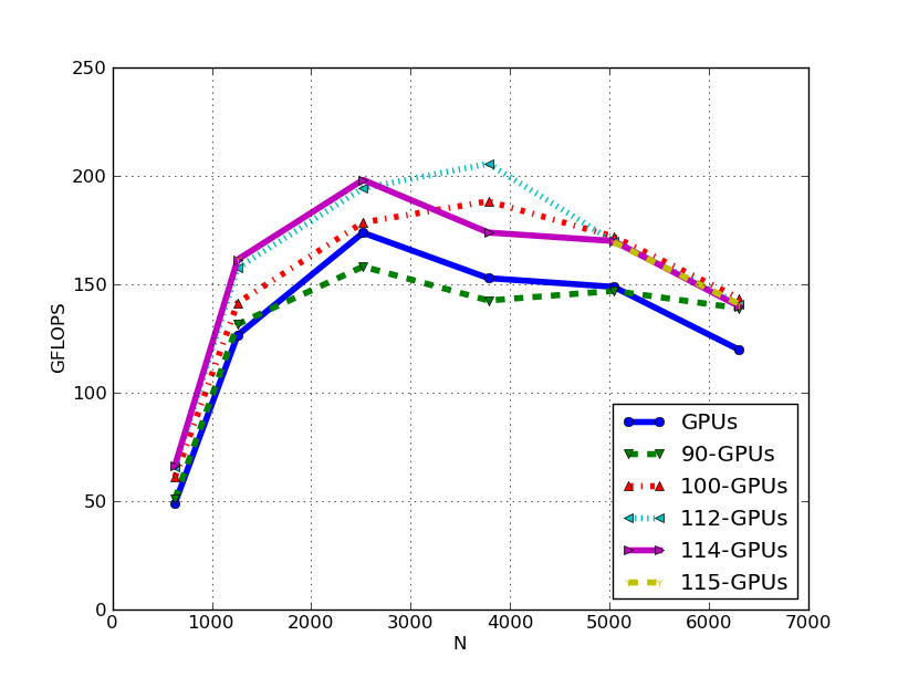
Figure 4: Parallel GPUs performance

In Figure 4, we show the performance when the two GPUs run concurrently on independent MM on matrices stored continuously in memory. This performance graphs needs an introduction and explanation: We took a square problem $N\times N$ and we run it on both GPUs in parallel. The number of operations are $2*(2N^{3})$ and the problem size can be estimated as $2^{\frac{1}{3}}N\times 2^{\frac{1}{3}}N$. In the abscissa of the plot we present $2^{\frac{1}{3}}N$.

Now, we notice right the way that the peak performance is about 200 GFLOPS, but instead of increasing as the problem size increases, it reaches a maximum at about $N=4000$ and then it decreases consistently and for all configurations. It is like the system reaches a bottle neck and the throughput get affected negatively by the communication of data. This makes us believe that, when communications will be integrand part of the computation as in the following section, the practical peak performance could be at about 150 GFLOPS. Notice also that there is no apparent slow down for either one GPU respectively.

In practice, a few configurations are fully stable, and some measures could not be collected reliably especially for the fastest configurations such as 115.

4.3 Accelerators performance

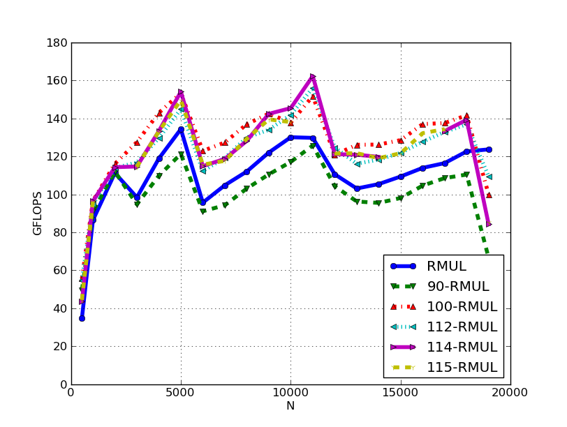
Figure 5: GPUs Accelerated (rmul)

In Figure 5, we present the performance for the recursive algorithm RMUL as we presented in Table 3.1. This figure presents the classic performance curve of a recursive algorithm: a tooth-saw shape. As a function of the original problem size, the leaf computation could be different. Probably, fixed decomposition will have a smaller variance such as between peaks and valleys. The best performance is about 160 GFLOPS, which is about the peak performance we expected (see previous Figure 4). Changing the layout of the operands, when appropriate, could provide smoother performance plots.

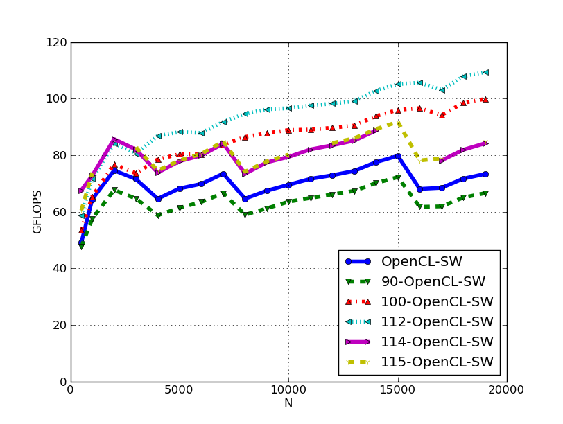
Figure 6: CPU Winograd Accelerated (bmpipe)

Within the OpenCL environment, we measured the performance of the Winograd’s CPU-only MM based on the ATLAS’s SGEMM kernel. In Figure 6, we present the results. We notice quickly that this picture presents a different performance plots (more jagged) than what we presented in Figure 2. At this time, we have no clear explanation but there could be an interaction between the OpenCL environment and the GEMM library.

Instead of using the algorithm in Table 3.1, we could use the fast recursive algorithm based on the Winograd algorithm. The advantages of the fast algorithm will be fewer communication and faster execution time. However, this is beyond the scope of this paper and we shall address such a optimization in a different work.

4.4 Conclusions

In our system, the APU provides a software solution using only CPUS that can achieve 90GFLOPS (GotoBLAS). If we would like to improve performance by just working on a different and fast algorithm, we can achieve 120 GFLOPS. If we take advantage of both GPUs, we can achieve sustainable performance of about 160 GFLOPS (and a peak performance of 200 GFLOPS). This is a first attempt in putting together a OpenCL solution for the implementation of MM using hybrid parallel systems. The heterogeneous system presents interesting challenges and, thanks to the OpenCL API, ultimately a flexible and powerful environment.

The authors are in deep dept to the following people who made this project possible and, most importantly, fun. We thank Matteo Frigo who made the authors aware about the APU architecture. We thank Chris Drome for his encouragement. A heartfelt thank goes to Fred Shubert and the AMD Accelerated Parallel Processing (APP) group who provide an APU sample and support. We thank also Todd Green for reaching out from Morgan Kaufmann about OpenCL. Lastly, we thank Matthew Badin, Alexandru Nicolau, Michael Dillencourt for the conversations about GPUs.

In the following, there are four comments about this work (and reasons for its rejections EuroPar 2012). We see no need for any rebuttal.

======= Review 1 =======

> *** Comments: Comments to author

The method presented in this paper is good. I agree it is suitable for
 that kind of heterogeneous computing environment.

You divide the matrices into four sub-matrices. How better is this in
 case of GPU? This is one of the points we are interested in.

I’m not sure the system works correctly or not with
 over/under-clocking. That can be used to find bottle-neck, however
 not recommended to performance evaluation.

If you are using the advantage of CrossFire, you should mension more
 detail for readers.

Also it is not clear what the CPU threads are doing in two GPU RMUL
 case? Only control and copy/pack/unpack operations?

I could not understand the explanation about the horizontal axis of
 Fig. 3. It seems to exceed the smaller size limit for internal GPU.

The weakness is that, you are using a low-end device for external
 GPU. Usually, we assume external GPU is much faster than internal.

BTW, this is the first time I could not see summary nor conclusion
 section in the paper. Maybe due to lack of pages. We have to estimate
 your main contribution from other parts such as abstract. You wrote
 you can achieved 200GFLOPS in the abstract. But in section 4.2 you
 achieved 200GFLOPS as the summation of independent MM on two
 GPUs. There seems to be some inconsistencies.

======= Review 2 =======

> *** Comments: Comments to author

In this paper the author presents an implementation of a Matrix
 Multiplication for a heterogeneous system. Specifically, the system
 is composed of an Accelerated Processing Unit (APU), which contains a
 processor and a GPU, and an additional GPU.

I am very puzzled with this paper. The author claims that he presents
 a methodology to write code that adapts to different configurations
 of the hardware. With the exception of Table 2, which presents a
 rather intuitive way to decide where to solve a part of the
 computation, I cannot really see any further way in which the
 computation adapts to the hardware configuration. Furthermore, and
 something that I find very important, which part of the code in Table
 2 will execute seems to depend solely on the size of the initial
 matrices. As the matrices are then divided into submatrices, no
 effort is made to decide whether one further step in subdividing
 matrices would lead to a configuration of submatrix sizes that would
 overall provide better performance. This seems to be the case for
 several matrix sizes in Fig. 4.

With respect to the experimental results, although it is mentioned
 that for matrices less than 400x400 the SGEMM of ATLAS or GotoBLAS
 should be used, Fig. 1 presents performance for these libraries for
 matrices larger than 2000x2000.

Overall, I think that this paper does not have a specific target. In
 my opinion it needs a major rewrite in order to reveal this target
 and better explain how it is achieved.

======= Review 3 =======

> *** Comments: Comments to author

I really like the theme of this work, combining multiple GPUs to
 overcome issues in complex applications effectively utilizing the
 larger memory spaces on multiple devices.  The multi-criteria
 optimization is a good target application to motivate this work.

The disappointing part of the paper were the performance results.  I
 found tables 4 and 5 rather disappointing.  First, why is the time on
 the GPU provided in 7 digits of precision, while the CPU and Tcomm is
 only 3 or 4 digits?  This is problematic from an experimental
 methodology.  But besides this, I don’t understand the results, and
 there is little explanation for the scaling achieved.  Too much text
 is on the application (neuromophology) and too little on the
 optimization approach and results.

I want to encourage the authors to continue with this work.  Multi-GPU
 work is important and the future for many memory-bound applications
 in HPC.  They an improve on their work with some further analysis of
 the workload.

======= Review 4 =======

> *** Comments: Comments to author

This paper studies the performance of dense matrix-matrix
 multiplication on a system with an APU combining CPU and accelerator
 on die, as well as an external GPU.  While matrix-matrix
 multiplication is only a start for the field, it is definitely a
 valid place to start exploring such systems.

The new area of heterogeneous systems with multiple accelerators of
 varying power and proximity to the host CPU is definitely one worth
 studying.  However, the primary purpose of a paper is to teach
 something to the field.  As I was reading the overall reaction I had
 was, "What is the point?"  The description of the multiplication
 decomposition was written well, but is not new by itself, and there
 was little insight or discussion about how the decomposition
 interacts with the heterogeneous system in new ways.

In general, reading the keys and axis marking of the figures required
 too much strain.  Once the data is understood, I again have to
 question what the relevance of the data is to the field.  What do we
 learn from the figures that expands how we think about matrix
 multiplication, or about heterogeneous systems?

References

- Badin et al. (2011) Badin, M., Bic, L., Dillencourt, M., and Nicolau, A. 2011. Improving accuracy for matrix multiplications on GPUs. Sci. Program. 19, 3–11.
- Blackford et al. (2002) Blackford, L. S., Demmel, J., Dongarra, J., Duff, I., Hammarling, S., Henry, G., Heroux, M., Kaufman, L., Lumsdaine, A., Petitet, A., Pozo, R., Remington, K., and Whaley, R. C. 2002. An updated set of basic linear algebra subprograms (BLAS). ACM Transaction in Mathemathical Software 28, 2, 135–151.
- Brookwood (2010) Brookwood, N. 2010. Amd fusion family of apus: Enabling a superior, immersive pc experience. www.amd.com/us/Documents/48423_fusion_whitepaper_WEB.pdf.
- Buluç et al. (2008) Buluç, A., Gilbert, J. R., and Budak, C. 2008. Gaussian elimination based algorithms on the GPU.
- Chandra et al. (2000) Chandra, P., Dagun, L., Kohr, D., Maydan, D., McDonald, J., and Menon, R. 2000. Parallel Programmin in OpenMP. Morgan Kaufmann.
- Chatterjee et al. (2002) Chatterjee, S., R., A., Patnala, P., and Thottethodi, M. 2002. Recursive array layouts and fast matrix multiplication. IEEE Trans. Parallel Distrib. Syst. 13, 11, 1105–1123.
- Coppersmith and Winograd (1987) Coppersmith, D. and Winograd, S. 1987. Matrix multiplication via arithmetic progressions. In Proceedings of the 19-th annual ACM conference on Theory of computing. 1–6.
- D’Alberto et al. (2011) D’Alberto, P., Bodrato, M., and Nicolau, A. 2011. Exploiting parallelism in matrix-computation kernels for symmetric multiprocessor systems. matrix-multiplication and matrix-addition algorithm optimizations by software pipeline and threads allocation. ACM Transactions on Mathematical Software 38, 1, 2:1–2:30.
- D’Alberto and Nicolau (2007) D’Alberto, P. and Nicolau, A. 2007. R-kleene: A high-performance divide-and-conquer algorithm for the all-pair shortest path for densely connected networks. Algorithmica 47, 2, 203–213.
- Demmel et al. (2006) Demmel, J., Dumitriu, J., Holtz, O., and Kleinberg, R. 2006. Fast matrix multiplication is stable.
- Demmel and Higham (1992) Demmel, J. and Higham, N. 1992. Stability of block algorithms with fast level-3 BLAS. ACM Transactions on Mathematical Software 18, 3, 274–291.
- Floyd (1962) Floyd, R. 1962. Algorithm 97: Shortest path. Communications of the ACM 5, 6.
- Frigo et al. (2009) Frigo, M., Halpern, P., Leiserson, C. E., and Lewin-Berlin, S. 2009. Reducers and other cilk++ hyperobjects. In SPAA. 79–90.
- Gaster et al. (2011) Gaster, B., Howes, L., Kaeli, D., Mistry, P., and Schaa, D. 2011. Heterogeneous Computing with OpenCL. Morgan Kaufmann.
- Goto and van de Geijn (2008) Goto, K. and van de Geijn, R. 2008. Anatomy of high-performance matrix multiplication. ACM Transactions on Mathematical Software.
- Kagstrom et al. (1998) Kagstrom, B., Ling, P., and van Loan, C. 1998. Algorithm 784: GEMM-based level 3 BLAS: portability and optimization issues. ACM Transactions on Mathematical Software 24, 3, 303–316.
- Li et al. (2011) Li, J., Ranka, S., and Sahni, S. 2011. Strassen’s matrix multiplication on GPUs. In Proceeding of the IEEE International Conference on Parallel and Distributed Systems (ICPADS). 157–164.
- Li et al. (2009) Li, Y., Dongarra, J., and Tomov, S. 2009. A note on auto-tuning GEMM for GPUs. In Proceedings of the 9th International Conference on Computational Science: Part I. ICCS ’09. Springer-Verlag, Berlin, Heidelberg, 884–892.
- Pan (1978) Pan, V. 1978. Strassen’s algorithm is not optimal: Trililnear technique of aggregating, uniting and canceling for constructing fast algorithms for matrix operations. In FOCS. 166–176.
- Strassen (1969) Strassen, V. 1969. Gaussian elimination is not optimal. Numerische Mathematik 14, 3, 354–356.
- Tan et al. (2011) Tan, G., Li, L., Triechle, S., Phillips, E., Bao, Y., and Sun, N. 2011. Fast implementation of DGEMM on Fermi GPU. In Proceedings of 2011 International Conference for High Performance Computing, Networking, Storage and Analysis. SC ’11. ACM, New York, NY, USA, 35:1–35:11.
- Vetter et al. (2011) Vetter, J. S., Glassbrook, R., Dongarra, J., Schwan, K., Loftis, B., McNally, S., Meredith, J., Rogers, J., Roth, P., Spafford, K., and Yalamanchili, S. 2011. Keeneland: Bringing heterogeneous GPU computing to the computational science community. Computing in Science and Engineering 13, 90–95.
- Volkov and Demmel (2008) Volkov, V. and Demmel, J. W. 2008. Benchmarking GPUs to tune dense linear algebra. In Proceedings of the 2008 ACM/IEEE conference on Supercomputing. SC ’08. IEEE Press, Piscataway, NJ, USA, 31:1–31:11.
- Warshall (1962) Warshall, S. 1962. A theorem on boolean matrices. Journal of the ACM 9, 1.
- Whaley and Dongarra (1998) Whaley, R. and Dongarra, J. 1998. Automatically tuned linear algebra software. In Proceedings of the 1998 ACM/IEEE conference on Supercomputing (CDROM). IEEE Computer Society, 1–27.
- Williams (2011) Williams, V. V. 2011. Breaking the Coppersmith-Winograd barrier. http://www.cs.berkeley.edu/̃virgi/matrixmult.pdf.