Matter-wave solitons with the minimum number of particles in two-dimensional quasiperiodic potentials

Abstract

We report results of systematic numerical studies of 2D matter-wave soliton families supported by an external potential, in a vicinity of the junction between stable and unstable branches of the families, where the norm of the solution attains a minimum, facilitating the creation of the soliton. The model is based on the Gross-Pitaevskii equation for the self-attractive condensate loaded into a quasiperiodic (QP) optical lattice (OL). The same model applies to spatial optical solitons in QP photonic crystals. Dynamical properties and stability of the solitons are analyzed with respect to variations of the depth and wavenumber of the OL. In particular, it is found that the single-peak solitons are stable or not in exact accordance with the Vakhitov-Kolokolov (VK) criterion, while double-peak solitons, which are found if the OL wavenumber is small enough, are always unstable against splitting.

Introduction and the model. A challenging subject in studies of dynamical patterns in Bose-Einstein condensates (BECs) and nonlinear optics is the creation of matter-wave or photonic solitons in multidimensional settings Review ; Moti ; Review2 . Various routes to the making of stable two- and three-dimensional (2D and 3D) fundamental and vortical solitons have been elaborated theoretically. As demonstrated in Refs. BBB -BBB3 , universal stabilization methods for the matter-wave and optical solitons are provided, respectively, by optical lattices (OLs) or photonic crystals, i.e., essentially, by spatially periodic potentials. OLs are induced, as interference patterns, by coherent laser beams illuminating the condensate in opposite directions, while photonic lattices may be created, by means of various technologies, as permanent structures in optical waveguides, or as virtual photoinduced structures in photorefractive crystals Moti . A more difficult but also realistic possibility is stabilizing solitons by means of nonlinear lattices, i.e., spatially periodic modulations of the nonlinearity coefficient Review2 . In principle, similar methods may be applied to a gas of polaritons polariton , where the evidence of the BEC state was reported too Kasprzak:2006a , using properly engineered superlattices devices .

The stabilization of 2D and 3D solitons is possible with the help of the fully-dimensional OL, whose dimension is equal to that of the entire space, $D$, and by low-dimensional lattices, with dimension $D-1$ BBB2 ; Barcelona , Fatkhulla . Other methods for the creation of robust solitons rely on the time-periodic management Malomed:2006a of nonlinear FRM ; FRM-in-trap ; Warsaw or linear trap-modulation characteristics of the condensate (following the method proposed Isaac and later implemented experimentally Centurion for the stabilization of 2D solitons in optics by means of the periodic modulation of the Kerr coefficient along the propagation distance ). In these contexts, the stability of the matter waves in 2D OLs, and under various scenarios of the time-periodic management, has been studied extensively, see, e.g., Refs. Montesinos:2004a ; Burlak . In addition, the stabilization of multidimensional solitons may be provided by nonlocal (dipole-dipole) interaction between atoms Pedri:2005a or nonlocal (thermal) nonlinearity in optics thermal .

Besides periodic OLs, quasiperiodic (QP) ones have also drawn a great deal of interest—in particular, as the simplest setting for the realization of the Anderson localization of matter waves Anderson . The self-trapping of 2D solitons in QP potentials was studied too BBB3 ; HidetsuguSakaguchi:2006a ; Gena . The objective of this work is to extend the previously reported analysis of the stabilization of 2D solitons by lattice potentials to the case of QP lattices and self-attractive nonlinearity (negative scattering length of inter-atomic interactions in the BEC), which can be readily implemented in ⁷Li and ⁸⁵Rb condensates experiment , and corresponds to the usual Kerr nonlinearity in optics. As known from the previous analyses BBB ; BBB2 ; HidetsuguSakaguchi:2006a , the dependence between the chemical potential and the norm (which is proportional to the number of atoms in BEC, or total power of the optical beam) for 2D solitons supported by lattice potentials, $\mu(N)$, features two branches, stable and unstable ones [with $d\mu/dN<0$ and $d\mu/dN>0$, respectively, according to the Vakhitov-Kolokolov (VK) criterion VK ]. The branches merge at a threshold (minimal) value of $N$, below which the solitons decay due to the delocalization transition Salerno .

Our analysis is based on the 2D Gross-Pitaevskii equation for the BEC mean-field wave function, $\Psi\left(x,y,t\right)$, written in the dimensionless form assuming the self-attractive nonlinearity BEC :

$$i\frac{\partial\Psi}{\partial t}+\frac{1}{2}\left(\frac{\partial^{2}}{\partial x^{2}}+\frac{\partial^{2}}{\partial y^{2}}\right)\Psi+\left|\Psi\right|^{2}\Psi+V(x,y)\Psi=0,$$ (1)

where the QP lattice potential of depth $2V_{0}$ is taken as BBB3 ; HidetsuguSakaguchi:2006a ; Gena

$$-V(x,y)=-V_{0}\sum_{n=1}^{M}\cos(\mathbf{k}^{(n)}\mathbf{r)}\text{,}$$ (2)

with the set of wave vectors $\mathbf{k}^{(n)}=k\{\cos\left(2\pi(n-1)/M\right),\sin\left(2\pi(n-1)/M\right)\}$ and $M=5$ or $M\geq 7$. Here, following Ref. HidetsuguSakaguchi:2006a , we focus on the basic case of the Penrose-tiling potential, corresponding to $M=5$. The 2D profile of the potential is displayed below in Fig. 3(d). Setting $V_{0}>0$, the center of the 2D soliton will be placed at the local minimum of potential (2), $x=y=0$. The solitons will be characterized by their norm, defined as usual: $N=\int\int\left|\Psi(x,y)\right|^{2}dxdy$. The relation of $N$ to the actual number of atoms in the condensate, $\mathcal{N}$, is given by means of standard rescaling BEC : $\mathcal{N}=\left(a_{\perp}/4\pi a_{s}\right)N$, where $a_{\perp}$ (typically, $\sim\mathrm{\mu}$m) and $a_{s}$ ($\sim 0.1$ nm) are the transverse trapping length of the condensate and scattering length of the atomic collisions, respectively. In optics, the same equation (1), with $t$ replaced by the propagation distance, $z$, governs, the transmission of electromagnetic waves with local amplitude $\Psi$ in the bulk waveguide with the transverse QP modulation of the refractive index. In the latter case, $N$ is proportional to the beam’s total power.

Numerical results: soliton families. Simulations of Eq. (1) were performed on the 2D numerical grid of size $128\times 128$, starting with the input in the form of an isotropic Gaussian,

$$\Psi(x,y)=A_{0}\exp(-q(x^{2}+y^{2})).$$ (3)

Initial amplitude $A_{0}$, along with the OL depth and wavenumber, $V_{0}$ and $k$, were varied, while the initial width was fixed by setting $q=0.9$ [which is possible by means of rescaling of Eq. (1)].

Before proceeding to numerical results, it is relevant to note that, although the application of the variational approximation, which is a ubiquitous analytical tool for the study of bound states in nonlinear systems Review ; Review2 , to 2D solitons in QP potentials is possible BBB3 , the simplest isotropic ansatz, taken in the same form as Gaussian (3), cannot capture peculiarities of the setting based on the QP potential. Indeed, the part of the Lagrangian accounting for the interaction of ansatz (3) with the underlying OL potential (2) consists of integrals like $V_{0}A_{0}^{2}\int\int\cos\left(\mathbf{k}^{(n)}\mathbf{r}\right)\exp(-2qr^{2})\mathbf{dr}=\pi\left[V_{0}/\left(2q\right)\right]\exp\left[-k^{2}/\left(8q\right)\right]$. Being insensitive to the particular orientation of wave vectors $\mathbf{k}^{(n)}$, this approximation is too coarse. It may be improved by using an anisotropic ansatz, but this will render the variational analysis cumbersome.

The first objective is to construct families of localized ground-state modes, in the form of $\Psi(x,y,t)=\exp(-i\mu t)\varphi(x,y)$, with real wave function $\varphi(x,y)$ found by means of the accelerated imaginary-time method Yang:2008a . Following the convention commonly adopted in physics literature Review -BBB3 , Barcelona -Warsaw , we refer to these modes as “solitons”, even though they do not feature the unhindered motion characteristic to “genuine” solitons. The simulations of Eq. (1), rewritten in the imaginary time with a fixed value of $\mu$, quickly converge to the ground state, with $\lesssim 1000$ iterations necessary to reduce the residual error to the level of $10^{-10}$.

In Fig. 1, chemical potential $\mu$ of the ground state is shown, as a function of its norm $N$, at two fixed wavenumbers of the Penrose-tiling potential, $k=1$ (a) and $k=1.5$ (b) and various values of its depth, $V_{0}$. Further, Fig. 2 shows $\mu(N)$ for fixed $V_{0}$ and different values of $k$. Labels $\mathrm{Cj}$ and $\mathrm{Aj}$ ($\mathrm{j}=1,2,3,4$) indicate branches which are expected to be stable and unstable according to the Vakhitov-Kolokolov (VK) criterion VK ; Berge' , i.e., with $d\mu/dN<0$ and $d\mu/dN>0$, respectively. The imaginary-time algorithm, which generated the solitons, ceased to converge at lower termination points of the branches shown in Figs. 1 and 2, where the amplitude of the solution becomes too large.

Points $\mathrm{Bj}$ in Figs. 1 and 2 mark the junctions between the stable and unstable branches, where $d\mu/dN$ diverges, while $N$ attains its minimum. At small $V_{0}$ [see the curve for $V_{0}=0.01$ in Fig. 1(a)], the values of $N$ on the VK-stable branches approach the limit value, $N_{\mathrm{Townes}}\approx 5.85$, which corresponds to the Townes soliton in the free 2D space Berge' .

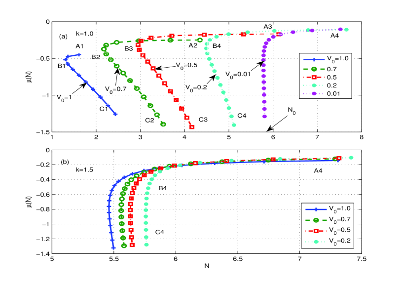
Figure 1: (Color online) Chemical potential $\mu$ of the ground-state mode (“soliton”) versus its norm $N$, at two fixed wavenumbers of the Penrose-tiling potential, $k=1$ (a) and $k=1.5$ (b), and different values of its depth, $V_{0}$. Labels $Cj$ and $Aj$ ($j=1,2,3,4$) indicate VK-stable and unstable branches, respectively, while points $Bj$ mark junctions between them.

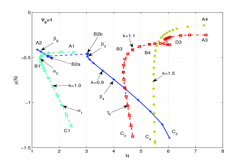
Figure 2: (Color online) The same as in Fig. 1, but for the fixed depth of the OL potential, and different values of its wavenumber.

As said above, the main point in this work is the study of the solitons close to norm-minimizing points $\mathrm{Bj}$, which are of obvious interest to the potential experiment. In Fig. 1 we observe that stable solitons with the minimum norm (i.e., smallest number of atoms) are, naturally, generated in the deepest potential, represented by families $\mathrm{A1-B1-C1}$. The norm attains its minimum, $N_{\min}=1.304$ (with $\mu=-0.518$) at $k=1$ and $V_{0}=1$ [point $\mathrm{B1}$ in Fig. 1(a)]. We also observe that the stability range (the distance from the lower termination point to point $\mathrm{B1}$) in Fig. 1(a) for $k=1$ is $\Delta N=N(\mathrm{C1})-N(\mathrm{B1})=2.531-1.304=\allowbreak 1.\,\allowbreak 227$, which is $\simeq 20$ times larger than $\Delta N=5.510-5.460=\allowbreak 0.05$  in Fig. 1(b) for $k=1.5$, at the same OL depth, $V_{0}=1$. Generally, the comparison of Fig. 1(a) and Fig. 1(b) demonstrates that, for given $V_{0}$, the norm of the ground states strongly depends on the OL wavenumber, $k$.

The branch $\mu(N)$ with $k=0.9$ in Fig. 2 is notably different from other branches with $k\geq 1$. Although a continuous dependence $\mu(N)$ is found in the range of $\mathrm{C2-B2b}$, no solutions have been found (the imaginary-time algorithm does not converge to them) between points $\mathrm{B2b}$ and $\mathrm{B2a}$ (the dashed segment $\mathrm{B2b-B2a}$ is depicted in Fig. 2 only as a guide to the eye). The algorithm again converges to the ground-state modes in the range of $\mathrm{B2a-A2}$.

Furthermore, a tail of segment $\mathrm{B2b-C2}$ of this branch penetrates into the overcritical region, $N=6.046>N_{\mathrm{Townes}}=5.85$. This feature is explained by the fact that the solitons found at $k\leq 0.9$ (in particular, the ones marked by $\beta_{3},\beta_{4},\beta_{6}$ in Fig. 2) are actually double-humped structures, featuring pairs of spatially separated or almost fused density peaks [see Figs. 4(c) and 5(a), respectively].

Stability of the solitons. The VK criterion does not guarantee the full stability of solitons, as it does not capture instabilities associated with complex eigenvalues. To test the full stability, we simulated perturbed evolution of the solitons over a sufficiently long interval, typically $t=1000$ (which covers, roughly, $10$ diffraction times of the corresponding localized states), adding small random perturbation to the initial conditions, with a relative amplitude $\sim 0.01$. The modes whose evolution was tested in this way are indicated by arrows in Fig. 2, attached to symbols $\alpha_{1},\alpha_{2}$ and $\beta_{3},\beta_{4},\beta_{6}$, which pertain to branches with $k=1$ and $k=0.9$, respectively, and $\gamma_{5}$, that pertains to $k=1.1$. The results of the evolution simulations are shown in Figs. 3-5.

Figure 3 presents details of the stability test for the ground state on branch $\mathrm{C1}$, marked by $\alpha_{1}$ in Fig. 2 (for $V_{0}=1$ and $k=1$), with the norm and chemical potential $N=2.098$ and $\mu=-1.027$. This mode is stable. 

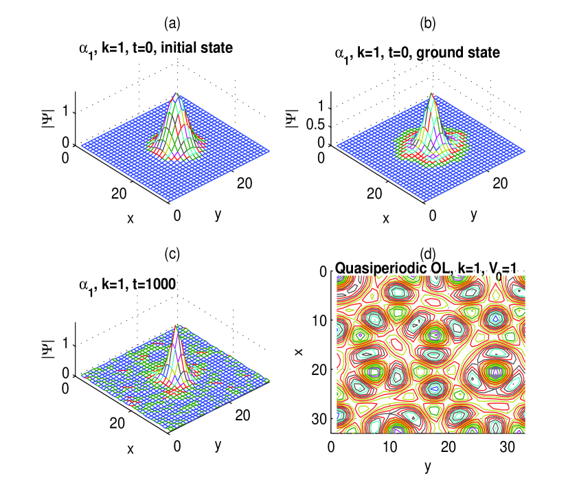
Figure 3: (Color online.) The spatial structure of the stable localized mode supported by the quasiperiodic potential, labeled by $\alpha_{1}$ in Fig. 2. (a) The Gaussian initial configuration (3) for $V_{0}=1$ and $k=1$, transformed by the imaginary-time relaxation into the ground state, which is shown in panel (b). Panel (c): The result of the perturbed evolution (in real time) at $t=1000$. (d) The contour-plot profile of the underlying quasiperiodic potential with $V_{0}=1$ and $k=1.0$.

Figures 4 (a) and (b) display the evolution of the solitons taken near the junction points between the VK-stable and unstable segments of the $\mu(N)$ curves, for $k=1$ and $k=0.9$. Figure 4(a) pertains to the mode labeled $\alpha_{2}$ (with $k=1$) in Fig. 2, which evolves into the perturbed state depicted at $t=200$ in Fig. 4(b). This mode is unstable, splitting into a set of density peaks located at different potential minima, which, however, do not tend to decay into dispersive waves. The evolution of another unstable mode, labeled by $\beta_{6}$ in Fig. 2, is displayed in Figs. 4(c) and 4(d). It splits into two parts, and eventually decays into the dispersive radiation either.

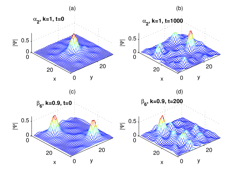
Figure 4: (Color online) The evolution of the stationary modes labeled by points $\alpha_{2}$ and $\beta_{6}$ in Fig. 2, for $k=0.9$ and $V_{0}=1$. (a) The shape of mode $\alpha_{2}$, with $N=1.304$, $\mu=-0.518$; (b) the result of the evolution at $t=1000$. The final state is not a bound one, but it does not decay into radiation. (c,d) Mode $\beta_{6}$ with $N=1.319$, $\mu=-0.434$, which splits into two parts, and eventually decays.

Finally, Fig. 5 represents the perturbed evolution of the mode with larger norms ($N>4$), for $k=0.9$ and $k=1.1$, which correspond to points $\beta_{4}$ and $\gamma_{5}$, respectively, labeled in Fig. 2. In panels 5(a,b) we again observe that the former (double-peak) mode, corresponding to $k=0.9$, does not produce a stable soliton in the course of the perturbed evolution. However, Fig. 5(d) demonstrates that the soliton corresponding to point $\gamma_{5}$ is stable. The eventual conclusion following from the analysis of the numerical results is that all the double-peak structures are unstable against splitting, irrespective of their formal compliance with the VK criterion, while the single-peak solitons are stable or not in the exact accordance with VK.

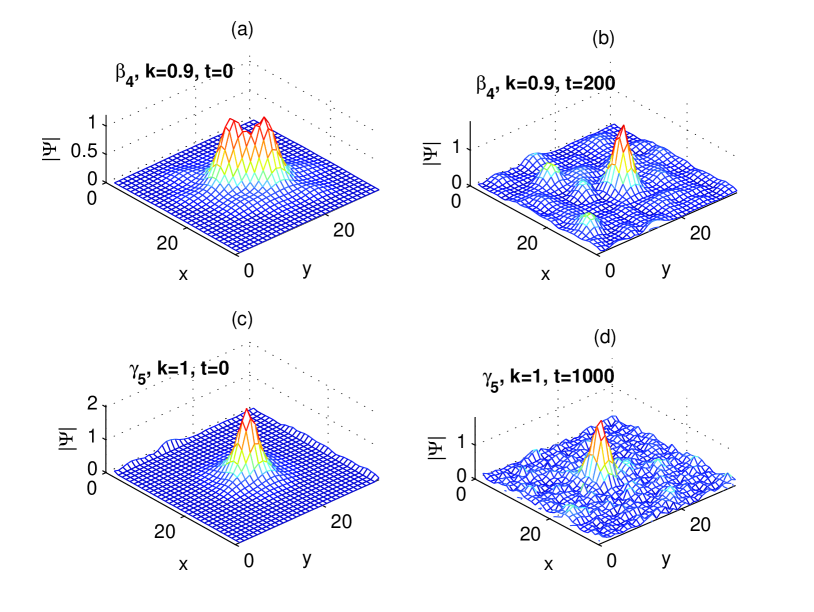
Figure 5: (Color online) The perturbed evolution of modes $\beta_{4}$ (a,b) and $\gamma_{5}$ (c,d), which are marked in Fig. 2). The former one, with $N=4.002$ and $\mu=-0.743$, is unstable, while the latter mode ($\gamma_{5}$), with $N=4.510$ and $\mu=-1.035$, is stable.

Conclusion. We have studied the dynamics of 2D matter-wave solitons near the junction points between the stable and unstable branches of curves $\mu(N)$ for the soliton families supported by the interplay of the self-attractive nonlinearity and Penrose-tiling OL potential. These points are interesting to physical applications, as they correspond to the smallest number of atoms which is necessary to build 2D matter-wave solitons, or the smallest total power necessary for the making of spatial optical solitons. It was found that the shape and stability of such solitons crucially depend on the depth and period of the OL. A challenging problem is to extend the analysis to vortex solitons supported by quasi-periodic potentialsBBB3 .

This work was supported, in a part, by CONACyT/SEP 2012 and PROMEP CA Redes projects (México).

References

- (1) B. A. Malomed, D. Mihalache, F. Wise, and L. Torner, J. Optics B: Quant. Semics. Opt. 7, R53 (2005).
- (2) F. Lederer, G. I. Stegeman, D. N. Christodoulides, G. Assanto, M. Segev, and Y. Silberberg, Phys. Rep. 463, 1 (2008).
- (3) Y. V. Kartashov, B. A. Malomed, and L. Torner, Rev. Mod. Phys. 83, 247 (2011).
- (4) B. B. Baizakov, B. A. Malomed, and M. Salerno, Europhys. Lett. 63, 642 (2003); J. Yang and Z. H. Musslimani, Opt. Lett. 28, 2094 (2003); Z. H. Musslimani and J. Yang, J. Opt. Soc. Am. B 21, 973 (2004).
- (5) B. B. Baizakov, B. A. Malomed and M. Salerno, Phys. Rev. A 70, 053613 (2004); Eur. Phys. J. D 38, 367 (2006); T. Mayteevarunyoo, B. A. Malomed, B. B. Baizakov, and M. Salerno, Physica D 238, 1439 (2009).
- (6) B. B. Baizakov, B. A. Malomed and M. Salerno, in: Nonlinear Waves: Classical and Quantum Aspects, ed. by F. Kh. Abdullaev and V. V. Konotop, p. 61 (Kluwer Academic Publishers: Dordrecht, 2004).
- (7) D. Goldberg, L. I. Deych, A. A. Lisyansky, Z. Shi, V. M. Menon, V. Tokranov, M. Yakimov, and S. Oktyabrsky, Nature Photonics 3, 662 (2009); D. Bajoni, D. Gerace, M. Galli, J. Bloch, R. Braive, I. Sagnes, A. Miard, A. Lemaitre, M. Patrini, and L. C. Andreani, Phys. Rev. B 80, 201308 (2009); ): E. A. Cerda-Mendez, D. N. Krizhanovskii, M. Wouters, R. Bradley, K. Biermann, K. Guda, R. Hey, P. V. Santos, D. Sarkar, and M. S. Skolnick, Phys. Rev. Lett. 105, 116402 (2010); N. Y. Kim, K. Kusudo, C. J. Wu, N. Masumoto, A. Loffler, S. Hofling, N. Kumada, L. Worschech, A. Forchel, and Y. Yamamoto, Nature Physics 7, 681 (2011).
- (8) J. Kasprzak, M. Richard, S. Kundermann, A. Baas, P. Jeambrun, J. M. J. Keeling, F. M. Marchetti, M. H. Szymanska, R. Andre, J. L. Staehli, V. Savona, P. B. Littlewood, B. Deveaud, and L. S. Dang, Nature 443, 409 (2006).
- (9) T. C. H. Liew, I. A. Shelykh, and G. Malpuech, Physica E 43, 1543 (2011).
- (10) D. Mihalache, D. Mazilu, F. Lederer, Y. V. Kartashov, L.-C. Crasovan, and L. Torner, Phys. Rev. E 70, 055603(R) (2004).
- (11) H. L. F. da Luz, F. Kh. Abdullaev, A. Gammal, M. Salerno, and L. Tomio, Phys. Rev. A 82, 043618 (2010).
- (12) B. A. Malomed, Soliton Management in Periodic Systems (Springer, New York, 2006).
- (13) F. Kh. Abdullaev, J. G. Caputo, R. A. Kraenkel, and B. A. Malomed, Phys. Rev. A 67, 013605 (2003); H. Saito and M. Ueda , Phys. Rev. Lett. 90, 040403 (2003); G. D. Montesinos, V. M. Pérez-García, and H. Michinel, Phys. Rev. Lett. 92, 133901 (2004); A. Itin, T. Morishita, and S. Watanabe, Phys. Rev. A 74, 033613 (2006).
- (14) P. G. Kevrekidis, G. Theocharis, D. J. Frantzeskakis, and B.A. Malomed, Phys. Rev. Lett. 90, 230401 (2003); D. E. Pelinovsky, P. G. Kevrekidis, and D. J. Frantzeskakis, ibid. 91, 240201 (2003); F. Kh. Abdullaev, R. M. Galimzyanov, M. Brtka, and R. A Kraenkel, J. Phys. B: At. Mol. Opt. Phys. 37, 3535 (2004).
- (15) M. Matuszewski, E. Infeld, B. A. Malomed, and M. Trippenbach, Phys. Rev. Lett. 95, 050403 (2005).
- (16) J. J. Garcia-Ripoll and V. M. Pérez-García, Phys. Rev. A 59, 2220 (1999); J. J. García-Ripoll, V. M. Pérez-García, and Pedro Torres, Phys. Rev. Lett. 83, 1715 (1999); M. Krämer, C. Tozzo, and F. Dalfovo, Phys. Rev. A 71, 061602(R) (2005); B. Baizakov, G. Filatrella, B. Malomed, and M. Salerno, Phys. Rev. E 71, 036619 (2005); C. Tozzo, M. Krämer, and F. Dalfovo, Phys. Rev. A 72, 023613 (2005); P. Engels, C. Atherton, and M. A. Hoefer, Phys. Rev. Lett. 98, 095301 (2007); Yu. Kagan and L. A. Manakova, Phys. Rev. A 76, 023601 (2007).
- (17) I. Towers and B. A. Malomed, J. Opt. Soc. Am. 19, 537 (2002).
- (18) M. Centurion, M. A. Porter, P. G. Kevrekidis, and D. Psaltis, Phys. Rev. Lett. 97, 033903 (2006).
- (19) G. D. Montesinos, V. M. Pérez-García, and H. Michinel, Phys. Rev. Lett. 92, 133901 (2004); J. Abdullaev, D. Poletti, E. Ostrovskaya, and Yu. S. Kivshar, ibid. 105, 090401 (2010).
- (20) G. Burlak and B. A. Malomed, Phys. Rev. A 77, 053606 (2008).
- (21) P. Pedri and L. Santos, Phys. Rev. Lett. 95, 200404 (2005); I. Tikhonenkov, B. A. Malomed, and A. Vardi, ibid. 100, 090406 (2008).
- (22) D. Briedis, D. E. Petersen, D. Edmundson, W. Królikowski, and O. Bang, Opt. Exp. 13, 435 (2005); S. Lopez-Aguayo, A. S. Desyatnikov, Y. S. Kivshar, S. Skupin, W. Królikowski, and O. Bang, Opt. Lett. 31, 1100 (2006); D. Buccoliero, A. S. Desyatnikov, W. Królikowski, and Y. S. Kivshar, Phys. Rev. Lett. 98, 053901 (2007); S. Skupin. M. Saffman, and W. Królikowski, ibid. 98, 263902 (2007); V. M. Lashkin, A. I. Yakimenko, and O. O. Prikhodko, Phys. Lett. A 366, 422 (2007).
- (23) G. Roati, C. D’Errico, L. Fallani, M. Fattori, C. Fort, M. Zaccanti, G. Modugno, M. Modugno, and M. Inguscio, Nature 453, 895 (2008); L. Fallani, C. Fort, and M. Inguscio, in: Adv. At. Mol. Opt. Phys. 56, 119 (2008) (ed. by E. Arimondo P. R. Berman, and C. C. Lin); S. K. Adhikari and L. Salasnich, Phys. Rev. A 80, 023606 (2009); M. Larcher, F. Dalfovo, and M. Modugno, Phys. Rev. A 80, 053606 (2009).
- (24) H. Sakaguchi, B. A. Malomed, Phys. Rev. E 74, 026601 (2006).
- (25) G. Burlak and A. Klimov, Phys. Lett. A 369, 510 (2007).
- (26) K. E. Strecker, G. B. Partridge, A. G. Truscott, and F. G. Hulet, Nature 417, 150 (2002); L. Khaykovich, F. Schreck, G. Ferrari, T. Bourdel, J. Cubizolles, L. D. Carr, Y. Castin, and C. Salomon, Science 296, 1290 (2002); S. L. Cornish, S. T. Thompson, and C. E. Wieman, Phys. Rev. Lett. 96, 170401 (2006).
- (27) N. G. Vakhitov and A. A. Kolokolov, Izv. Vys. Uch. Zaved., Radiofizika 16, 1020 (1973) [in Russian; English translation: Radiophys. Quant. Electr. 16, 783 (1975)].
- (28) L. Bergé, Phys. Rep. 303, 259 (1998); E. A. Kuznetsov and F. Dias, Phys. Rep. 507, 43 (2011).
- (29) B. B. Baizakov and M. Salerno, Phys. Rev. A 69, 013602 (2004).
- (30) F. Dalfovo, S. Giorgini, and L. P. Pitaevskii, Rev. Mod. Phys. 71, 463 (1999).
- (31) J. Yang and T. I. Lakoba, Stud. Appl. Math. 120, 265 (2008).