Quantum Hydrodynamic Model by Moment Closure of Wigner Equation

Abstract

In this paper, we derive the quantum hydrodynamics models based on the moment closure of the Wigner equation. The moment expansion adopted is of the Grad type firstly proposed in [18]. The Grad’s moment method was originally developed for the Boltzmann equation. In [7], a regularization method for the Grad’s moment system of the Boltzmann equation was proposed to achieve the globally hyperbolicity so that the local well-posedness of the moment system is attained. With the moment expansion of the Wigner function, the drift term in the Wigner equation has exactly the same moment representation as in the Boltzmann equation, thus the regularization in [7] applies. The moment expansion of the nonlocal Wigner potential term in the Wigner equation is turned to be a linear source term, which can only induce very mild growth of the solution. As the result, the local well-posedness of the regularized moment system for the Wigner equation remains as for the Boltzmann equation.

Keywords: Moment closure; Wigner equation; Boltzmann equation; quantum hydrodynamics

1 Introduction

The Wigner equation was proposed by Wigner in 1932 as a counterpart in quantum mechanics of the Boltzmann equation [37]. Different from the distribution function in the Boltzmann equation, the Wigner function may take negative values, so it is not a true probability distribution function. But it is called a “quasi-probability distribution function” in the phase space because it allows one to express quantum mechanical averages (related to statistical moments) in a form which is very similar to that for classical averages. Readers may refer to the review article by Hillery et al. [20] for more details of the properties of the Wigner function. It offers a convenient interpretation of the ensemble in the form of a quasi-probability distribution in the phase space defined by position $\boldsymbol{x}$ and momentum $\boldsymbol{p}$ and has been proved to of great use not only as a calculation tools but can also provide insights into the connections between classical and quantum mechanical mechanics. Actually, Lions et al. have given a rigorous mathematical proof that in the semiclassical limit, the Wigner equation gives the Vlasov (or Liouville) equation in the phase space [28]. As one of the most accurate equations in quantum mechanics, the Wigner equation has many advantages over the Schrödinger equation, the nonequilibrium Green method and the density matrix method in simulating the carrier transport in semiconductor devices because the description of boundary conditions and collision operator for the semi-classical Boltzmann equation can be extended to the Wigner equation due to their strong similarity [14]. There has been an increasing interest in the Wigner equation as the size of semiconductor devices goes into the nano-scale under which the quantum effects becomes not negligible any more [13]. In some devices, the quantum effect even plays a dominating role, e.g., the resonant tunneling diode (RTD) has been extensively studied recently using the numerical methods based on the Wigner equation [15]. The numerical method for the Wigner equations has attracted many researchers from different fields [31, 17, 29, 25, 22, 26, 38, 5]. The deterministic numerical methods have been successfully used in simulating one-dimensional devices, but are not expected to be directly used for multi-dimensional devices simulation due to its formidable expense in memory storage and computational time. One practical approach to investigate a higher dimensional devices where quantum effects are relevant is to use quantum hydrodynamics models which are moment systems derived from the Wigner equation. Because the close connection of the Wigner equation and the Boltzmann equation, many moment methods devised for the Boltzmann equation have been extended to the Wigner equation, see [16, 12] and references therein. Equations derived from the Wigner equation are called quantum drift-diffusion equations, quantum Euler equations and quantum hydrodynamics equation, and numerical simulations based on such moment equations are extensively studied [39, 11, 24, 21]. In this paper, we will extended the moment method recently proposed in [7] for the Boltzmann equation to the Wigner equation.

In 1940s, Grad [18] proposed a moment method to approximate the Boltzmann equation, and a 13-moment model is given as an extension of the classic Euler equations. However, this model was quickly found to be problematic [19]. Its major deficiencies include the appearance of subshocks in the structure of a strong shock wave and the loss of global hyperbolicity. Later on, a number of regularizations were raised to solve or alleviate these problems. Levermore [27] introduced a promising way to achieve global hyperbolicity, while 14 moments are needed and the explicit expressions of the equations cannot be written. Jin and Slemrod [23] gave a regularization of the Burnett equations via relaxation, which resulted in a set of equations containing the same variables with Grad’s 13-moment theory, and no subshocks appear in the structure of shock waves. Struchtrup and Torrilhon [33] regularized Grad’s system by integrating the moment method with Chapman-Enskog expansion, and the resulting system is called as the R13 equations. And in [32], Struchtrup improved the R13 equations by the “order of magnitude” method. The R13 system also removes the discontinuities in the shock wave, and it extends the region of hyperbolicity considerably [34]. Recently, Torrilhon [35] tackled the problem of hyperbolicity by introducing the Pearson-Type-IV distributions, and the resulting system is proven to be able to gain a much larger hyperbolicity region.

Due to the complexity of the explicit expressions, systems with large number of moments are not investigated until recently. In [36], Torrilhon and his coworkers developed a software named $ET_{XX}$ [2] which is able to generate moment systems with almost any number of moments in one-dimensional space. And in [3], some numerical results for a shock tube were carried out to show the behavior of characteristic waves in the extended thermodynamics. A numerical method solving large moment systems was proposed in [8], and therein the regularization technique in [33] was applied to general moment systems. In [10], the order of magnitude method was also integrated into large moment systems. In [6], the authors focused on the one-dimensional velocity space, and the characteristic polynomial of the quasi-linear coefficient matrix is found to be very simple; thus a brand-new regularized model with global hyperbolicity is proposed by the correction of the characteristic speed. Such regularization is extended to the multi-dimensional velocity space in [7].

It is clear that the moment expansion of the drift term for Boltzmann equation can be extended to the Wigner equation. The resulting convective terms in the moment system expanded from the drift term of the Wigner equation has exactly the same format as that of the Boltzmann equation. Thus the method of the hyperbolic regularization in [7] is applied to the Wigner equation, too, to achieve the global hyperbolicity. As the difference of the Wigner equation from the Boltzmann equation, the nonlocal Wigner potential term due to the electric potential is also expanded using Hermite polynomial. It is interesting for us to find that this term can be represented in the moment expansion style with very compact expressions. The overall formation of the nonlocal Wigner potential term in the moments is turned into a linear source term, with compact sparse coefficient matrix. Moreover, the contribution from the lower order moments in this term is always on the higher order moments. Immediately, the coefficient matrix in the linear source term is strictly lower triangular, thus it is a nilponent matrix. Noticing that the moment expansion of the relaxation scattering term produces a linear source term providing an exponential decay of the high order moments. As a result, the growth of the high order moments in time due to the source term is essentially slower than exponential growth rate. This makes that the derived moment system is formulated as a quasi-linear system, plus a linear source term which can induce only very mild growth of the high order moments. Since the convection term in the system is guaranteed to be globally hyperbolic by the regularization, the local well-posedness of the system is out of box.

The rest of this paper is arranged as follows: in Section 2 we present the elementary formula of Wigner equation. The moment expansion of Wigner equation is carried out in Section 3 and the system obtained is closed by truncation of the expansion and regularized using method in [7] in Section 4 to achieve the final hyperbolic system. In Section 5, we discuss the simple case in 1D space for better understanding of the structure of the derived moment system. Concluding remarks are in the last section.

2 Wigner Equation with Smooth Potential

We consider a one-particle system in a statistical mixture with $N$ states described by the wave functions $\Psi_{k}=\Psi_{k}(t,\boldsymbol{x})$, each with a probability $P_{k}\geqslant 0$, with $k=1,\cdots,N_{\text{state}}$, which satisfies $\sum_{k=1}^{N_{\text{state}}}P_{k}=1$. The wave functions $\Psi_{k}(t,\boldsymbol{x})$ of state $k$ obeys the Schrödinger equation

$$i\hbar\dfrac{\partial{\Psi_{k}(t,\boldsymbol{x})}}{\partial{t}}=-\frac{\hbar^{2}}{2m}\nabla_{\boldsymbol{x}}^{2}\Psi_{k}(t,\boldsymbol{x})+V(t,\boldsymbol{x})\Psi_{k}(t,\boldsymbol{x}),$$ (1)

where $i=\sqrt{-1}$, $\hbar$ is the reduced Planck constant, $m$ is the particle effective mass assumed to a constant in this paper, and $V(t,\boldsymbol{x})$ is the electric potential energy (which will be called potential for short hereafter). We can also regard the one-particle system as a many-particle system with $P_{k}$ interpreted as the percentage of the particles occupying state $k$. This is the general way the Wigner equation used in modeling carrier transport in semiconductor devices. We construct the Wigner function $f(t,\boldsymbol{x},\boldsymbol{p})$ which is a quasi-probability density function in the phase space $(\boldsymbol{x},\boldsymbol{p})$, as usual, by

$$f(t,\boldsymbol{x},\boldsymbol{p})=\frac{1}{(2\pi\hbar)^{3}}\sum_{k=1}^{N_{\text{state}}}P_{k}\int_{\mathbb{R}^{3}}\Psi_{k}^{*}(t,\boldsymbol{x}+\boldsymbol{y}/2)\Psi_{k}(t,\boldsymbol{x}-\boldsymbol{y}/2)e^{i\boldsymbol{y}\cdot\boldsymbol{p}/\hbar}d^{3}\boldsymbol{y}.$$ (2)

Using the Schrödinger equation (1) and the definition of the Wigner function given above, we can derive the Wigner equation (or the quantum Vlasov equation) as been done in [37, 20]

$$\dfrac{\partial{f}}{\partial{t}}+\frac{\boldsymbol{p}}{m}\cdot\nabla_{\boldsymbol{x}}f+\Theta[V]f=0,\quad\boldsymbol{x}\in\mathbb{R}^{3},\ \boldsymbol{p}\in\mathbb{R}^{3},$$ (3)

where the nonlocal Wigner potential term $\Theta[V]f$ is a pseudo-differential operator. It is defined by

$$(\Theta[V]f)(t,\boldsymbol{x},\boldsymbol{p})=\int_{\mathbb{R}^{3}}V_{w}(t,\boldsymbol{x},\boldsymbol{p}^{\prime})f(t,\boldsymbol{x},\boldsymbol{p}-\boldsymbol{p}^{\prime})\,\mathrm{d}\boldsymbol{p}^{\prime},$$ (4)

where the Wigner potential is as

$$V_{w}(t,\boldsymbol{x},\boldsymbol{p})=\frac{-i}{(2\pi\hbar)^{3}\hbar}\int_{\mathbb{R}^{3}}\left[V\left(t,\boldsymbol{x}+\frac{\boldsymbol{y}}{2}\right)-V\left(t,\boldsymbol{x}-\frac{\boldsymbol{y}}{2}\right)\right]e^{i\boldsymbol{y}\cdot\boldsymbol{p}/\hbar}\,\mathrm{d}\boldsymbol{y}.$$

For convenience, we simply take $m=1$ later on. Similar to a Vlasov-Poisson system, a Wigner-Poisson system could be also considered to include the self-consistent electric field induced by the redistribution of the electrons. In this paper, we focus on the case that $V(t,\boldsymbol{x})$ is a given smooth function. The pseudo-operator $\Theta[V]f$ can be written into an equivalent form [20]

$$(\Theta[V]f)(t,\boldsymbol{x},\boldsymbol{p})=-\sum_{\boldsymbol{\lambda}}\frac{(\hbar/2i)^{|{\boldsymbol{\lambda}}|-1}}{{\boldsymbol{\lambda}}!}\frac{\partial^{{\boldsymbol{\lambda}}}V}{\partial\boldsymbol{x}^{{\boldsymbol{\lambda}}}}\frac{\partial^{{\boldsymbol{\lambda}}}f}{\partial\boldsymbol{p}^{{\boldsymbol{\lambda}}}},$$ (5)

where ${\boldsymbol{\lambda}}=(\lambda_{1},\lambda_{2},\lambda_{3})$, $|{\boldsymbol{\lambda}}|=\sum_{i=1}^{3}\lambda_{i}$, $\boldsymbol{x}^{{\boldsymbol{\lambda}}}=\prod_{i=1}^{3}x_{i}^{\lambda_{i}}$,

$$\dfrac{\partial^{\boldsymbol{\lambda}}}{\partial\boldsymbol{x}^{\boldsymbol{\lambda}}}=\prod_{i=1}^{3}\dfrac{\partial^{\lambda_{i}}}{\partial x_{i}^{\lambda_{i}}},\qquad\dfrac{\partial^{\boldsymbol{\lambda}}}{\partial\boldsymbol{p}^{\boldsymbol{\lambda}}}=\prod_{i=1}^{3}\dfrac{\partial^{\lambda_{i}}}{\partial p_{i}^{\lambda_{i}}},$$

and the summation over ${\boldsymbol{\lambda}}$ has to be extended over all non-negative integer values of $\lambda_{1},\lambda_{2},\lambda_{3}$ for which $|{\boldsymbol{\lambda}}|$ is odd. In the semi-classical limit $\hbar\rightarrow 0$, $\Theta[V]f$ converges to the usual operator $-\nabla_{\boldsymbol{x}}V\cdot\nabla_{\boldsymbol{p}}f$. The equation (3) describes particles movement without scattering corresponding to ballistic transport. The scattering effect may be considered by adding a scattering term to the right hand side of (3). So one obtains the following Wigner equation with a scattering term:

$$\dfrac{\partial{f}}{\partial{t}}+\boldsymbol{p}\cdot\nabla_{\boldsymbol{x}}f+\Theta[V]f=\left.\dfrac{\partial{f}}{\partial{t}}\right|_{\mathrm{Scat}},\quad\boldsymbol{x}\in\mathbb{R}^{3},\ \boldsymbol{p}\in\mathbb{R}^{3}.$$ (6)

The time-relaxation approximation of the scattering term is often used for the Wigner equation [15], and it has the same form of the BGK scattering term used for the collision of gas [4]. It is easy to be study analytically and takes of the following simple form

$$\left.\dfrac{\partial{f}}{\partial{t}}\right|_{\mathrm{Scat}}=\frac{f_{\mathrm{eq}}-f}{\tau},$$ (7)

where $\tau$ is the relaxation time and $f_{\mathrm{eq}}$ is the equilibrium distribution. For example, when the density of electrons are not extremely high, we can assume that the equilibrium distribution is a Maxwellian distribution,

$$f_{\mathrm{eq}}(t,\boldsymbol{x},\boldsymbol{p})=\frac{\rho(t,\boldsymbol{x})}{\left(2\pi k_{B}T\right)^{3/2}}\exp\left(-\frac{(\boldsymbol{p}-\boldsymbol{u}(t,x))^{2}}{2k_{B}T(t,\boldsymbol{x})}\right)$$ (8)

where $\rho(t,\boldsymbol{x})$ is the number density of particles at position $\boldsymbol{x}$, $k_{B}$ is the Boltzmann constant, $T(t,\boldsymbol{x})$ is the particle temperature, and $\boldsymbol{u}(t,\boldsymbol{x})$ is the average momentum of particles. These macroscopic variables are related with the distribution function as below:

$$\rho(t,\boldsymbol{x})=\int_{\mathbb{R}^{3}}f(t,\boldsymbol{x},\boldsymbol{p})\,\mathrm{d}\boldsymbol{p},$$ (9)

$$\rho(t,\boldsymbol{x})\boldsymbol{u}(t,\boldsymbol{x})=\int_{\mathbb{R}^{3}}\boldsymbol{p}f(t,\boldsymbol{x},\boldsymbol{p})\,\mathrm{d}\boldsymbol{p},$$ (10)

$$\rho(t,\boldsymbol{x})k_{B}T(t,\boldsymbol{x})=\int_{\mathbb{R}^{3}}|\boldsymbol{p}-\boldsymbol{u}|^{2}f(t,\boldsymbol{x},\boldsymbol{p})\,\mathrm{d}\boldsymbol{p}.$$ (11)

The conservation of mass, momentum and total energy are all valid for the Wigner equation. Multiplying the equation (6) by $1$ and $\boldsymbol{p}$, direct integration with $\boldsymbol{p}$ and $\boldsymbol{x}$ gives us

$$\frac{\,\mathrm{d}}{\,\mathrm{d}t}\int_{\mathbb{R}^{3}\times\mathbb{R}^{3}}f(t,\boldsymbol{x},\boldsymbol{p})\,\mathrm{d}\boldsymbol{x}\,\mathrm{d}\boldsymbol{p}=0,\quad t\in\mathbb{R}^{+},$$ (12)

$$\frac{\,\mathrm{d}}{\,\mathrm{d}t}\int_{\mathbb{R}^{3}\times\mathbb{R}^{3}}\boldsymbol{p}f(t,\boldsymbol{x},\boldsymbol{p})\,\mathrm{d}\boldsymbol{x}\,\mathrm{d}\boldsymbol{p}=-\int_{\mathbb{R}^{3}}\rho(t,\boldsymbol{x})\dfrac{\partial{V(t,\boldsymbol{x})}}{\partial{\boldsymbol{x}}}\,\mathrm{d}\boldsymbol{x},\quad t\in\mathbb{R}^{+}.$$ (13)

Multiplying the equation (6) by $|\boldsymbol{p}|^{2}$ and integrating by parts, we get the conservation of the total energy for the system (6) and (5):

$$\frac{\,\mathrm{d}}{\,\mathrm{d}t}\int_{\mathbb{R}^{3}\times\mathbb{R}^{3}}f(t,\boldsymbol{x},\boldsymbol{p})|\boldsymbol{p}|^{2}\,\mathrm{d}\boldsymbol{x}\,\mathrm{d}\boldsymbol{p}=-2\int_{\mathbb{R}^{3}}\rho(t,\boldsymbol{x})\boldsymbol{u}(t,\boldsymbol{x})\cdot\nabla_{\boldsymbol{x}}V(t,\boldsymbol{x})\,\mathrm{d}\boldsymbol{x},\quad t\in\mathbb{R}^{+}.$$ (14)

3 Grad Moment System

In this section, we derive the moment system of the Wigner equation using the Grad type moment expansion.

3.1 Hermite expansion of the distribution function

Following the method in [8, 10], we expand the distribution function into Hermite series as

$$f(t,\boldsymbol{x},\boldsymbol{p})=\sum_{\alpha\in\mathbb{N}^{3}}f_{\alpha}(t,\boldsymbol{x})\mathcal{H}_{\mathcal{T},\alpha}\left(\frac{\boldsymbol{p}-\boldsymbol{u}(t,\boldsymbol{x})}{\sqrt{\mathcal{T}(t,\boldsymbol{x})}}\right),$$ (15)

where $\alpha=(\alpha_{1},\alpha_{2},\alpha_{3})$ is a three-dimensional multi-index. The basis functions $\mathcal{H}_{\mathcal{T},\alpha}$ are the 3-dimensional Hermite functions defined by

$$\mathcal{H}_{\mathcal{T},\alpha}(\boldsymbol{\xi})=\prod\limits_{d=1}^{3}\frac{1}{\sqrt{2\pi}}\mathcal{T}^{-\frac{\alpha_{d}+1}{2}}\mathit{He}_{\alpha_{d}}(\xi_{d})\exp\left(-\frac{\xi_{d}^{2}}{2}\right),$$ (16)

where $\mathit{He}_{n}(x)$ is the Hermite polynomial of order $n$

$$\mathit{He}_{n}(x)=(-1)^{n}\exp\left(\frac{x^{2}}{2}\right)\frac{\,\mathrm{d}^{n}}{\,\mathrm{d}x^{n}}\exp\left(-\frac{x^{2}}{2}\right).$$ (17)

For convenience, $\mathit{He}_{n}(x)$ is taken as zero if $n<0$, thus $\mathcal{H}_{\mathcal{T},\alpha}(\boldsymbol{\xi})$ is zero when any component of $\alpha$ is negative. The parameter $\mathcal{T}$ in the expansion is the scaled local temperature as

$$\mathcal{T}(t,\boldsymbol{x})=k_{B}T(t,\boldsymbol{x}).$$ (18)

It is clear that the equilibrium distribution $f_{\mathrm{eq}}$ is coincidently equal to the first term of expansion, i.e.,

$$f_{\mathrm{eq}}(t,\boldsymbol{x},\boldsymbol{p})=f_{0}(t,\boldsymbol{x})\mathcal{H}_{\mathcal{T},0}\left(\frac{\boldsymbol{p}-\boldsymbol{u}(t,\boldsymbol{x})}{\sqrt{\mathcal{T}(t,\boldsymbol{x})}}\right),$$ (19)

where $f_{0}(t,\boldsymbol{x})=\rho(t,\boldsymbol{x})$. So in this case the relaxation time approximation scattering term (20) can be written as the linear combination of the basis functions of orders greater than or equal to $1$,

$$\frac{1}{\tau}(f_{M}-f)=-\frac{1}{\tau}\sum_{|\alpha|\geq 1}f_{\alpha}\mathcal{H}_{\mathcal{T},\alpha}\left(\frac{\boldsymbol{p}-\boldsymbol{u}(t,\boldsymbol{x})}{\sqrt{\mathcal{T}(t,\boldsymbol{x})}}\right).$$ (20)

The definition of the Hermite function (16) shows that each basis function is an exponentially decaying function multiplied by a multi-dimensional Hermite polynomial shifted by the local macroscopic momentum $\boldsymbol{u}$ and scaled by the square root of the local temperature $\mathcal{T}$.

If one uses arbitrary known function $\boldsymbol{u}^{\prime}(t,\boldsymbol{x})$ and $\mathcal{T}^{\prime}(t,\boldsymbol{x})$ in (15) to expand the distribution function $f(t,\boldsymbol{x},\boldsymbol{p})$ as

$$f(t,\boldsymbol{x},\boldsymbol{p})=\sum_{\alpha\in\mathbb{N}^{3}}f_{\alpha}^{\prime}(t,\boldsymbol{x})\mathcal{H}_{\mathcal{T}^{\prime},\alpha}\left(\frac{\boldsymbol{p}-\boldsymbol{u}^{\prime}(t,\boldsymbol{x})}{\sqrt{\mathcal{T}^{\prime}(t,\boldsymbol{x})}}\right),$$ (21)

then the following relations between the macroscopic quantities $\boldsymbol{u}$, $\mathcal{T}$, the coefficients $f_{\alpha}$, and $\boldsymbol{u}^{\prime}$, $\mathcal{T}^{\prime}$, the coefficients $f_{\alpha}^{\prime}$ can be derived as follows,

$$\rho =f_{0}=f_{0}^{\prime},$$ (22a)

$$\rho\boldsymbol{u} =\rho\boldsymbol{u}^{\prime}+(f_{e_{d}}^{\prime})_{d=1,2,3}^{T},$$ (22b)

$$\rho|\boldsymbol{u}-\boldsymbol{u}^{\prime}|^{2}+3\rho\mathcal{T} =\sum\limits_{d=1}^{3}(\mathcal{T}^{\prime}f_{0}^{\prime}+2f_{2e_{d}}^{\prime}),$$ (22c)

where $e_{d}$ is the unit vector with its $d$-th entry to be $1$. It is clear that the coefficients $f_{\alpha}$ expanded using parameters $\boldsymbol{u}$ and $\mathcal{T}$ satisfy the following conditions:

$$f_{e_{i}}=0,\quad\sum\limits_{d=1}^{3}f_{2e_{d}}=0,\quad i=1,2,3.$$ (23)

Moreover, if we define the heat flux $q_{i}$ and the pressure tensor $P=\{p_{ij}\},\ i,j=1,2,3$ with

$$q_{i}=\frac{1}{2}\int_{\mathbb{R}^{3}}|\boldsymbol{p}-\boldsymbol{u}|^{2}(p_{i}-u_{i})f\,\mathrm{d}\boldsymbol{p},$$ (24)

$$p_{ij}=\int_{\mathbb{R}^{3}}(p_{i}-u_{i})(p_{j}-u_{j})f\,\mathrm{d}\boldsymbol{p},$$ (25)

then direct calculations give us the relations between them and the coefficients $f_{\alpha}$ in (15) as

$$q_{i}=2f_{3e_{i}}+\sum_{d=1}^{3}f_{2e_{d}+e_{i}},$$ (26)

$$p_{ij}-\frac{1}{3}\delta_{ij}\sum_{d=1}^{3}p_{dd}=(1+\delta_{ij})f_{e_{i}+e_{j}}.$$ (27)

By the definition of the temperature (11) and (18) and the definition of the tensor pressure (27), the scaled temperature $\mathcal{T}$ is a linear combination of $p_{ij}$ as

$$\rho\mathcal{T}=\dfrac{1}{3}\sum_{d=1}^{3}p_{dd}.$$ (28)

With the relation (27), we then have

$$p_{ij}=\delta_{ij}\rho\mathcal{T}+(1+\delta_{ij})f_{e_{i}+e_{j}}.$$ (29)

3.2 Moment expansion of the Wigner equation

Now we are ready to derive the moment system by taking the moments of the Wigner equation. The general method to get the moment system is to first multiply the Wigner equation (6) of by polynomials of momentum $\boldsymbol{p}$ of different order and then integrate both sides over momentum $\boldsymbol{p}$ on $\mathbb{R}^{3}$. One equivalent way is as follows. First, we substitute the expansion of the Wigner function (15) into the Wigner equation (6), then we collect the coefficients of basis functions of the same order at both sides, and finally we equate the coefficients of the basis functions of the same order on both sides to yield the derived moment system. We plug the Hermite series (15) into the Wigner equation (6), and make calculations by noting that the Hermite function (16) used in this paper depends also on the time $t$ and position $\boldsymbol{x}$ through $\boldsymbol{u}(t,\boldsymbol{x})$ and $\mathcal{T}(t,\boldsymbol{x})$, which is different from the general expansion using the Hermite functions depending only on the momentum $\boldsymbol{p}$ [30]. For convenience, we list some useful relations of Hermite polynomials as below [1]:

1. Orthogonality: $\displaystyle\int_{\mathbb{R}}\mathit{He}_{l}(x)\mathit{He}_{n}(x)\exp(-x^{2}/2)\,\mathrm{d}x=l!\sqrt{2\pi}\delta_{l,n}$;

2. Recursion relation: $\mathit{He}_{n+1}(x)=x\mathit{He}_{n}(x)-n\mathit{He}_{n-1}(x)$;

3. Differential relation: $\mathit{He}_{n}^{\prime}(x)=n\mathit{He}_{n-1}(x)$.

And the following equality can be derived from the last two relations:

$$[\mathit{He}_{n}(x)\exp(-x^{2}/2)]^{\prime}=-\mathit{He}_{n+1}(x)\exp(-x^{2}/2).$$ (30)

Especially, we have

$$\dfrac{\partial{}}{\partial{p_{j}}}{\mathcal{H}_{\mathcal{T},\alpha}\left(\frac{\boldsymbol{p}-\boldsymbol{u}}{\sqrt{\mathcal{T}}}\right)}=-\mathcal{H}_{\mathcal{T},\alpha+e_{j}}\left(\frac{\boldsymbol{p}-\boldsymbol{u}}{\sqrt{\mathcal{T}}}\right).$$ (31)

With these relations, the part

$$\dfrac{\partial{f}}{\partial{t}}+\boldsymbol{p}\cdot\nabla_{\boldsymbol{x}}f$$

of (6) is expanded as

$$\begin{split}&~{}~{}\sum_{\alpha\in\mathbb{N}^{3}}\Bigg{\{}\left(\frac{\partial f_{\alpha}}{\partial t}+\sum_{d=1}^{3}\frac{\partial u_{d}}{\partial t}f_{\alpha-e_{d}}+\frac{1}{2}\frac{\partial\mathcal{T}}{\partial t}\sum_{d=1}^{3}f_{\alpha-2e_{d}}\right)\\ &\qquad+\sum_{j=1}^{3}\Bigg{[}\left(\mathcal{T}\frac{\partial f_{\alpha-e_{j}}}{\partial x_{j}}+u_{j}\frac{\partial f_{\alpha}}{\partial x_{j}}+(\alpha_{j}+1)\frac{\partial f_{\alpha+e_{j}}}{\partial x_{j}}\right)\\ &\qquad\qquad+\sum_{d=1}^{3}\frac{\partial u_{d}}{\partial x_{j}}\left(\mathcal{T}f_{\alpha-e_{d}-e_{j}}+u_{j}f_{\alpha-e_{d}}+(\alpha_{j}+1)f_{\alpha-e_{d}+e_{j}}\right)\\ &\qquad\qquad+\frac{1}{2}\frac{\partial\mathcal{T}}{\partial x_{j}}\sum_{d=1}^{3}\left(\mathcal{T}f_{\alpha-2e_{d}-e_{j}}+u_{j}f_{\alpha-2e_{d}}+(\alpha_{j}+1)f_{\alpha-2e_{d}+e_{j}}\right)\Bigg{]}\Bigg{\}}\mathcal{H}_{\mathcal{T},\alpha}\left(\frac{\boldsymbol{p}-\boldsymbol{u}}{\sqrt{\mathcal{T}}}\right).\end{split}$$ (32)

Then using (31), we calculate the pseudo-operator term $\Theta[V]f$ expressed in (5), and obtain

$$(\Theta[V]f)(t,\boldsymbol{x},\boldsymbol{p})=\sum_{\alpha,{\boldsymbol{\lambda}}}\frac{(\hbar/2i)^{|{\boldsymbol{\lambda}}|-1}}{{\boldsymbol{\lambda}}!}\frac{\partial^{{\boldsymbol{\lambda}}}V}{\partial\boldsymbol{x}^{{\boldsymbol{\lambda}}}}f_{\alpha-{\boldsymbol{\lambda}}}\mathcal{H}_{\mathcal{T},\alpha}\left(\frac{\boldsymbol{p}-\boldsymbol{u}}{\sqrt{\mathcal{T}}}\right),$$ (33)

where the summation over ${\boldsymbol{\lambda}}$ means the same as that in (5), and $f_{\alpha-{\boldsymbol{\lambda}}}$ is taken as zero when any component of $\alpha-{\boldsymbol{\lambda}}$ is negative. Finally, the scattering term $\left.\dfrac{\partial{f}}{\partial{t}}\right|_{\mathrm{Scat}}$ given in (8) becomes

$$-\frac{1}{\tau}\sum_{|\alpha|\geq 2}f_{\alpha}\mathcal{H}_{\mathcal{T},\alpha}\left(\frac{\boldsymbol{p}-\boldsymbol{u}}{\sqrt{\mathcal{T}}}\right),$$ (34)

noticing that $f_{e_{d}}=0$, $d=1,2,3$.

Collecting the three terms (32), (33) and (34) yielded after the substitution of the Hermite expansion (15) into the Wigner equation (6), we can get the following general moment equations with a slight rearrangement by matching the coefficients of the same weight function:

$$\begin{split}&\frac{\partial f_{\alpha}}{\partial t}+\sum_{d=1}^{3}\left(\frac{\partial u_{d}}{\partial t}+\sum_{j=1}^{3}u_{j}\frac{\partial u_{d}}{\partial x_{j}}\right)f_{\alpha-e_{d}}+\frac{1}{2}\left(\frac{\partial\mathcal{T}}{\partial t}+\sum_{j=1}^{3}u_{j}\frac{\partial\mathcal{T}}{\partial x_{j}}\right)\sum_{d=1}^{3}f_{\alpha-2e_{d}}\\ &\qquad\qquad+\sum_{j,d=1}^{3}\Big{[}\frac{\partial u_{d}}{\partial x_{j}}\left(\mathcal{T}f_{\alpha-e_{d}-e_{j}}+(\alpha_{j}+1)f_{\alpha-e_{d}+e_{j}}\right)\\ &\qquad\qquad+\frac{1}{2}\frac{\partial\mathcal{T}}{\partial x_{j}}\left(\mathcal{T}f_{\alpha-2e_{d}-e_{j}}+(\alpha_{j}+1)f_{\alpha-2e_{d}+e_{j}}\right)\Big{]}\\ &\qquad\qquad+\sum_{j=1}^{3}\left(\mathcal{T}\frac{\partial f_{\alpha-e_{j}}}{\partial x_{j}}+u_{j}\frac{\partial f_{\alpha}}{\partial x_{j}}+(\alpha_{j}+1)\frac{\partial f_{\alpha+e_{j}}}{\partial x_{j}}\right)\\ &\qquad\qquad=-\frac{1}{\tau}\mathrm{H}(|\alpha|-2)f_{\alpha}-\sum_{{\boldsymbol{\lambda}}}\frac{(\hbar/2i)^{|{\boldsymbol{\lambda}}|-1}}{{\boldsymbol{\lambda}}!}\frac{\partial^{{\boldsymbol{\lambda}}}V}{\partial\boldsymbol{x}^{{\boldsymbol{\lambda}}}}f_{\alpha-{\boldsymbol{\lambda}}},\end{split}$$ (35)

where $\mathrm{H}(x)$ is the Heaviside function defined by

$$\mathrm{H}(x)=\left\{\begin{array}[]{ll}0,&\text{if}~{}~{}x<0,\\ 1,&\text{if}~{}~{}x\geqslant 0.\end{array}\right.$$ (36)

By setting $\alpha=0$ in (35), we deduce the mass conservation

$$\dfrac{\partial{\rho}}{\partial{t}}+\sum_{j=1}^{3}\left(u_{j}\dfrac{\partial{\rho}}{\partial{x_{j}}}+\rho\dfrac{\partial{u_{j}}}{\partial{x_{j}}}\right)=0.$$ (37)

By setting $\alpha=e_{d}$, with $d=1,2,3$ and noting that $f_{e_{d}}=0$ in (35), we obtain

$$\rho\left(\dfrac{\partial{u_{d}}}{\partial{t}}+\sum_{j=1}^{3}u_{j}\dfrac{\partial{u_{d}}}{\partial{x_{j}}}\right)+\rho\dfrac{\partial{\mathcal{T}}}{\partial{x_{d}}}+\mathcal{T}\dfrac{\partial{\rho}}{\partial{x_{d}}}+\sum_{j=1}^{3}(\delta_{jd}+1)\dfrac{\partial{f_{e_{d}+e_{j}}}}{\partial{x_{j}}}=-\rho\dfrac{\partial{V}}{\partial{x_{d}}},$$ (38)

which is simplified as

$$\rho\left(\dfrac{\partial{u_{d}}}{\partial{t}}+\sum_{j=1}^{3}u_{j}\dfrac{\partial{u_{d}}}{\partial{x_{j}}}\right)+\sum_{j=1}^{3}\dfrac{\partial{p_{jd}}}{\partial{x_{j}}}=-\rho\dfrac{\partial{V}}{\partial{x_{d}}}.$$ (39)

By setting $\alpha=2e_{d}$, with $d=1,2,3$ and noting that $f_{e_{d}}=0$, we obtain

$$\begin{split}\dfrac{\partial{f_{2e_{d}}}}{\partial{t}}&+\frac{\rho}{2}\left(\dfrac{\partial{\mathcal{T}}}{\partial{t}}+\sum_{j=1}^{3}u_{j}\dfrac{\partial{\mathcal{T}}}{\partial{x_{j}}}\right)+\rho\mathcal{T}\dfrac{\partial{u_{d}}}{\partial{x_{d}}}+\sum_{j,l}(1+\alpha_{j})f_{2e_{d}-e_{l}+e_{j}}\dfrac{\partial{u_{l}}}{\partial{x_{j}}}\\ &\qquad\qquad\qquad\qquad+\sum_{j=1}^{3}u_{j}\dfrac{\partial{f_{2e_{d}}}}{\partial{x_{j}}}+(1+2\delta_{jd})\dfrac{\partial{f_{2e_{d}+e_{j}}}}{\partial{x_{j}}}=-\frac{1}{\tau}f_{2e_{d}}.\end{split}$$ (40)

Noting that $\sum_{d=1}^{3}f_{2e_{d}}=0$, we sum the upper equations over $d$ to get

$$\rho\left(\dfrac{\partial{\mathcal{T}}}{\partial{t}}+\sum_{j=1}^{3}u_{j}\dfrac{\partial{\mathcal{T}}}{\partial{x_{j}}}\right)+\frac{2}{3}\sum_{j=1}^{3}\left(\dfrac{\partial{q_{j}}}{\partial{x_{j}}}+\sum_{d=1}^{3}p_{jd}\dfrac{\partial{u_{d}}}{\partial{x_{j}}}\right)=0.$$ (41)

Since $\rho\mathcal{T}=\frac{1}{3}\sum_{d=1}^{3}p_{dd}$, we have

$$\dfrac{\partial{\mathcal{T}}}{\partial{x_{j}}}=\frac{1}{3\rho}\sum_{d=1}^{3}\dfrac{\partial{p_{dd}}}{\partial{x_{j}}}-\frac{\mathcal{T}}{\rho}\dfrac{\partial{\rho}}{\partial{x_{j}}},\quad j=1,2,3.$$ (42)

Substituting (39), (41) and (42) into (35), we eliminate the time derivatives of $\boldsymbol{u}$ and $\mathcal{T}$ and the spatial derivatives of $\mathcal{T}$. Then the quasi-linear form of the moment system reads:

$$\begin{split}&\dfrac{\partial{f_{\alpha}}}{\partial{t}}+\sum_{j=1}^{3}\left(\mathcal{T}\dfrac{\partial{f_{\alpha-e_{j}}}}{\partial{x_{j}}}+u_{j}\dfrac{\partial{f_{\alpha}}}{\partial{x_{j}}}+(\alpha_{j}+1)\dfrac{\partial{f_{\alpha+e_{j}}}}{\partial{x_{j}}}\right)\\ &\qquad+\sum_{j=1}^{3}\sum_{d=1}^{3}\dfrac{\partial{u_{d}}}{\partial{x_{j}}}\left(\mathcal{T}f_{\alpha-e_{d}-e_{j}}+(\alpha_{j}+1)f_{\alpha-e_{d}+e_{j}}-\frac{p_{jd}}{3\rho}\sum_{k=1}^{3}f_{\alpha-2e_{k}}\right)\\ &\qquad-\sum_{j=1}^{3}\sum_{d=1}^{3}\frac{f_{\alpha-e_{d}}}{\rho}\dfrac{\partial{p_{jd}}}{\partial{x_{j}}}-\frac{1}{3\rho}\left(\sum_{k=1}^{3}f_{\alpha-2e_{k}}\right)\sum_{j=1}^{3}\dfrac{\partial{q_{j}}}{\partial{x_{j}}}\\ &\qquad+\sum_{j=1}^{3}\left(\left(-\frac{\mathcal{T}}{2\rho}\dfrac{\partial{\rho}}{\partial{x_{j}}}+\frac{1}{6\rho}\sum_{d=1}^{3}\dfrac{\partial{p_{dd}}}{\partial{x_{j}}}\right)\sum_{k=1}^{3}\left(\mathcal{T}f_{\alpha-2e_{k}-e_{j}}+(\alpha_{j}+1)f_{\alpha-2e_{k}+e_{j}}\right)\right)\\ &\qquad=-\frac{1}{\tau}\mathrm{H}(|\alpha|-2)f_{\alpha}-\sum_{{\boldsymbol{\lambda}}}\frac{(\hbar/2i)^{|{\boldsymbol{\lambda}}|-1}}{{\boldsymbol{\lambda}}!}\dfrac{\partial{{}^{{\boldsymbol{\lambda}}}V}}{\partial{\boldsymbol{x}^{{\boldsymbol{\lambda}}}}}f_{\alpha-{\boldsymbol{\lambda}}},\qquad\forall~{}|\alpha|\geq 2.\end{split}$$ (43)

We should point out again the summation over ${\boldsymbol{\lambda}}$ is extended over all the non-negative integers $\lambda_{d}$, $d=1,2,3$ for which $|{\boldsymbol{\lambda}}|$ is odd and greater than $1$. Especially for $|\alpha|\leq 2$, the moment system (43) derived from the Wigner equation is the same as that derived from the Boltzmann equation [9].

With (29), we can have the equations for $p_{ij}$ by (43). Precisely, we have the equation for $p_{ii}/2$, $i=1,2,3$, as

$$\begin{split}\dfrac{\partial{p_{ii}/2}}{\partial{t}}&+\sum_{j=1}^{3}u_{j}\dfrac{\partial{p_{ii}/2}}{\partial{x_{j}}}+\sum_{j=1}^{3}\left(\frac{1}{2}+\delta_{ij}\right)\rho\mathcal{T}\dfrac{\partial{u_{j}}}{\partial{x_{j}}}+\sum_{j=1}^{3}\sum_{d=1}^{3}(2\delta_{ij}+1)f_{2e_{i}-e_{d}+e_{j}}\dfrac{\partial{u_{d}}}{\partial{x_{j}}}\\ &\qquad\qquad+\sum_{j=1}^{3}(2\delta_{ij}+1)\dfrac{\partial{f_{2e_{i}+e_{j}}}}{\partial{x_{j}}}=-\frac{1}{2\tau}\left(p_{ii}-\frac{1}{3}\sum_{d=1}^{3}p_{dd}\right),\quad i=1,2,3.\end{split}$$ (44)

If $i\neq j$, we have $p_{ij}=f_{e_{i}+e_{j}}$, thus its equation is already in (43).

We collect the equations (37), (39), (44) and (43) together to obtain a moment system with infinite number of equations. Noting that the relation between $u_{d}$ and $f_{e_{d}}$ given in (22) and the definition of $q_{i}$ and of $p_{ij}$ given in (27), we can see that what we obtain is a quasi-linear system for $f_{\alpha}$. We would like to point out that the only difference between the system derived from the Wigner equation and that from the Boltzmann equation is the term with high-order derivatives of the potential $V(t,\boldsymbol{x})$, which is a source term of the quasi-linear system of $f_{\alpha}$.

4 Moment Closure with Global Hyperbolicity

The moment system derived from the Wigner equation consists of (37), (39), (44) and (43). It is clear that this is a system with infinite number of equations taken $\rho$, $u_{d}$, $p_{ij}$ and $f_{\alpha}$, $|\alpha|\geqslant 3$, as unknowns. To obtain a system with finite unknowns, we will truncate the expansion (15) and close the system following the method in [7].

With a truncation of (15), (43) will result in a finite moment system. Precisely, we let $M\geqslant 3$ be a positive integer and only the coefficients in the set $\mathcal{M}=\{f_{\alpha}\}_{|\alpha|\leqslant M}$ are considered. Let $F_{M}(\boldsymbol{u},\mathcal{T})$ denotes the linear space spanned by all $\mathcal{H}_{\mathcal{T},\alpha}\left(\frac{\boldsymbol{p}-\boldsymbol{u}(t,\boldsymbol{x})}{\sqrt{\mathcal{T}(t,\boldsymbol{x})}}\right)$’s with $|\alpha|\leqslant M$, and the expansion (15) is truncated as

$$f(t,\boldsymbol{x},\boldsymbol{p})\approx\sum_{|\alpha|\leqslant M}f_{\alpha}(t,\boldsymbol{x})\mathcal{H}_{\mathcal{T},\alpha}\left(\frac{\boldsymbol{p}-\boldsymbol{u}(t,\boldsymbol{x})}{\sqrt{\mathcal{T}(t,\boldsymbol{x})}}\right),$$ (45)

with $f(t,\boldsymbol{x},\boldsymbol{p})\in F_{M}(\boldsymbol{u},\mathcal{T})$ and $f_{\alpha}\in\mathcal{M}$. The moment equations which contain $\partial{f_{\alpha}}/\partial{t}$ with $|\alpha|>M$ are disregarded in (43). Then, (37), (39), (44) and (43) with $2\leqslant|\alpha|\leqslant M$ lead to a system with finite number of equations.

Following [7], we let

$${\cal{S}}_{M}=\{\alpha\in\mathbb{N}^{3}\mid|\alpha|\leq M\}.$$

Then for any $\alpha\in{\cal{S}}_{M}$, let

$${\mathcal{N}}(\alpha)=\sum_{i=1}^{3}\binom{\sum_{k=4-i}^{3}\alpha_{k}+i-1}{i}+1$$ (46)

to be the ordinal number of $\alpha$ in ${\cal{S}}_{M}$, and the cardinal number of set ${\cal{S}}_{M}$ is

$$N={\mathcal{N}}(Me_{3})=\binom{M+3}{3},$$

which is total number of moments if a truncation with $|\alpha|\leq M$ is applied.

Let $\boldsymbol{w}=(w_{1},\cdots,w_{N})^{T}\in\mathbb{R}^{N}$ and for each $i,j\in\{1,2,3\}$ and $i\neq j$,

$$w_{1} =\rho, w_{{\mathcal{N}}(e_{i})} =u_{i},$$ (47a)

$$w_{{\mathcal{N}}(2e_{i})} =\frac{p_{ii}}{2}, w_{{\mathcal{N}}(e_{i}+e_{j})} =p_{ij},$$ (47b)

$$w_{{\mathcal{N}}(\alpha)} =f_{\alpha},\quad 3\leq|\alpha|\leq M.$$ (47c)

The moment system (37), (39), (44) and (43) is collected in quasi-linear format as

$$\dfrac{\partial{\boldsymbol{w}}}{\partial{t}}+\sum_{j=1}^{3}{\bf M}_{j}(\boldsymbol{w})\dfrac{\partial{\boldsymbol{w}}}{\partial{x_{j}}}={\bf G}\boldsymbol{w},$$ (48)

by taking the derivatives of $f_{\alpha+e_{j}}$, $|\alpha|=M$ to be zero, where ${\bf M}_{j}$ and ${\bf G}$ are $N\times N$ matrices. The entries of ${\bf M}_{j}$ are given as the coefficients of the terms in (37), (39), (44) and (43) with derivatives of $\boldsymbol{w}$. The entries of ${\bf G}$ arise from the nonlocal Wigner potential term and the scattering term. From (44), one can observe that

$${\bf G}_{{\mathcal{N}}(2e_{i}),{\mathcal{N}}(2e_{j})}=-\frac{1}{\tau}(\delta_{ij}-\frac{1}{3}),\quad i,j=1,2,3.$$ (49)

And (43) indicates that the diagonal entries of the lower right part of ${\bf G}$ are

$${\bf G}_{{\mathcal{N}}(\alpha),{\mathcal{N}}(\alpha)}=-\frac{1}{\tau}\mathrm{H}(|\alpha|-2),\quad\text{ for }|\alpha|\geq 2\text{ and }\alpha\neq 2e_{i},~{}~{}i=1,2,3.$$ (50)

From (39), it is clear that

$${\bf G}_{{\mathcal{N}}(e_{i}),1}=-\dfrac{1}{\rho}\dfrac{\partial{V}}{\partial{x_{i}}},\quad i=1,2,3.$$ (51)

The other nonzero entries of ${\bf G}$ from the nonlocal Wigner potential are as

$${\bf G}_{{\mathcal{N}}(\alpha),{\mathcal{N}}(\alpha-{\boldsymbol{\lambda}})}=-\frac{(\hbar/2i)^{|{\boldsymbol{\lambda}}|-1}}{{\boldsymbol{\lambda}}!}\frac{\partial^{{\boldsymbol{\lambda}}}V}{\partial\boldsymbol{x}^{{\boldsymbol{\lambda}}}},$$ (52)

where $|{\boldsymbol{\lambda}}|$ is odd and $|{\boldsymbol{\lambda}}|$ is greater than $1$ and $|\alpha-{\boldsymbol{\lambda}}|\neq 1$ or $2$. In case of $|\alpha-{\boldsymbol{\lambda}}|=1$, we have ${\bf G}_{{\mathcal{N}}(\alpha),{\mathcal{N}}(\alpha-{\boldsymbol{\lambda}})}=0$ since $f_{e_{i}}=0$, $i=1,2,3$. In case of $|\alpha-{\boldsymbol{\lambda}}|=2$, we have (52) if $\alpha-{\boldsymbol{\lambda}}=e_{i}+e_{j}$, $i\neq j$, since $w_{{\mathcal{N}}(e_{i}+e_{j})}=p_{ij}=f_{e_{i}+e_{j}}$. The difference is in case of $\alpha-{\boldsymbol{\lambda}}=2e_{i}$, $i=1,2,3$. Precisely by (29), we have

$${\bf G}_{{\mathcal{N}}(\alpha),{\mathcal{N}}(2e_{i})}=-\sum_{j=1}^{3}\left(\delta_{ij}-\dfrac{1}{3}\right)\frac{(\hbar/2i)^{|\alpha|-3}}{(\alpha-2e_{j})!}\frac{\partial^{\alpha-2e_{j}}V}{\partial\boldsymbol{x}^{\alpha-2e_{j}}}.$$ (53)

All other entries of ${\bf G}$ vanishes except for the ones specified above. It is clear that the non-zero entries defined by (49) and (50) by the scattering term provide us a linear damping of the high order moment. The contribution of the nonlocal Wigner potential matrix ${\bf G}$ is strictly lower triangular. Thus these part of the matrix is nilponent. As a result, the growth of the high order moments in time due to the nonlocal Wigner potential term is essentially slower than exponential growth rate.

In (48), we following Grad [18] take ${\partial f_{\alpha+e_{j}}}/{\partial x_{j}}$, $|\alpha|=M$, as zero to make the system to be closed. It has been pointed out in [7] that it is not appropriate to set $\partial f_{\alpha+e_{j}}/\partial x_{j}=0$, $|\alpha|=M$, as the closure proposed in [18] since the system is lack of hyperbolicity if the distribution function is far away from the equilibrium. To obtain a system with global hyperbolicity, we have to adopt the regularization given in [7]. For any $\alpha$ with $|\alpha|=M$, we define

$${\cal R}_{M}^{j}(\alpha)=(\alpha_{j}+1)\left[\sum_{d=1}^{3}f_{\alpha-e_{d}+e_{j}}\dfrac{\partial{u_{d}}}{\partial{x_{j}}}+\frac{1}{2}\left(\sum_{d=1}^{3}f_{\alpha-2e_{d}+e_{j}}\right)\dfrac{\partial{\mathcal{T}}}{\partial{x_{j}}}\right].$$ (54)

and

$$\hat{\bf M}_{j}\dfrac{\partial{\boldsymbol{w}}}{\partial{x_{j}}}={\bf M}_{j}\dfrac{\partial{\boldsymbol{w}}}{\partial{x_{j}}}-\sum_{|\alpha|=M}{\cal R}_{M}^{j}(\alpha)I_{{\mathcal{N}}(\alpha)},\quad\text{ for any admissible }\boldsymbol{w},$$ (55)

where $I_{k}$ is the $k$-th column of the $N\times N$ identity matrix. We regularize the system (48) as

$$\dfrac{\partial{\boldsymbol{w}}}{\partial{t}}+\sum_{j=1}^{3}\hat{\bf M}_{j}(\boldsymbol{w})\dfrac{\partial{\boldsymbol{w}}}{\partial{x_{j}}}={\bf G}\boldsymbol{w},$$ (56)

which is the quantum hydrodynamics model we derived. It has been proved in [7] that

Theorem 1.

The regularized moment system (56) is hyperbolic for any $\boldsymbol{w}$ with positive temperature. Precisely, for a given unit vector $\boldsymbol{n}=(n_{1},n_{2},n_{3})$, the matrix

$$\sum_{j=1}^{3}n_{j}\hat{\bf M}_{j}(\boldsymbol{w})$$ (57)

is diagonalizable with eigenvalues as

$$\boldsymbol{u}\cdot\boldsymbol{n}+{\rm{C}}_{{n},{m}}\sqrt{\mathcal{T}},\qquad 1\leqslant n\leqslant m\leqslant M+1,$$ (58)

where ${\rm{C}}_{{n},{m}}$ is a root of $m$-order Hermite polynomial, and satisfies ${\rm{C}}_{{1},{m}}<\cdots<{\rm{C}}_{{m},{m}}$. The structure of the $N$ eigenvectors can be fully clarified.

Based on this theorem, the regularized moment system (56) is locally well-posed due to the hyperbolicity. We would like to mention here that the regularization here actually does not add any new terms to the system (48). On the contrary, it has erased the terms in (43) with a factor $\alpha_{j}+1$ in its coefficient for the equations of $f_{\alpha}$ with $|\alpha|=M$ only.

5 Regularized Moment System in 1D

In 1D space, the structure of the system we derived is significantly simpler than in multi-dimensional case. In this section, we give the detailed formation of the moment system in 1D case since the 1D Wigner equation is already very useful in modelling of RTDs [15].

The 1D Wigner equation is as

$$\dfrac{\partial{f}}{\partial{t}}+p\dfrac{\partial{f}}{\partial{x}}-\sum_{\lambda=1,3,5,\cdots}\frac{(\hbar/2i)^{\lambda-1}}{\lambda!}\dfrac{\partial{{}^{\lambda}V}}{\partial{x^{\lambda}}}\dfrac{\partial{{}^{\lambda}f}}{\partial{p^{\lambda}}}=\frac{1}{\tau}(f_{\mathrm{eq}}-f),$$ (59)

where effective mass is again assumed to be $1$ for convinence. The equilibrium distribution $f_{\mathrm{eq}}$ is assumed to be a 1D Maxwellian distribution

$$f_{\mathrm{eq}}(t,x,p)=\frac{\rho(t,x)}{\sqrt{2\pi k_{B}T}}\exp\left(-\frac{(p-u(t,x))^{2}}{2k_{B}T(t,x)}\right).$$ (60)

The 1D Wigner function is expanded as

$$f(t,x,p)=\sum_{n\in\mathbb{N}}f_{n}(t,x,p)\mathcal{H}_{\mathcal{T},n}\left(\frac{p-u}{\sqrt{\mathcal{T}}}\right),$$ (61)

where

$$\mathcal{H}_{\mathcal{T},n}(x)=\frac{1}{\sqrt{2\pi}}\mathcal{T}^{-(n+1)/2}\mathit{He}_{n}(x)\exp(-x^{2}/2),$$ (62)

and the 1D density $\rho$ and average momentum $u$ are defined by

$$\rho=\int_{-\infty}^{\infty}f(t,x,p)dp,\quad u=\frac{1}{\rho}\int_{-\infty}^{\infty}pf(t,x,p)dp,$$ (63)

and the scaled temperature $\mathcal{T}$ defined by

$$\mathcal{T}=k_{B}T=\frac{1}{\rho}\int_{-\infty}^{\infty}(p-u)^{2}f(t,x,p)dp.$$ (64)

The above equation plus the definition for the pressure (25) for $P$ shows that

$$P=\rho\mathcal{T}.$$ (65)

In one dimension, (23) becomes

$$f_{1}=0,\quad f_{2}=0.$$ (66)

The relation (26) between the heat flux $q$ and the coefficient $f_{3}$ of the expansion is turned to be

$$q=3f_{3}.$$ (67)

We present below the details of the regularized moment system truncated at very low order based on (56), though the closed moment system up to any order can be written in a general formation. We will demonstrate that with the low order expansions of the distribution function, the moment system obtained is able to capture very typical quantum effects. As the simplest case, a closed regularized moment system truncated up to $M=3$ is

$$\dfrac{\partial{\rho}}{\partial{t}}+u\dfrac{\partial{\rho}}{\partial{x}}+\rho\dfrac{\partial{u}}{\partial{x}}=0,$$ (68)

$$\rho\dfrac{\partial{u}}{\partial{t}}+\rho u\dfrac{\partial{u}}{\partial{x}}+\dfrac{\partial{P}}{\partial{x}}=-\dfrac{\partial{V}}{\partial{x}}\rho,$$ (69)

$$\dfrac{\partial{P/2}}{\partial{t}}+u\dfrac{\partial{P/2}}{\partial{x}}+\dfrac{3}{2}P\dfrac{\partial{u}}{\partial{x}}+3\dfrac{\partial{f_{3}}}{\partial{x}}=0.$$ (70)

$$\dfrac{\partial{f_{3}}}{\partial{t}}-\dfrac{P^{2}}{2\rho^{2}}\dfrac{\partial{\rho}}{\partial{x}}+\dfrac{P}{2\rho}\dfrac{\partial{P}}{\partial{x}}+u\dfrac{\partial{f_{3}}}{\partial{x}}=-\dfrac{1}{\tau}f_{3}+\dfrac{\hbar^{2}}{24}\dfrac{\partial{{}^{3}V}}{\partial{x^{3}}}\rho,$$ (71)

where $\dfrac{\hbar^{2}}{24}\dfrac{\partial{{}^{3}V}}{\partial{x^{3}}}\rho$ is the quantum correction term yielded by the nonlocal Wigner potential. We reformulate (68), (69), (70), (71) into a matrix form

$$\dfrac{\partial{\boldsymbol{w}}}{\partial{t}}+{\bf M}(\boldsymbol{w})\dfrac{\partial{\boldsymbol{w}}}{\partial{x}}={\bf G}{\boldsymbol{w}},$$ (72)

where $\boldsymbol{w}=\left(\rho,u,P/2,f_{3}\right)^{T}$ and

$${\bf M}=\begin{pmatrix}u&\rho&0&0\\ 0&u&\dfrac{2}{\rho}&0\\ 0&3P&u&3\\ -\dfrac{P^{2}}{2\rho^{2}}&0&\dfrac{P}{\rho}&u\end{pmatrix},$$ (73)

$${\bf G}=\begin{pmatrix}0&0&0&0\\ -\dfrac{\partial{V}}{\partial{x}}\dfrac{1}{\rho}&0&0&0\\ 0&0&0&0\\ \dfrac{\hbar^{2}}{24}\dfrac{\partial{{}^{3}V}}{\partial{x^{3}}}&0&0&-\dfrac{1}{\tau}\end{pmatrix}.$$ (74)

Here we consider the following example to show the difference between the quantum moment system and the classical moment system. The Boltzmann equation in 1D with a potential

$$V(x)=\left\{\begin{array}[]{ll}\exp\left(-\frac{1}{1-x^{2}}\right),&\text{if}\ \ |x|<1,\\ 0,&\text{else},\end{array}\right.$$ (75)

admits a steady solution

$$f(t,x,p)=\frac{1}{\sqrt{2\pi}}\exp\left(-\frac{p^{2}}{2}-V(x)\right),$$ (76)

with its moments as

$$\rho=P=\exp(-V(x)),\quad u=f_{3}=0.$$ (77)

$\rho$, $u$, $P$ and $f_{3}$ in (77) satisfy the moment system derived from the Boltzmann equation which can be obtained from (72) by removing the term $-\dfrac{\hbar^{2}}{24}\dfrac{\partial{{}^{3}V}}{\partial{x^{3}}}\rho$. The solutions given in (77) show that the classical behavior of particles obeys the Newtons law, i.e., the particles with low kinetic energy ($p^{2}/2$ at position $x$ ) can not move to a new position with energy $V(x^{\prime})$ which is greater than $p^{2}/2+V(x)$. As a result, $\rho$ in (77) will not change in time.

In the quantum mechanics, the particles behave like a wave that the particles with lower energy can be tunneled through a potential barrier. The moment system derived from the Wigner equation will reflect this point. Let us consider the system (72) with (77) as initial value. We carry out an asymptotic analysis to study the behavior of the solution around $t=0$, using time $t$ as the asymptotic expansion parameter. The ansatz we adopted is as

$$f_{3} =f_{3,0}+f_{3,1}t+\mathcal{O}(t^{2}),$$ (78)

$$P =P_{0}+P_{1}t+P_{2}t^{2}+\mathcal{O}(t^{3}),$$ (79)

$$u =u_{0}+u_{1}t+u_{2}t^{2}+u_{3}t^{3}+\mathcal{O}(t^{4}),$$ (80)

$$\rho =\rho_{0}+\rho_{1}t+\rho_{2}t^{2}+\rho_{3}t^{3}+\rho_{4}t^{4}+\mathcal{O}(t^{5}),$$ (81)

where the leading order terms are as the initial value

$$\rho_{0}=P_{0}=\exp(-V(x)),\quad u_{0}=f_{3,0}=0.$$ (82)

Substituting the ansatz into (71), we immediately have

$$f_{3,1}=\frac{\hbar^{2}}{24}V^{(3)}(x)\rho_{0},$$ (83)

thus $f_{3}$ is as

$$f_{3}=\frac{\hbar^{2}}{24}V^{\left(3\right)}(x)\rho_{0}t+\mathcal{O}(t^{2})$$ (84)

Plugging (84) and (79) - (81) into (70), we obtain

$$P_{1}=0,\quad P_{2}=-\frac{\hbar^{2}}{24}\dfrac{\,\mathrm{d}{}}{\,\mathrm{d}{x}}\left(V^{\left(3\right)}(x)\rho_{0}\right),$$ (85)

which yields

$$P=P_{0}-\frac{\hbar^{2}}{8}\dfrac{\,\mathrm{d}{}}{\,\mathrm{d}{x}}\left(V^{\left(3\right)}(x)\rho_{0}\right)t^{2}+\mathcal{O}(t^{3}).$$ (86)

Similar procedure gives us

$$u=u_{0}+\frac{\hbar^{2}}{24}\dfrac{\,\mathrm{d}{{}^{2}}}{\,\mathrm{d}{x^{2}}}\left(V^{\left(3\right)}(x)\rho_{0}\right)t^{3}+\mathcal{O}(t^{4}),$$ (87)

$$\rho=\rho_{0}-\frac{\hbar^{2}}{96}\dfrac{\,\mathrm{d}{{}^{3}}}{\,\mathrm{d}{x^{3}}}\left(V^{(3)}\rho_{0}^{2}\right)t^{4}+\mathcal{O}(t^{5}).$$ (88)

Noting that $\rho_{0}=\exp(-V(x))$, we can rewrite (88) into

$$\rho=\rho_{0}+\frac{\hbar^{2}t^{4}}{96}g(x)+\mathcal{O}(t^{5}),$$ (89)

where

$$g(x)=-\dfrac{\,\mathrm{d}{{}^{3}}}{\,\mathrm{d}{x^{3}}}\left(V^{(3)}\exp(-2V)\right),$$ (90)

whose figure is plotted in Figure 1.

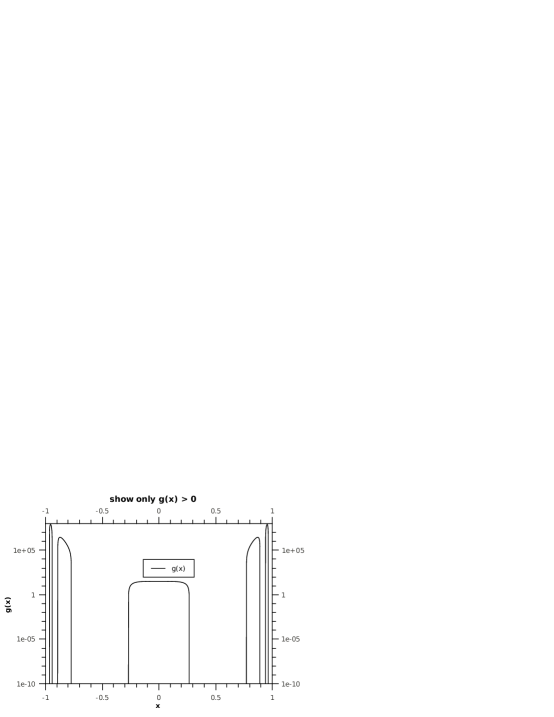
Figure 1: The figure of $g(x)$ in (90). The curve of $g(x)$ is plotted in semi-log scale only in the subintervals where $g(x)>0$. $g(x)=0$ for $x$ is outside of $(-1,1)$ has not been plotted for it is obvious that $g(x)=0$.

From (84), we see that the heat flux $f_{3}$ is changed by the term $\dfrac{\hbar^{2}}{24}\dfrac{\partial{{}^{3}V}}{\partial{x^{3}}}\rho_{0}$, which is the difference between the Boltzmann equation and the Wigner equation. The change of heat flux induces the change of the temperature (86) thus the electrons in part of the domain become cooler than the electrons in the else part of the domain. This makes the electrons with higher temperature moving to the domain with lower temperature (87), eventually resulting the redistribution of the density of the electrons (88). (89) shows that how the density $\rho$ changes at a very small $t$, and whether it will increase or decrease depends on the sign of $g(x)$, which is shown in Figure 1. So it is observed from Figure 1 that the particles will be redistributed because of the quantum term. Precisely, at a very small time $t$, the electron density in the subintervals of $(-1,1)$ where $g(x)>0$, whose curves are plotted in Figure 1, is increasing, and the electron density in the rest subintervals of $(-1,1)$ where $g(x)<0$ without its curves plotted, is decreasing.

In the remain part of this section, we present the 1D system obtained by truncating the expansion (61) at $M=4$, $5$ and $6$ for the reader’s convenience to carry out numerical simulations. If we truncate up to $M=4$, we obtain a closed system consisting of (68) - (70) and

$$\dfrac{\partial{f_{3}}}{\partial{t}}+4f_{3}\dfrac{\partial{u}}{\partial{x}}+\dfrac{1}{2}\mathcal{T}\rho\dfrac{\partial{\mathcal{T}}}{\partial{x}}+u\dfrac{\partial{f_{3}}}{\partial{x}}+4\dfrac{\partial{f_{4}}}{\partial{x}}=-\dfrac{f_{3}}{\tau}+\dfrac{\hbar^{2}}{24}\dfrac{\partial{{}^{3}V}}{\partial{x^{3}}}\rho,$$ (91)

and

$$\dfrac{\partial{f_{4}}}{\partial{t}}-\dfrac{f_{3}}{\rho}\dfrac{\partial{P}}{\partial{x}}+\mathcal{T}\dfrac{\partial{f_{3}}}{\partial{x}}+u\dfrac{\partial{f_{4}}}{\partial{x}}=-\dfrac{f_{4}}{\tau}.$$ (92)

And the system is collected into the matrix form (72) with $\boldsymbol{w}=\left(\rho,u,P/2,f_{3},f_{4}\right)^{T}$ and

$${\bf M}=\begin{pmatrix}u&p&0&0&0\\ 0&u&\dfrac{2}{\rho}&0&0\\ 0&3P&u&3&0\\ -\dfrac{P^{2}}{2\rho^{2}}&4f_{3}&\dfrac{P}{\rho}&u&4\\ 0&0&-\dfrac{f_{3}}{\rho}&\dfrac{P}{\rho}&u\end{pmatrix},$$ (93)

$${\bf G}=\begin{pmatrix}0&0&0&0&0\\ -\dfrac{\partial{V}}{\partial{x}}\dfrac{1}{\rho}&0&0&0&0\\ 0&0&0&0&0\\ \dfrac{\hbar^{2}}{24}\dfrac{\partial{{}^{3}V}}{\partial{x^{3}}}&0&0&-\dfrac{1}{\tau}&0\\ 0&0&0&0&-\dfrac{1}{\tau}\end{pmatrix}.$$ (94)

Similarly we can write out the system truncated at $M=5$ which consists of (68) - (70), (91) and

$$\dfrac{\partial{f_{4}}}{\partial{t}}-\dfrac{f_{3}}{\rho}\dfrac{\partial{P}}{\partial{x}}+5f_{4}\dfrac{\partial{u}}{\partial{x}}+\frac{5f_{3}}{2}\dfrac{\partial{\mathcal{T}}}{\partial{x}}+\mathcal{T}\dfrac{\partial{f_{3}}}{\partial{x}}+u\dfrac{\partial{f_{4}}}{\partial{x}}+5\dfrac{\partial{f_{5}}}{\partial{x}}=-\dfrac{f_{4}}{\tau},$$ (95)

and

$$\begin{split}&\dfrac{\partial{f_{5}}}{\partial{t}}-\dfrac{f_{4}}{\rho}\dfrac{\partial{P}}{\partial{x}}-\dfrac{3f_{3}}{\rho}\dfrac{\partial{f_{3}}}{\partial{x}}+\mathcal{T}\dfrac{\partial{f_{4}}}{\partial{x}}+u\dfrac{\partial{f_{5}}}{\partial{x}}=-\dfrac{f_{5}}{\tau}+\dfrac{\hbar^{4}}{1920}\dfrac{\partial{{}^{5}V}}{\partial{x^{5}}}f_{0},\end{split}$$ (96)

which is expressed into the matrix form (72) with where $\boldsymbol{w}=\left(\rho,u,P/2,f_{3},f_{4},f_{5}\right)^{T}$ and

$${\bf M}=\begin{pmatrix}u&p&0&0&0&0\\ 0&u&\dfrac{2}{\rho}&0&0&0\\ 0&3P&u&3&0&0\\ -\dfrac{P^{2}}{2\rho^{2}}&4f_{3}&\dfrac{P}{\rho}&u&4&0\\ -\dfrac{5Pf_{3}}{2\rho^{2}}&5f_{4}&\dfrac{3f_{3}}{\rho}&\dfrac{P}{\rho}&u&5\\ 0&0&-\dfrac{f_{4}}{\rho}&-\dfrac{3f_{3}}{\rho}&\dfrac{P}{\rho}&u\end{pmatrix},$$ (97)

$${\bf G}=\begin{pmatrix}0&0&0&0&0&0\\ -\dfrac{\partial{V}}{\partial{x}}\dfrac{1}{\rho}&0&0&0&0&0\\ 0&0&0&0&0&0\\ \dfrac{\hbar^{2}}{24}\dfrac{\partial{{}^{3}V}}{\partial{x^{3}}}&0&0&-\dfrac{1}{\tau}&0&0\\ 0&0&0&0&-\dfrac{1}{\tau}&0\\ -\dfrac{\hbar^{4}}{1920}\dfrac{\partial{{}^{5}V}}{\partial{x^{5}}}&0&0&0&0&-\dfrac{1}{\tau}\end{pmatrix}.$$ (98)

In the case of truncating at $M=6$, the moment system obtained consists of (68) - (70), (91), (95) and

$$\begin{split}\dfrac{\partial{f_{5}}}{\partial{t}}-\dfrac{f_{4}}{\rho}\dfrac{\partial{P}}{\partial{x}}&-\dfrac{3f_{3}}{\rho}\dfrac{\partial{f_{3}}}{\partial{x}}+6f_{5}\dfrac{\partial{u}}{\partial{x}}+3f_{4}\dfrac{\partial{\mathcal{T}}}{\partial{x}}\\ &+\mathcal{T}\dfrac{\partial{f_{4}}}{\partial{x}}+u\dfrac{\partial{f_{5}}}{\partial{x}}+6\dfrac{\partial{f_{6}}}{\partial{x}}=-\dfrac{f_{5}}{\tau}-\dfrac{\hbar^{4}}{1920}\dfrac{\partial{{}^{5}V}}{\partial{x^{5}}}f_{0},\end{split}$$ (99)

$$\begin{split}&\dfrac{\partial{f_{6}}}{\partial{t}}-\dfrac{f_{5}}{\rho}\dfrac{\partial{P}}{\partial{x}}-\dfrac{3f_{4}}{\rho}\dfrac{\partial{f_{3}}}{\partial{x}}+\dfrac{1}{2}\dfrac{\partial{\mathcal{T}}}{\partial{x}}\mathcal{T}f_{3}+\mathcal{T}\dfrac{\partial{f_{5}}}{\partial{x}}+u\dfrac{\partial{f_{6}}}{\partial{x}}=-\dfrac{f_{6}}{\tau}+\dfrac{\hbar^{2}}{24}\dfrac{\partial{{}^{3}V}}{\partial{x^{3}}}f_{3}.\end{split}$$ (100)

This system can be formulated in the matrix form of (72) with $\boldsymbol{w}=\left(\rho,u,P/2,f_{3},f_{4},f_{5},f_{6}\right)^{T}$ and

$${\bf M}=\begin{pmatrix}u&p&0&0&0&0&0\\ 0&u&\dfrac{2}{\rho}&0&0&0&0\\ 0&3P&u&3&0&0&0\\ -\dfrac{P^{2}}{2\rho^{2}}&4f_{3}&\dfrac{P}{\rho}&u&4&0&0\\ -\dfrac{5Pf_{3}}{2\rho^{2}}&5f_{4}&\dfrac{3f_{3}}{2\rho}&\dfrac{P}{\rho}&u&5&0\\ -\dfrac{3Pf_{4}}{\rho^{2}}&6f_{5}&\dfrac{2f_{4}}{\rho}&-\dfrac{3f_{3}}{\rho}&\dfrac{P}{\rho}&u&6\\ -\dfrac{P^{2}f_{3}}{2\rho^{3}}&0&\dfrac{Pf_{3}}{2\rho^{2}}-\dfrac{f_{5}}{\rho}&-\dfrac{3f_{4}}{\rho}&0&\dfrac{P}{\rho}&u\end{pmatrix},$$ (101)

$${\bf G}=\begin{pmatrix}0&0&0&0&0&0&0\\ -\dfrac{\partial{V}}{\partial{x}}\dfrac{1}{\rho}&0&0&0&0&0&0\\ 0&0&0&0&0&0&0\\ \dfrac{\hbar^{2}}{24}\dfrac{\partial{{}^{3}V}}{\partial{x^{3}}}&0&0&-\dfrac{1}{\tau}&0&0&0\\ 0&0&0&0&-\dfrac{1}{\tau}&0&0\\ -\dfrac{\hbar^{4}}{1920}\dfrac{\partial{{}^{5}V}}{\partial{x^{5}}}&0&0&0&0&-\dfrac{1}{\tau}&0\\ 0&0&0&\dfrac{\hbar^{2}}{24}\dfrac{\partial{{}^{3}V}}{\partial{x^{3}}}&0&0&-\dfrac{1}{\tau}\end{pmatrix}.$$ (102)

Observing M’s in (73), (93), (97), (101) and G’s in (74), (94), (98), (102), we find that the left hand side of the moment system of (72) is the exactly the same as the moment system derived from the classical Boltzmann equation, and the quantum mechanical terms with a typical characteristic which involves the high order derivatives of the potential $V$ are only appear in the matrices $G$ in the right-hand side of (72). It is clear that every $G$ is lower triangular. The formation of matrices $G$ shows that the quantum potential term works in the way by letting high-order moments get information from the moments of different lower orders, as low as to order $0$.

6 Conclusion

We extend the moment closure method [7] for the Boltzmann equation to its quantum counterpart, the Wigner equation. And we obtain a hyperbolic moment system, i.e., quantum hydrodynamic system. The method to derive the quantum hydrodynamic system with the global hyperbolicity is systematic that systems for arbitrary number of moments are obtained at once. Numerical simulations are to be carried out to demonstrate that the quantum effects are able to be captured by using the quantum hydrodynamic model derived.

References

• [1] M. Abramowitz and I. A. Stegun. Handbook of Mathematical Functions with Formulas, Graphs, and Mathematical Tables. Dover, New York, 1964.
• [2] J. D. Au, H. Struchtrup, and M. Torrilhon. $ET_{XX}$ — an equation generator for extended thermodynamics. Source available on request via M.Torrilhon@vt.tu-berlin.de.
• [3] J. D. Au, M. Torrilhon, and W. Weiss. The shock tube study in extended thermodynamics. Phys. Fluids, 13(8):2423–2432, 2001.
• [4] P. L. Bhatnagar, E. P. Gross, and M. Krook. A model for collision processes in gases. I. small amplitude processes in charged and neutral one-component systems. Phys. Rev., 94(3):511–525, 1954.
• [5] B. A. Biegel and J. D. Plummer. Comparison of self-consistency iteration options for the Wigner function method of quantum device simulation. Phys. Rev. B, 54:8070–8082, Sep 1996.
• [6] Z. Cai, Y. Fan, and R. Li. Globally hyperbolic regularization of Grad’s moment system in one dimensional space. Tech. Report, Institute of Math, Peking University, 2011-040, 2011.
• [7] Z. Cai, Y. Fan, and R. Li. Globally hyperbolic regularization of Grad’s moment system. Tech. Report, Institute of Math, Peking University, 2012-006, 2012.
• [8] Z. Cai and R. Li. Numerical regularized moment method of arbitrary order for Boltzmann-BGK equation. SIAM J. Sci. Comput., 32(5):2875–2907, 2010.
• [9] Z. Cai, R. Li, and Z. Qiao. NR$xx$ simulation of microflows with Shakhov model. SIAM J. Sci. Comput., 34(1):A339–A369, 2012.
• [10] Z. Cai, R. Li, and Y. Wang. Numerical regularized moment method for high Mach number flow. Commun. Comput. Phys., 11(5):1415–1438, 2012.
• [11] P. Degond, F. Méhats, and C. Ringofer. Quantum energy-transport and drift-diffusion models. J. Stat. Phys., 118:625–667, 2005.
• [12] P. Degond and C. Ringhofer. Quantum moment hydrodynamics and the entropy principle. Journal of Statistical Physics, 112:587–628, 2003.
• [13] ITWG editors. International Techonology Roadmap for Semiconductors. Technical report, Semiconductor Industry Association, http://www.itrs.net/Links/2009ITRS/, 2009.
• [14] D. K. Ferry and S. M. Goodnick. Transport in Nanostructures. Cambridge Univ. Press, Cambridge, U.K, 1997.
• [15] W.R. Frensley. Wigner function model of a resonant-tunneling semiconductor device. Phys. Rev. B, 36:1570–1580, 1987.
• [16] C. L. Gardner. The quantum hydrodynamic model for semiconductor devices. SIAM J. Appl. Math., 54:409–427, 1994.
• [17] A. Gehring and H. Kosina. Wigner function-based simulation of quantum transport in scaled DG-MOSFETs using a Monte Carlo method. J. Comput. Electr., 4:67–70, 2005.
• [18] H. Grad. On the kinetic theory of rarefied gases. Comm. Pure Appl. Math., 2(4):331–407, 1949.
• [19] H. Grad. The profile of a steady plane shock wave. Comm. Pure Appl. Math., 5(3):257–300, 1952.
• [20] M. Hillery, R.F. ÓConnell, M.O. Scully, and E.P. Wigner. Distribution functions in physics: Fundamentals. Physics Reports, 106(3):121–167, 1984.
• [21] X. Hu, S. Tang, and M. Leroux. Stationary and transient simulations for a one-dimensional resonant tunneling diode. Communications in Computational Physics, 4(5):1034–1050, 2008.
• [22] C. Jacoboni and P. Bordone. The Wigner-function approach to non-equilibrium electron transport. Rep. Prog. Phys., 67:1033–1071, 2004.
• [23] S. Jin and M. Slemrod. Regularization of the Burnett equations via relaxation. J. Stat. Phys, 103(5–6):1009–1033, 2001.
• [24] A. Jüngel. A note on current-voltage characteristics from the quantum hydrodynamic equations for semiconductors. Applied Mathematics Letters, 10(4):29–34, 1997.
• [25] N. Kluksdahl, A.M. Kriman, D.K. Ferry, and C. Ringhofer. Self-consistent study of the resonant tunneling diode. Phys. Rev. B., 39:7720–7735, 1989.
• [26] H. Kosina and M. Nedjalkov. Wigner function-based device modeling. In M. Rieth and W. Schommers, editors, Nanodevice Modeling and Nanoelectronics, volume 10 of Handbook of Theoretical and Computational Nanotechnology. American Scientific Publishers, 2006.
• [27] C. D. Levermore. Moment closure hierarchies for kinetic theories. J. Stat. Phys., 83(5–6):1021–1065, 1996.
• [28] P.L. Lions and T. Paul. Sur les mesure de Wigner. Rev. Mat. Ib., 9:553–618, 1993.
• [29] D. Querlioz, H.-N. Nguyen, J. Saint-Martin, A. Bournel, S. Galdin-Retailleau, and P. Dollfus. Wigner-Boltzmann Monte Carlo approach to nanodevice simulation: from quantum to semiclassical transport. J. Comput. Electron., 10:324–335, 2009.
• [30] X. Shan and X. He. Discretization of the velocity space in the solution of the Boltzmann equation. Phys. Rev. Lett., 80:65–68, Jan 1998.
• [31] S. Shao, T. Lu, and W. Cai. Adaptive conservative cell average spectral element methods for transient Wigner equation in quantum transport. Commun. Comput. Phys., 9:711–739, 2011.
• [32] H. Struchtrup. Stable transport equations for rarefied gases at high orders in the Knudsen number. Phys. Fluids, 16(11):3921–3934, 2004.
• [33] H. Struchtrup and M. Torrilhon. Regularization of Grad’s 13 moment equations: Derivation and linear analysis. Phys. Fluids, 15(9):2668–2680, 2003.
• [34] M. Torrilhon. Regularized 13-moment-equations. In M. S. Ivanov and A. K. Rebrov, editors, Rarefied Gas Dynamics: 25th International Symposium, 2006.
• [35] M. Torrilhon. Hyperbolic moment equations in kinetic gas theory based on multi-variate Pearson-IV-distributions. Commun. Comput. Phys., 7(4):639–673, 2010.
• [36] M. Torrilhon, J. D. Au, and H. Struchtrup. Explicit fluxes and productions for large systems of the moment method based on extended thermodynamics. Cont. Mech. and Ther., 15(1):97–111, 2002.
• [37] E. Wigner. On the quantum correction for thermodynamic equilibrium. Phys. Rev., 40(5):749–759, Jun 1932.
• [38] P.J. Zhao and D. Woolard. Wigner-poisson model based nano-electronic engineering modeling and design. Dynamics of continuous, discrete $\&$ impulsive systems, Series B, Applications $\&$ algorithms, 2:854–859, 2005.
• [39] J.-R. Zhou and D.K. Ferry. Simulation of ultra-small GaAs MESFET using quantum moment equations. IEEE Trans. Electron Devices, 39(3):473–478, 1992.